Adnan Kutay Yuksel![]() | Yilmaz Ar*
| Yilmaz Ar*![]()
© 2023 IIETA. This article is published by IIETA and is licensed under the CC BY 4.0 license (http://creativecommons.org/licenses/by/4.0/).
OPEN ACCESS
Today, all kinds of institutions and organizations depend on the Internet and information systems. They have been an inseparable part of human life. This brings out not only convenience, but also potentially devastating vulnerabilities. There are countless solutions for such risks and it is true that these solutions greatly contribute to security, but no effective solution has yet been found against Zero-Day malware. Zero-day malware is malicious software that has not yet been identified by competent authorities and is not classified as malicious software. A traditional malware detection tool can only detect previously detected software and classify it as malicious. Machine learning methods, which have proven effective in various domains, offer a promising approach to addressing Zero-Day malware. Throughout this study, a stable solution other than traditional methods have been investigated to overcome all kinds of malware. Instead of solutions consisting of complex, time-consuming and heterogeneous features (such as deleting/adding/changing files, monitoring registry records, or running processes) in various studies in the literature, a simple, low-time cost and stable solution with homogeneous features (only API calls) has been obtained. The 98.04% accuracy score shows that the method is quite successful. The importance of the study is having high accuracy using only API calls as features in malware detection. It has been realized that classical antivirus methods are no longer sufficient for combating malicious software.
cyber security, zero-day, malware detection, machine learning
Thanks to its many capabilities, the Internet has become a concept that not only people but also all kinds of institutions and organizations in the public and private sector depend on. With the dependence of all kinds of institutions and organizations (including governments, armies and civilian companies and institutions) on the internet infrastructure, data production speed and capacity have increased significantly. Technology dependency has expanded tremendously and is likely to increase exponentially in the years to come.
While cyber space has increased its impact, cyber attackers have intensified their efforts accordingly. Whether for ransom, insider threats, politics, competition, cyber warfare, anger, or any other reason, cyber attackers find different ways to damage, stop, alter or monitor systems and devices. These methods are mostly implemented through malicious software that causes ever-increasing prices. As time passes, cyber security and dealing with malware will always be of significant importance in information systems.
While some losses can be expressed in billions of dollars, even these levels are insufficient to express some types of loss. As disrupting education systems leads to cessation of education, destroying a forensic data base leads to injustice and freeing criminals, altering sanitary information contributes to inaccurate examinations and possibly deaths; by infiltrating the military systems of a superpower nation, results similar to those that could be achieved by an all-out war will be easily and directly achieved.
After all these disaster scenarios, there are things to overcome them. The first step to protecting systems and ensuring proper cyber security requires effective malware protection. Malware can vary in size from only a few KB to GBs, as well as differ in characteristics, type, function and target. Malware can disable your computer, monitor your keyboard and mouse movements and clicks. It can also steal your private and vital information such as IBAN number, bank card details, and personal secrets, use your actions as part of big data and even make your device a zombie or crypto-currency mining bot, resulting in illegal use. As you can see, malware can harm any person, system, organization or institution, including armies, governments, and intelligence agencies.
Along with the increase and diversification of potential dangers in cyber space, there are many developments in cyber damages studies. As malicious black hat hackers find new ways to break into systems and good white hat hackers try new ways to eliminate and reveal their covert actions, this war will forever continue. Additionally, malicious software is examined, and it is found that it is largely automated. This is done by examining and reproducing previously written malicious software in study [1].
Today, a developer who knows any programming language, including cyber security libraries, regardless of their knowledge of cyber security issues, can work on code available on many code repository sites such as GitHub, GitBucket, BitBucket, and Launchpad. Even if this code was previously included in the antivirus's database and was considered malware, it can generate new malware by changing the names of a few variables or functions. This tweaked software basically does the same job as the previous software. However, since its content has undergone minor changes to deceive antivirus systems, it will not be recognized by antivirus and will be treated as another piece of software. Thus, new malware can be produced without much effort. This is why a novel approach is needed to provide an efficient and automated way to deal with all these dangers. The greatest requirement of this system is not only to prevent it by making inferences based on the information given to it, but also to determine the patterns of operations performed on the devices and to comment on situations that have not been reported to it before as a result of these patterns.
The research contributes to the literature by providing a solution that enables the detection of malicious software universally. This is done by eliminating the weaknesses of conventional malware combat methods, which are still insufficient. The main idea behind the research will be explained later. By explaining what traditional methods are, why they are insufficient today, and by discussing what could be the most efficient way to deal with malware while maintaining simplicity and speed, a solution proposal will be presented.
In the field of cyber security, machine learning methods such as K-Nearest Neighbor (KNN), Naive Bayes Classifier, Decision Tree and Support Vector Machine (SVM) have proven to be indispensable tools in revealing malicious intentions of heterogeneous structures [2]. There were many studies that produced different solutions to detect and eliminate malware [3-7].
Traditional methods such as manual analysis, antivirus software are insufficient to deal with malware today. Because of information technologies, malware development has come a long way and malicious software numbers have increased tremendously. There are also more resources than ever before for software and malware development. Thus, anyone can easily find a malware sample on the Internet and modify it more or less to produce new malware that cannot be detected through antivirus software. In other words, antivirus tools keep the hash values of harmful files in their database. They determine whether the file is harmful by looking at whether the file's hash value is registered as malicious in the database. However, the file hash value can be changed without affecting the software. In theory, there can be an infinite number of software that does the same job.
The biggest challenges are using features that can only be verified in a single dataset or machine method, such as deleting, adding, and modifying (heterogeneous) files without any time/design/hardware/cost effectiveness, tracking registry records, and running processes.
It is clear that to detect whether software is malicious, a stable and robust solution should be developed. This solution does not depend on some basic rules and does not decrease its effectiveness from case to case. Machine learning approaches deliver what we expect. They adhere to the rules, but also capture malware behavior patterns.
Using features that consist of only API calls (homogeneous) and that can be verified in many logically different ways, not just in a dataset or machine method, ensuring time/design/hardware/cost effectiveness is actually our proposed solution.
Ijaz et al. [8] studied a different approach to analyze malware than usual methods. They employed not only dynamic analysis, but also static analysis. A malware analysis sandbox called “Cuckoo Sandbox” was utilized for dynamic analysis and more than 2300 features were extracted in this context. The PE-FILE program was used for static analysis and 92 features were extracted. For dynamic analysis, 4 types of features, namely Registry, DLLs, APIs and summary information were used. By using the combination of these 4 features, 9 different types of feature combinations were utilized. They also highlighted some of the features contributed most to the research as “significant features”. The research was conducted on a dataset consisting of a binary file of 49000 files, 39000 of which were labeled malware. The article underlines that neither static nor dynamic analysis alone analyzes a file. With this hybrid method, they achieved 97% accuracy while combining both.
Shijo and Salim [9] focused on the advantages of hybrid analysis methods consisting of both dynamic and static analysis. Both methods have their own pros and cons. They worked with their own dataset, where malware executables were collected from the VirusShare community website. For static analysis, PSI (Printable String Information) values were extracted as features, and “system call frequencies” were used to extract features for dynamic analysis. Instead of all the API calls in the dataset, API calls that took place more than twice were considered in feature determination. They also evaluated the use of n-grams and after doing some research they decided to use 3-API-call-grams and 4-API-call-grams. By making use of the Cuckoo Sandbox, three methods were applied: static method, dynamic method and hybrid method (consisting of both dynamic and static analyses). They achieved 95.8%, 97.1%, and 98.7% accuracy rates, respectively, and declared the hybrid method as the most accurate. The accuracy rates reported are 94.84%, 96.65% and 97.68% respectively.
Liu and Wang [10] used 21378 samples, including 13518 malicious and 7860 benign ones. They see the behavior of the software in virtual machines by running samples in the Cuckoo Sandbox for dynamic analysis. It also sets a threshold for sequences of 3 or more API calls. This means that if an API call is called 3 or more times, it is considered a feature. Interestingly, they did not use other behaviors such as registry, folders, etc. as used in our study. They partitioned the dataset into training, validation, and test set and constructed BLSTM as a detection model. In this study, in which “API calls” were considered as a feature, they obtained the most accurate score of 97.85% with the BLSTM method.
Sun et al. [11] produced their own dataset and method to transform sandbox logs into uniform, well-defined, shaped form. So they use a variety of features such as registry key changes, API calls, mutex operations, etc. As part of their system, they use some measures, such as converting all text to lowercase, using "/" as path delimiters, and removing "http" and "https" strings from website names. They also classified API calls into close_handle, reg_open, reg_create, reg_enumerate, reg_set, reg_query_key, reg_query, reg_del, open_file, create_file, copy_file, create_dir, and mutexes. They state that since they point to a novel method, they achieved accuracy rates between 74.87% and 100% in FFRI datasets of different years.
Choudhury et al. [12] do not contribute much to explain mutexes and their importance in malware analysis. They first explained the Cuckoo Sandbox and its implementation. They then highlighted the fact that nowadays malware authors bundle their code, which causes difficulties for malware analysts in static analysis. Later, mutexes, which are important signs of malicious software, were described as flags and programs that control simultaneous access to system resources. For this reason, it has been concluded that if more than one code sample is active in the system, only one sample will continue to run. In addition, malicious code may not achieve its purpose by stopping other software if more samples run at the same time.
Walker et al. [13] focused on an additional feature of the Cuckoo protected area, which is appreciated throughout the literature, and they focused the article on this feature. In the study, they discovered that the Cuckoo Sandbox was useful when analyzing malware samples, but the “threat scoring” feature was inefficient. After doing some research and working with their own malware samples from Malpedia, they point out that the “threat scoring” feature of the Cuckoo Sandbox needs to be improved. However, if we look at the information given on Cuckoo's official page and application interface in our own evaluation, the application developers already state that this feature is an emerging feature and they still continue to work for improvement. Therefore, labeling a test feature a threat is unfair to Cuckoo, the most advanced tool that possesses all of the characteristics and behavior of software.
Jamalpur et al. [14] explained techniques and environments. Firstly, Malwr (now called Cuckoo), JoeSandbox, ThreatExpert etc. They talked about common sandboxes like "m1.exe", which copied kernel132.dll files to kernel1.dll. Here, this expression is not “kernel” (letter k-letter e-letter r-letter n-letter e-letter l), but “kerne1” (letter k-letter e-letter r-letter n-letter e-number 1). It should not be overlooked that it is a scam. As a result, it takes more time to analyze malware samples as cyber-attacks increase day by day. It is concluded that using sandboxes like Cuckoo on virtual machines is the most efficient and safest solution for dealing with malware samples.
Irshad et al. [15] used the features extracted by the Genetic Algorithm in their article. Starting with some possible features, including API calls, Registry Keys, Windows Directories, Windows DLL file, EXE file of Windows system, exploiting the Genetic Algorithm, they have identified the 41 most valuable features. The study dataset consists of 236 samples, of which 121 are labeled as malware and 115 are labeled as non-malware. They state that they use three different classifiers. Finally, they state that they have 81.3% accuracy rates with the Support Vector Machine, 64.7% for the Naive Bayes classifier, and 86.8% for the Random Forest Classifier. While simpler and universal solutions are needed, as will be discussed in Section 3 later, it would not be wrong to admit that the accuracy rates they obtained by working on very heterogeneous features, as well as by genetic algorithms (which increase the time/hardware/information costs), are low.
Lengyel et al. [16] mainly described another dynamic malware analysis system called DRAKVUF in their study. By doing their work on the Xen Virtual Machine, they tried out novel methods such as execution monitoring, overcoming DKOM attacks, monitoring file system access with memory events, and handling files deleted from memory. Considering their effectiveness, they are very complex. They worked on some malware samples, including TDL4, Zeus, Shadowserver etc. Although they claim that DRAKVUF is an effective way to analyze malware samples, they do not give a scalable accuracy rate. Therefore, it is considered that there are many aspects to improve in the study and the article in which it was published.
Fujino et al. [17] utilized API calling topics to detect malware, which we found very useful. This is based on API calls, as we will do in this study. They began their work by noting that there were many API calls to deal with. A method was needed to figure out which one to select as a feature. Through their own logic, they calculated a threshold value experimentally. After working on API calls, if the API call value is below the specified threshold, it will be discarded. As a result, if it is above the threshold, it will be selected as a feature. In the article, they also stated that this threshold value between 0.1 and 0.5 would be the optimal approach. They continued their studies, which they continued as unsupervised, by stating that the studies they referred to in their articles also used supervised learning. However, since they failed to provide an accuracy rate, it is evident that the work they started was very good. However, it can be considered unfinished. As we will explain later in Section 4, it can be said that we have obtained a very high percentage of accuracy using API calls with a much simpler method.
Pirscoveanu et al. [18] used their own dataset of about 80000 samples downloaded from VirusShare. By running these samples in the sandbox (virtual machine) of the Cuckoo Sandbox, they also created a commonly employed whitelist of benign software. With this study, they aimed to eliminate unnecessary features. They use 4 types of information when dealing with malware: DNS information, files accessed, mutexes, and registry keys. They classify VirusTotal's tags into 4 main groups: Trojan, potentially unwanted program, adware, rootkit. At the end of their studies, they achieved an accuracy rate of 98% by implementing the tree-to-random forest algorithm.
Mehra and Pandey [19] focused on HCI (Human Computer Interaction), a very significant topic neglected in articles. This means that some malware works regardless of human interaction, but some require human interaction as a method of misleading. The article underlines that sandboxes are useful tools for analyzing malware. It says this is completely unacceptable for human-initiated malware. The article also compares some useful tools for malware analysis, various sandboxes for their effectiveness in dealing with event-triggered malware.
Udayakumar et al. [20] focused on reviewing the literature rather than revealing anything original in their work. Today, the study, which started with the importance of malware detection, continues with the need to focus on dynamic analysis instead of static analysis. More than 38 articles written in the field of malware detection/classification are evaluated. After the literature review described above, they provide basic information about malware analysis. The information is basically about “.exe” files and “.dll” files. Following the assessment that it may be beneficial to use safe “.dll” files to find malicious ones, “possibly malicious” and “possibly benign" “.dll” files are determined by comparing behaviors. The paper, which does not present a clear study, gives some recommendations for any application in this area towards the end. This can be accomplished using the Cuckoo Sandbox. As a result, as stated before, the article does not reveal a study or an accuracy rate, but consists of a literature review.
Many of these studies [16-21] provided their accuracy rates with the method they applied, but many of them either employed very limited datasets or did not share them. When comparing the work carried out in this study, no dataset was found other than the two datasets utilized throughout the study. These datasets are mentioned in Section 3. One study looked at the order in which API calls are executed, and the other study used the API call frequencies when similar API calls are grouped. Another one tried to consider failed, successful and total API call frequency counts and also one study considered the frequencies of API calls. However, they did not use benchmark datasets, instead they created and used their own datasets.
Therefore, there was not sufficient data for the final comparison made in Table 4 in Section 4. A dataset that did not provide accuracy rates in either dataset [22] could not be used. Only the accuracy values of the dataset's creators [23] could be compared. However, when making this comparison, the following points will be taken into account, which will reveal the importance of our work more clearly. First of all, the study does not use machine learning or deep learning methods. Compared to the accuracy percentages obtained by the study, it is clear that the 12-fold validation applied in our study will yield broader and more realistic results. Most importantly, the study first extracted malicious software from malware scanning and antivirus websites through these databases. Therefore, the accuracy rates achieved in our study (MDAPI), which is based only on Machine Learning without malware databases, are commendable.
3.1 Main idea behind the research
As was briefly discussed in Section 2, there is a lot of research into malware detection or classification. However, many use a wide range of features that complicate research and applications. In our view, a basic structure and faster implementation are needed. Most articles focus on the many different and complex features covered in Section 2. However, we consider “API calls” to be the feature that most clearly reveals what a software executes and how it behaves. From this perspective, we will have a basis for malware detection based on API calls extracted from dynamic malware analysis. Keeping the accuracy rate as high as possible while keeping simplicity and speed at the top will be the biggest defining feature of our study. This is malware detection with machine learning methods based on an application programming interface (MDAPI).
First, the "Characteristic API Call features" approach was adopted. This approach takes advantage of the fact that possible and common malware behaviors use similar API calls. Common malware behaviors and possible API calls for these behaviors are as follows:
• For keystroke registration: FindWindowsA, ShowWindow, GetAsyncKeyState, SetWindowsHookEx, RegisterHotKey, GetMessage, UnhookWindowsHookEx etc.
• For screen capture: GetDC, GetWindowDC, CreateCompatibleDC, CreateCompatibleBitmap, SelectObject, BitBlt, WriteFile etc.
• To avoid Anti-Debugging: IsDebuggerPresent, CheckRemoteDebuggerPresent, OutputDebugStringA, OutputDebugStringW etc.
• For Downloaders: URLDownloadToFile, WinExec, ShellExecute etc.
• For DLL Injection: OpenProcess, VirtualAllocEx, WriteProcessMemory, CreateRemoteThread etc.
• For Droppers: FindResource, LoadResource, SizeOfResource, LockResource etc.
• To change the Registry: RegCloseKey, RegOpenKeyExA, RegDeleteValueA etc.
The “Most Common API Calls" approach was adopted after reaching lower-than-expected accuracy rates with the “Characteristic API Call Features" approach. With this novel approach, it has been recognized that the most frequently used API calls can provide meaningful clues about any possibility of malware. These two approaches will be explained in more detail in the following sections.
3.2 Dataset
Throughout our study, API calls are preferred as potential features that the two datasets allow us, for the reasons explained in Section 3. First, the APIMDS (API-Based Malware Detection System) dataset, which was published in conjunction with the study [23] and is entirely based on API calls, is used. The size of the dataset is 112.7MB and it is a “.csv” file consisting of 23146 software samples. Of the samples, 14131 were “malicious”, 3137 were “benign", and 5878 were “unlabeled” (i.e., it is unknown whether they are malicious or benign). The number of instances columns is not specific, as different software uses different numbers of API calls.
To examine the dataset structure, the first column is a string that gives an idea of the software type. There are three possibilities regarding the string in the first column:
• If the string is empty, the software is “unlabeled”, meaning it is unknown whether it is malicious or benign.
• If the string contains the phrase “not-a-virus”, the software is labeled “benign”.
• Software is labeled “malware” if the string is not empty and does not contain “not-a-virus”.
Second, the dataset given in study [22] was used to compare our performance on the first dataset with a different dataset. The dataset, which is also available on Kaggle, consists of two different files with a total size of approximately 2.2GB. Both are “.txt” type files. The first file contains API calls and the second file contains malware types. In other words, the type of malware in the first file is written on the corresponding line number in the second file. This second dataset consists of 7107 malware samples. 832 of them are “Spyware”, 379 of them are “Adware”, and 891 of them are "Dropper". In this dataset, there are also “Downloader”, “Trojan”, “Worm”, “Virus”, and “Backdoor” types, each with 1001 instances. The number of sample columns is not specific, as different software uses different numbers of API calls, as in the first dataset. Since all samples are malware, our problem will be a classification problem, not a detection problem as in the first dataset.
Throughout the study, for convenience, the terms “first dataset”, which refers to the dataset published by Ki et al. [23], and “second dataset”, which refers to the dataset published by Catak et al. [22]. Table 1 shows the main structures of datasets.
Table 1. The datasets used in the study
|
No |
Dataset |
Task |
Number of Software |
Content |
|
1 |
APIMDS (API-Based Malware Detection System) dataset |
Classification |
23146 |
14131 Malicious, 3137 Benign, 5878 Unlabeled |
|
2 |
A comparison API Call dataset for Windows PE malware classification |
Detection |
7107 (all malicious) |
1001 Downloader, 1001 Trojan, 1001 Worm, 1001 Virus, 1001 Backdoor, 891 Dropper, 832 Spyware, 379 Adware |
The first dataset enabled binary detection, malicious or not. The column listed whether the software was malicious and the API calls it was running on. Since the second dataset lists the malware type column and the API calls that this malware runs on, we have used multi classification instead of binary detection, since all software is already malicious.
3.3 Preparation of dataset and feature extraction
For our purposes, some work needs to be done to get the first dataset ready for implementation in the first phase. Preparation and operations on an Ubuntu 18.04 LTS and 12GB RAM capable machine using Linux Bash scripts to process the data are as follows:
• Since data is presented in double-quoted strings, all starting and ending double quotes have been removed so that the data is clean strings to work on.
• Due to their indifference to the learning process, 17268 pieces of software, of which 14131 are malicious and 3137 benign were retained. In addition, 5878 unlabeled software was discarded.
• Two groups of API calls have been determined for the feature extraction phase. The first group is “API calls that occur in at least one malicious software but not in any benign software” (referred to as “Supposedly-Malicious API calls” in the rest of the study). The second group was “API calls that occurred in at least one benign software but were not involved in any malicious software” (which are to be referred to as Supposedly-Benign API calls in the rest of the study). But surprisingly, the first group, referred to as the Supposedly-Malicious group had 599 API calls, while the second group called the Supposedly-Benign group, had only 5 API calls. (The number of different API calls in the whole dataset is 1165). Considering the detailed study during the feature selection phase and the simplicity approach based on the research, 604 features (604=599 extracted from malware+4 extracted from benign software) were considered too many. In addition, it was evaluated that the selection of features only from malicious or only benign software would turn our machine learning-based work into a linear regression, and that this would be the result of a fixed algorithm, not machine learning, and as a result of these facts, other solutions were sought.
• As part of our search for a more suitable solution, we take a simpler approach. For this, it was thought to detect API calls dependent upon other API calls. The term “dependent” here means that an API call is included in the dataset only with another API call. This is not in instances where the other API call doesn’t happen. We thought we could simplify the features we extracted in this way. All API calls that have an impact on another API call have been detected. With this approach, the number of “Supposedly-Malicious API calls” was reduced from 599 to 387 and the number of “Supposedly-Benign API calls” from 5 to 4 (thus the total number of individual API calls was 391). However, the number 391 was considered too much for a simple and effective solution we needed.
• It is evaluated that some progress has been made, but there is still room for improvement. For “Supposedly-Malicious API calls” and “Unclear API calls” (API calls that cannot be grouped into the two previously mentioned groups-i.e., API calls that are involved in both at least one malware and at least one benign software), the most frequent number of occurrences should be considered. For “Supposedly-Benign API calls” nothing will be done since the number is 4 and it’s already low enough.
• “Supposedly-Malicious API calls” are listed in descending order of the number of occurrences in the software. API calls that occurred less than 85 (which is a heuristic criterion we determine based on the number of features we want to extract) in the entire dataset were finally identified as 44 “Supposedly-Malicious API calls”.
• “Uncertain API calls” are listed in descending order of the number of passes in the software examples. A total of 16 were determined for “Uncertain API calls”.
• Finally, the feature selection was completed with 44 Supposedly-Malicious, 4 Supposedly-Benign, and 16 Uncertain API calls, with a total of 64 features. In this way, a problem such as linearity mentioned in the previous articles was completely overcome. In this way, API calls (designed by us) were separated based on their characteristics and the most frequently used ones were selected, and steps were taken towards an effective and simple application.
• Considering the inequality of malicious and benign samples in the dataset, it was evaluated that the number of malicious samples (10994) should be equal to the number of benign samples (3137) to avoid an imbalance-bias problem. Although this will solve the imbalance-bias problem, it will cause the loss of more than half of the data in the dataset.
The accuracy rate obtained with 64 features selected as described above was 81.06%. When this success rate is examined in detail, it seems quite low compared to this detailed feature preparation process, which we can call the “Malicious/Benign Character API calls Approach”. Therefore, it was considered that another feature selection approach, which we can describe as the “Most Used API Calls Approach”, which deals with the number of API calls in the dataset, may be more useful. Accordingly, the number of API calls in the dataset was computed. All API calls were ranked in descending order of the total number of occurrences, which we consider their possible contribution to learning. And the numbers 10, 20, 40, 60, 80, 100, 200, 300, and 400 were chosen (intuitively) to see how much the first few "mostly occurring” API calls contributed to the accuracy rate. The accuracy rates, which we found insufficient in the “Malicious/Benign Character API Calls Approach”, increased significantly with the “Most Used API Calls Approach". When the simple feature extraction process was evaluated, it was more than satisfactory. Further evaluation, comparison and information on the “Most Used API Calls Approach" will be detailed in Section 4.
3.4 Representation of features
There are lots of researches that use API calls in various ways. Using API call frequencies [9, 17] using API call frequencies when similar API calls are grouped [11], using API calls executed in the first string of the software [18], the order in which API calls occur while running a software [5] and even the number of failures, successes and total API call frequency [8] studies have been conducted. However, our study will only deal with whether an API call is called and executed, keeping simplicity in mind.
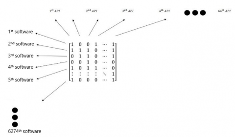
A notation called “Bag of Words” will be used to represent the selected features, which seem most appropriate to the situation. To create the structure in Figure 1 for this demonstration, the following preparations will need to be performed.
Let’s call the input matrix “A”. If xthsoftware contains yth feature (API call), then A[x][y]=1. If xth software does not contain yth feature (API call), then A[x][y]=0. All the 0 and 1 values given in Figure 1 are randomly chosen examples based on this explanation. If we interpret the shape based on what we have explained here, 1st software includes 1st API call (because A[0][0]=1), but does not include 2nd API call (because A[0][1]=0).
A[6274][64] is a matrix with 6274 rows (derived from the total software count of 3137 malicious and 3137 benign examples) and 64 columns (extracted from API calls, designated as 44 Supposedly-Malicious, 4 Supposedly-Benign and 16 Uncertain API calls).
We will have another matrix for the output, called “B”. If xth software is malicious, it will be expected to be B[x]=1, if xth software is benign, then B[x]=0. The B[6274][1] matrix consists of 6274 rows (derived from the total number of software (3137 malicious and 3137 benign samples) and only 1 column (derived from a single binary result, which will determine whether the software is malicious or not).
Figure 1. Implementation of the “Bag of Words” used in our study
3.5 Implementation
The input size of the artificial neural network derived from the feature size was chosen as 64 and then, 10, 20, 40, 60, 80, 100, 200, 300 and 400. The reasons will be explained in more detail in Section 4, as they were explained in the previous sections. Derived from the binary result (the closer to 0 the more likely it is to be benign and the closer to 1 the more likely it is to be malicious), the network output size is only 1. Intuitively, the number of layers according to the number of features was calculated as given in Table 2. The hidden layer size and the number of neurons were determined intuitively by considering the rule of thumb “two-thirds majority”, which determines the size of a layer, at the ratio of 2/3 of the size of previous layer.
In addition to the varying input, output, hidden layer size and number of parameters, there are some parameters that we consider to give optimal results in all the specified architectures. When detailing these, learning rate is 0.001. In order to overcome the saturation problem and the output value to be stable and logically oscillating between 0 and 1, sigmoid was chosen as the final activation function used in the last 336 (output) layer. All activation functions of all layers except the last layer are ReLU (Rectified Linear Unit).
The formulas of these two functions are given in Eq. (1), Eq. (2).
$\operatorname{Sigmoid}(x)=1 /\left(1+e^{-x}\right)$ (1)
$\operatorname{ReLU}(x)=\max (\mathbf{0}, \mathbf{x})$ (2)
Afterwards, an intuitive batch size adjusted to 12, 20, and 50 epochs is sufficient for the network to learn. However, 12 is the best value in the study. The values are optimized using “Binary Cross Entropy” and finally the results were verified by shuffling and using 12-fold cross validation to obtain more accurate results.
When the 100-75-50-30-20-12-8-1 architecture given in Table 2 is evaluated as an example, it will be seen that we have 6 hidden layers and that there are that many neurons in these layers, respectively. In addition, it should be noted that in the studies carried out, it was observed that the number of layers, like the number of features, increases accuracy to a certain extent. However, after a certain point, it causes more hardware and time costs than the contribution to success rates. It should be noted that the values with optimal results in the time-utility dilemma are presented above. The most accurate accuracy value obtained was 90.34%.
Table 2. Layer sizes representing neuron sizes from input (Left) to output (Right)
|
Number of Features |
Layer Sizes |
|
10 |
10-8-1 |
|
20 |
20-16-12-8-1 |
|
40 |
40-25-18-12-8-1 |
|
60 |
60-40-30-20-12-8-1 |
|
80 |
80-50-32-20-12-8-1 |
|
100 |
100-75-50-30-20-12-8-1 |
|
200 |
200-130-80-50-30-20-12-8-1 |
|
300 |
300-200-120-80-50-30-20-12-8-1 |
|
400 |
400-250-160-120-80-50-30-20-12-8-1 |
4.1 Results and comparison
As mentioned in previous sections, first the “Characterization” process with “Supposedly-Malicious” and “Supposedly-Benign” API calls is executed. After recognizing the drawbacks of this method, another approach was adopted to select features based on their occurrence in the entire dataset.
To be more specific, these processes can be summarized as follows:
• Approach to API Calls with Malicious/Benign Characteristics on First dataset: 64 Supposedly-characteristic API calls are used as features. The results obtained are not satisfactory.
• “Most Used API Calls” Approach in First dataset: The most used 10, 20, 40, 60, 80, 100, 200 and 400 API calls were selected as features, due to the lower than expected results with the “Malicious/Benign Characteristic API calls Approach”. The accuracy rate of the results is quite high.
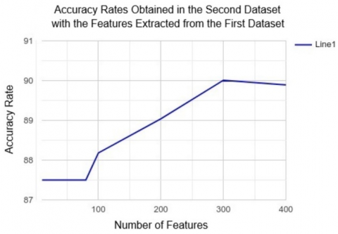
• Testing Features with Another dataset: After seeing the expected results with the "Most Used API calls Approach”, the same feature sets are tested as the features of the second dataset. The results are satisfactory as the features extracted from the first dataset identify patterns in another (second) dataset. Also, another challenge for this test is the nature of the second dataset, which allows classification only (the entire dataset consists of malware, contains no benign software, and contains malware classes in its labels), while the first dataset consists of both malicious and benign software, requiring detection, not classification. In this way, we have demonstrated that this approach is a very adaptable and universal solution for a wide range of tasks and datasets.
• Testing Approaches with Another dataset: Because satisfactory results were obtained in the previous stages, evaluating the approach instead of testing the features in another (second) dataset is utilized. In this context, the “Most Used API Calls Approach” has been tested on another (second) dataset. The most used API calls in the second dataset are extracted. The most used API calls 373 consisting of 10, 20, 40, 60, 80, 100, 200 and 278 are determined as the feature. It should be noted that while 300 and 400 features were tested in the first dataset, since the number of unique API calls in the second dataset is 278, 278 features were the only choice instead of 300 and 400 feature numbers. Although they are lower than in the first dataset, the results are still satisfactory. Obviously, this is due to the very small number of unique API calls (278) in the second dataset, and that on any dataset with sufficient unique API calls the results will be just as satisfactory as in the first dataset.
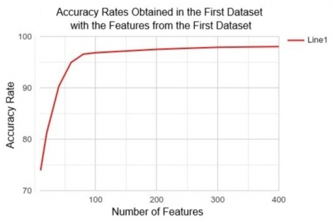
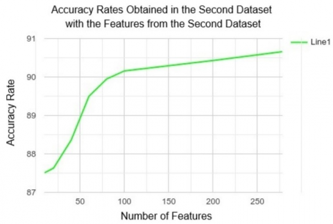
Figure 2, Figure 3 and Figure 4 show how feature counts contribute to accuracy rates based on our various approaches. Here, it is seen that as the number of features increases, success rates also increase (with decreasing acceleration). Therefore, if there is a need, the number of features can be determined using cost factors such as available time and equipment. The accuracy rates can be ignored to the desired degree, which also clearly demonstrates the system's flexibility.
In addition, based on the accuracy rates given in these figures, the fact that the study can be validated not only with the studied dataset but also with other datasets, and the success of the study on both detection and classification problems, should be accepted as an indication that it can bring a universal solution to the problem studied. In addition, it is clear that a very stable solution can be achieved above the accuracy rates obtained by increasing the variety and number of the dataset. This includes malicious and benign software types.
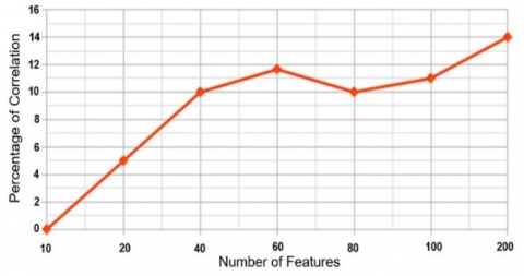
Another comparison was made as to whether a possible correlation could be established between the “Most Used API calls”, i.e., features of the two datasets. In the analysis, no significant correlation was found between the most frequently used API calls in the datasets. It is considered that this is due to the fact that the first dataset is suitable for detection solutions. It is composed of both malicious and benign samples. In contrast, the second dataset consists of only malicious samples and is appropriate for the classification problem. Both datasets consist of certain types of software and show different characteristics.
Figure 5 shows the correlation graph.
A variety of machine learning methods are used, and in Table 3, the accuracy values are displayed along with other metrics like precision, recall, and F1 values.
Figure 2. Accuracy rates obtained in the first dataset with the features extracted from the first dataset
Figure 3. Accuracy rates obtained in the second dataset with the features extracted from the second dataset
Figure 4. Accuracy rates obtained in the second dataset with the features extracted from the first dataset
Figure 5. Study of capturing possible correlation between features extracted from first and second datasets
The problems encountered in the literature review and comparison are detailed in Section 2. In addition, considering the issues mentioned in Section 2, the results obtained by this study are quite satisfactory, as can be seen in Table 4. The work mentioned in the first line here [23] is about signature-based detection, DNA sequence algorithms, etc., not machine learning/deep learning algorithms. It should be noted that they used a complex method consisting of studies. In other words, the working software first checks in antivirus databases. If it is already known as malware, the program labels it as malware and solves some of the problems with only signature-based algorithms. Therefore, the studies mentioned are very complex compared to our research and require more time. As a result (as in the first study), by comparing the signatures of the software (MD5, SHA-1, SHA-256, etc. hash values) with the databases of the malware, it does not benefit from previously detected malware, does not require handwritten algorithms, and uses machine learning/deep learning. It can easily be said that our research, which used learning methods, was very impressive.
Table 3. The results with respect to various metrics obtained by different methods
|
Metric |
Decision Tree |
K-Nearest Neighbour |
Naïve Bayes |
Random Forest |
Support Vector Machine |
Artificial Neural Network |
|
Accuracy |
89.29% |
90.01% |
59.00% |
89.77% |
90.09% |
98.04% |
|
Precision |
52.51% |
73.67% |
57.09% |
90.01% |
83.38% |
96.19% |
|
Recall |
89.09% |
65.07% |
87.30% |
97.51% |
55.83% |
98.74% |
|
F1 |
66.08% |
69.10% |
69.05% |
94.03% |
66.98% |
97.45% |
Table 4. Comparison of different accuracy values obtained by artificial neural network method with different approaches, datasets, feature number and selections (*Body of works including signature-based detection, genetic algorithm etc.)
|
Research that Gets the Score |
Dataset where Features were Extracted |
Approach Used |
Dataset where Results were Obtained |
Number of Features |
Problem Solved |
Obtained Accuracy |
|
[23] |
1st dataset |
Different Algorithms* |
1st dataset |
- |
Detection |
99.88% |
|
MDAPI |
1st dataset |
Malicious/Benign API Calls Approach |
1st dataset |
64 |
Detection |
81.06% |
|
MDAPI |
1st dataset |
Mostly-Used API Calls Approach |
1st dataset |
10 |
Detection |
73.89% |
|
MDAPI |
1st dataset |
Mostly-Used API Calls Approach |
1st dataset |
20 |
Detection |
81.19% |
|
MDAPI |
1st dataset |
Mostly-Used API Calls Approach |
1st dataset |
40 |
Detection |
90.34% |
|
MDAPI |
1st dataset |
Mostly-Used API Calls Approach |
1st dataset |
60 |
Detection |
94.96% |
|
MDAPI |
1st dataset |
Mostly-Used API Calls Approach |
1st dataset |
80 |
Detection |
96.57% |
|
MDAPI |
1st dataset |
Mostly-Used API Calls Approach |
1st dataset |
100 |
Detection |
96.84% |
|
MDAPI |
1st dataset |
Mostly-Used API Calls Approach |
1st dataset |
200 |
Detection |
97.50% |
|
MDAPI |
1st dataset |
Mostly-Used API Calls Approach |
1st dataset |
300 |
Detection |
97.91% |
|
MDAPI |
1st dataset |
Mostly-Used API Calls Approach |
1st dataset |
400 |
Detection |
98.04% |
|
MDAPI |
1st dataset |
Mostly-Used API Calls Approach |
2nd dataset |
10 |
Classification |
87.50% |
|
MDAPI |
1st dataset |
Mostly-Used API Calls Approach |
2nd dataset |
20 |
Classification |
87.50% |
|
MDAPI |
1st dataset |
Mostly-Used API Calls Approach |
2nd dataset |
40 |
Classification |
87.50% |
|
MDAPI |
1st dataset |
Mostly-Used API Calls Approach |
2nd dataset |
60 |
Classification |
87.50% |
|
MDAPI |
1st dataset |
Mostly-Used API Calls Approach |
2nd dataset |
80 |
Classification |
87.50% |
|
MDAPI |
1st dataset |
Mostly-Used API Calls Approach |
2nd dataset |
100 |
Classification |
88.18% |
|
MDAPI |
1st dataset |
Mostly-Used API Calls Approach |
2nd dataset |
200 |
Classification |
89.04% |
|
MDAPI |
1st dataset |
Mostly-Used API Calls Approach |
2nd dataset |
300 |
Classification |
90.01% |
|
MDAPI |
1st dataset |
Mostly-Used API Calls Approach |
2nd dataset |
400 |
Classification |
89.89% |
|
MDAPI |
2nd dataset |
Mostly-Used API Calls Approach |
2nd dataset |
10 |
Classification |
87.51% |
|
MDAPI |
2nd dataset |
Mostly-Used API Calls Approach |
2nd dataset |
20 |
Classification |
87.63% |
|
MDAPI |
2nd dataset |
Mostly-Used API Calls Approach |
2nd dataset |
40 |
Classification |
88.36% |
|
MDAPI |
2nd dataset |
Mostly-Used API Calls Approach |
2nd dataset |
60 |
Classification |
89.50% |
|
MDAPI |
2nd dataset |
Mostly-Used API Calls Approach |
2nd dataset |
80 |
Classification |
89.95% |
|
MDAPI |
2nd dataset |
Mostly-Used API Calls Approach |
2nd dataset |
100 |
Classification |
90.16% |
|
MDAPI |
2nd dataset |
Mostly-Used API Calls Approach |
2nd dataset |
200 |
Classification |
90.43% |
|
MDAPI |
2nd dataset |
Mostly-Used API Calls Approach |
2nd dataset |
278 |
Classification |
90.66% |
4.2 Discussion
For a more detailed and comprehensive discussion, there are specific implications and lessons to be drawn:
• Machine learning methods can detect and classify malware without complex algorithms or preparation processes.
• The number of features contributes to accuracy values. However, after a certain stage, with the increase in the number of features, the contribution decreases significantly compared to the time consumed. It is considered logical to increase the number of these features as much as possible and to an optimal degree (which can be considered 100-200 for this study) in a way that preserves the speed and simplicity of the algorithm, and then not to increase it in terms of time/hardware costs thus tuning all parameters optimally.
• It is seen that the first dataset has better accuracy rates than the second dataset. This is due to the large number of unique API calls in the initial dataset. That is, if we can have a sufficient number of correctly labeled malicious and benign software (and therefore unique API calls), it will be possible to create a “Machine Learning Antivirus”, producing a more universal solution to the malware detection problem.
It is possible to say that our research was successful in many respects. A number of obtained features are used within a logic that is completely homogeneous (consisting of only one type of feature-API calls) and without including any other feature types. We have achieved a higher level of success than many in the literature. These accuracy rates are also reasonable for multiple machine learning methods and different datasets.
A fast and robust solution has been developed with an emphasis on simpler and faster methods of malware detection using machine learning. Cyber security is a battle of wits and research should focus on more effective, faster and simpler methods.
After the work we have done in our research, it is no doubt that it will be much easier to create an antivirus framework using machine learning when there are numerous examples. This will put a heavy burden on malicious hackers (black hat hackers) and bring another perspective to a universal understanding of cyber security.
[1] Aliyev, V. (2010). Using honeypots to study skill level of attackers based on the exploited vulnerabilities in the network. Chalmers University of Technology.
[2] Kilgallon, S., De La Rosa, L., Cavazos, J. (2017). Improving the effectiveness and efficiency of dynamic malware analysis with machine learning. In 2017 Resilience Week (RWS). IEEE, pp. 30-36. https://doi.org/10.1109/RWEEK.2017.8088644
[3] Pascariu, C., Barbu, I.D. (2017). Dynamic analysis of malware using artificial neural networks: Applying machine learning to identify malicious behavior based on parent process hirarchy. In 2017 9th International Conference on Electronics, Computers and Artificial Intelligence (ECAI). IEEE, pp. 1-5. https://doi.org/10.1109/ECAI.2017.8166505
[4] Hansen, S.S., Larsen, T.M.T., Stevanovic, M., Pedersen, J.M. (2016). An approach for detection and family classification of malware based on behavioral analysis. In 2016 International Conference on Computing, Networking and Communications (ICNC). IEEE, pp. 1-5. https://doi.org/10.1109/ICCNC.2016.7440587
[5] Damodaran, A., Troia, F.D., Visaggio, C.A., Austin, T.H., Stamp, M. (2017). A comparison of static, dynamic, and hybrid analysis for malware detection. Journal of Computer Virology and Hacking Techniques, 13: 1-12. https://doi.org/10.1007/s11416-015-0261-z
[6] Darshan, S.S., Kumara, M.A., Jaidhar, C.D. (2016). Windows malware detection based on cuckoo sandbox generated report using machine learning algorithm. In 2016 11th International Conference on Industrial and Information Systems (ICIIS). IEEE, pp. 534-539. https://doi.org/10.1109/ICIINFS.2016.8262998
[7] Aslan, Ö., Samet, R. (2017). Investigation of possibilities to detect malware using existing tools. In 2017 IEEE/ACS 14th International Conference on Computer Systems and Applications (AICCSA), pp. 1277-1284. https://doi.org/10.1109/AICCSA.2017.24
[8] Ijaz, M., Durad, M.H., Ismail, M. (2019). Static and dynamic malware analysis using machine learning. In 2019 16th International Bhurban Conference on Applied Sciences and Technology (IBCAST). IEEE, pp. 687-691. https://doi.org/10.1109/IBCAST.2019.8667136
[9] Shijo, P.V., Salim, A.J.P.C.S. (2015). Integrated static and dynamic analysis for malware detection. Procedia Computer Science, 46: 804-811. https://doi.org/10.1016/j.procs.2015.02.149
[10] Liu, Y., Wang, Y. (2019). A robust malware detection system using deep learning on API calls. In 2019 IEEE 3rd Information Technology, Networking, Electronic and Automation Control Conference (ITNEC), pp. 1456-1460. https://doi.org/10.1109/ITNEC.2019.8728992
[11] Sun, B., Fujino, A., Mori, T., Ban, T., Takahashi, T., Inoue, D. (2018). Automatically generating malware analysis reports using sandbox logs. IEICE TRANSACTIONS on Information and Systems, 101(11): 2622-2632. https://doi.org/10.1587/transinf.2017ICP0011
[12] Choudhury, T., Jain, S., Aradhya, S.N., Kumar, P. (2018). An entire dynamic malware examination with near investigation of conduct examination sandboxes. In 2018 Second International Conference on Green Computing and Internet of Things (ICGCIoT). IEEE, pp. 583-590. https://doi.org/10.1109/ICGCIoT.2018.8752981
[13] Walker, A., Amjad, M.F., Sengupta, S. (2019). Cuckoo’s malware threat scoring and classification: Friend or foe? In 2019 IEEE 9th Annual Computing and Communication Workshop and Conference (CCWC), pp. 0678-0684. https://doi.org/10.1109/CCWC.2019.8666454
[14] Jamalpur, S., Navya, Y.S., Raja, P., Tagore, G., Rao, G.R.K. (2018). Dynamic malware analysis using cuckoo sandbox. In 2018 Second International Conference on Inventive Communication and Computational Technologies (ICICCT). IEEE, pp. 1056-1060. https://doi.org/10.1109/ICICCT.2018.8473346
[15] Irshad, A., Maurya, R., Dutta, M.K., Burget, R., Uher, V. (2019). Feature optimization for run time analysis of malware in windows operating system using machine learning approach. In 2019 42nd International Conference on Telecommunications and Signal Processing (TSP). IEEE, pp. 255-260. https://doi.org/10.1109/TSP.2019.8768808
[16] Lengyel, T.K., Maresca, S., Payne, B.D., Webster, G.D., Vogl, S., Kiayias, A. (2014). Scalability, fidelity and stealth in the drakvuf dynamic malware analysis system. In Proceedings of the 30th Annual Computer Security Applications Conference, pp. 386-395. https://doi.org/10.1145/2664243.2664252
[17] Fujino, A., Murakami, J., Mori, T. (2015). Discovering similar malware samples using API call topics. In 2015 12th Annual IEEE Consumer Communications and Networking Conference (CCNC), pp. 140-147. https://doi.org/10.1109/CCNC.2015.7157960
[18] Pirscoveanu, R.S., Hansen, S.S., Larsen, T.M., Stevanovic, M., Pedersen, J.M., Czech, A. (2015). Analysis of malware behavior: Type classification using machine learning. In 2015 International Conference on Cyber Situational Awareness, Data Analytics and Assessment (CyberSA). IEEE, pp. 1-7. https://doi.org/10.1109/CyberSA.2015.7166115
[19] Mehra, M., Pandey, D. (2015). Event triggered malware: A new challenge to sandboxing. In 2015 Annual IEEE India Conference (INDICON), pp. 1-6. https://doi.org/10.1109/INDICON.2015.7443327
[20] Udayakumar, N., Anandaselvi, S., Subbulakshmi, T. (2017). Dynamic malware analysis using machine learning algorithm. In 2017 International Conference on Intelligent Sustainable Systems (ICISS). IEEE, pp. 795-800. https://doi.org/10.1109/ISS1.2017.8389286
[21] Naeem, H., Alsirhani, A., Alshahrani, M.M., Alomari, A. (2022). Android device malware classification framework using multistep image feature extraction and multihead deep neural ensemble. Traitement du Signal, 39(3): 991-1003. https://doi.org/10.18280/ts.390326
[22] Catak, F.O., Yazı, A.F. (2019). A benchmark API call dataset for windows PE malware classification. arXiv Preprint arXiv: 1905.01999. https://doi.org/10.48550/arXiv.1905.01999
[23] Ki, Y., Kim, E., Kim, H.K. (2015). A novel approach to detect malware based on API call sequence analysis. International Journal of Distributed Sensor Networks, 11(6): 659101. https://doi.org/10.1155/2015/659101