Xingyu Ding![]() | Wenjun Hu*
| Wenjun Hu*![]() | Guanbing Hu
| Guanbing Hu![]() | Fang Liu
| Fang Liu![]()
© 2023 IIETA. This article is published by IIETA and is licensed under the CC BY 4.0 license (http://creativecommons.org/licenses/by/4.0/).
OPEN ACCESS
In the realm of geological and mineral exploration, remote sensing technology has emerged as a pivotal high-tech instrument. However, the effective interpretation of remote sensing images, especially in the context of heterogeneous data processing, noise, and the identification of fine granularity, remains a challenge. In this study, a novel method for the identification of mineral elements within remote sensing imagery was introduced. Firstly, a heterogeneous feature tensor migration technique anchored on the Coupled Heterogeneous Tucker Decomposition (CH-Tucker decomposition) was presented. Through this technique, multi-source remote sensing data were effectively processed and fused. Notably, associated data features from varying resolutions and angles were seamlessly coupled. Subsequently, an optical remote sensing image processing model founded on the RFDNet network was established. This model demonstrated robustness against noise data, thereby enabling the identification of mineral elements with a higher degree of granularity. The proposed methodology exhibited the capacity to extract mineral element information comprehensively and with remarkable accuracy. Thus, this research offers both valuable theoretical insights and practical evidence for furtherance in geological research and mineral element exploration.
remote sensing image processing, heterogeneous feature tensor migration, RFDNet network, mineral elements, fine granularity identification, noise suppression
In recent times, remote sensing technology has emerged as a cornerstone in geological exploration and mineral prospecting, proving itself instrumental in acquiring terrestrial surface information [1-4]. Images procured through remote sensing offer a wealth of geological information, enabling both macroscopic and microscopic viewpoints of mineral distribution. Such images are predominantly sourced from various remote sensing satellites and aircraft, encapsulating vast terrestrial expanses. Recognized for their consecutive, expansive coverage, and periodic nature, these images are pivotal for the identification of mineral elements [1-4].
However, with the incessant accumulation of remote sensing imagery data, researchers are now confronted with the formidable challenge of extracting precise and trustworthy mineral element details. The essence of this challenge lies in the need to interpret vast and intricate data, spanning various angles and scales, through automated and intelligent techniques [5]. In the domain of mineral element identification, data-driven methodologies associated with remote sensing image processing have been deemed invaluable. Such methodologies permit the extraction of multi-scale, multi-angle, and multi-source information, laying the foundation for deeper geological structure analyses, delineating ore belt distribution, and gauging mineral reserves [6-9]. The insights gleaned from these methods furnish pivotal details pertinent to the sustainable exploitation of mineral resources [6-9].
Yet, as remote sensing technologies and data acquisition instruments continue to evolve, there arises a surge in the volume and intricacy of remote sensing image data. Compounded by heightened heterogeneity and amplified noise interference, this escalation complicates data processing and the subsequent extraction of valuable information. Established methods, while somewhat effective, exhibit palpable shortcomings. For one, these traditional techniques often sidestep the inherent heterogeneity of multi-source data, culminating in fragmented and imprecise information extraction outcomes [10-14]. The multifaceted nature of such heterogeneity - spanning spatial, temporal, and spectral resolutions - necessitates more sophisticated processing strategies [15, 16]. Furthermore, the capabilities of current approaches in noise data management remain markedly limited. Their inability to pinpoint and mitigate interference compromises the reliability of mineral element identification results [17-19]. Finally, the increasing demands of processing vast swathes of remote sensing imagery data have accentuated challenges in achieving precise mineral element identification [20-22].
Addressing these imperatives, a novel method centered on remote sensing image processing was introduced. The primary segment of this research introduces a heterogeneous feature tensor migration technique anchored on the CH-Tucker decomposition. This method is adept at processing multi-source remote sensing data and adeptly fuses diverse resolution and angle-associated data features. Consequently, the accuracy and completeness of information extraction are enhanced. The secondary component outlines the construction of a fine granularity optical remote sensing image processing model, underpinned by the RFDNet network. This model's resilience to noise interference and its adeptness at mineral element identification suggest its potential to redefine standards in geological research and mineral exploration.
Remote sensing images, obtained from an array of sources, encompass a spectrum including optical remote sensing, radar remote sensing, and infrared remote sensing. These images, originating from diverse sources, exhibit variance in spatial, spectral, and temporal resolutions, leading to inherent data heterogeneity. An effective coupling of the associated features from these multi-source images is postulated to counteract this heterogeneity, potentially enhancing the precision and completeness of mineral element identification. It is further posited that these images, laden with rich geological information, may offer complementary insights when sourced differently. By effectively fusing associated features through coupling, a more comprehensive utilization of the information embedded within various remote sensing images is anticipated, thus potentially elevating the information retrieval efficacy concerning mineral elements.
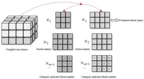
In the context of multi-source data, the varied resolutions and angles, derived from different satellites, are often represented by feature tensors of disparate sizes. Within this framework, a heterogeneous feature tensor migration technique, anchored on the CH-Tucker decomposition, was introduced in Figure 1. The foundational principle of this method revolves around the Tucker decomposition's capability to disintegrate input data into a core tensor coupled with a sequence of factor matrices. Here, the core tensor is leveraged as the low-dimensional representation of the initial data. Such a strategy is deemed effective in harnessing and extracting quintessential features from intricate high-dimensional datasets while simultaneously seeking latent shared representations within heterogeneous data. Consequently, the associated features from diverse data sources can be adeptly fused and extracted, paving the way for a more holistic and precise portrayal of mineral elements.
Figure 1. Schematic representation of CH-Tucker decomposition process
Assuming: $\left\{Z_a^u, t_a^u\right\}^{B a}{ }_{u=1}$ represents data of source 1; $\left\{Z_y^u, t_y^u\right\}^{B y}{ }_{u=1}$ represents data of source $2 ; Z^u{ }_a \in E^{U 1, U 2, \ldots, U M}$ and $t^u{ }_a \in$ $\{1, \ldots, L+1\}$ respectively represent samples coming from source 1 and their corresponding tags; $Z^u{ }_a \in E^{U 1, U 2, \ldots, U M}$ and $t^u{ }_a \in$ $\{1, \ldots, L\}$ respectively represent samples coming from source 2 and their corresponding tags. It is known that data $Z_a$ and $Z_y$ coming from the two sources can be represented by tensors of different dimensions, and they obey different marginal distribution $O\left(Z_a\right) \neq O\left(Z_y\right)$ and category conditional distribution $O\left(Z_a \mid t_a\right) \neq O\left(Z_y \mid t_y\right)$. So it's necessary to construct a mapping $v(\cdot)$ so that $O\left(v\left(Z_a\right) \mid t_a\right) \approx O\left(v\left(Z_y\right) \mid t_y\right)$. Considering that in semisupervised cases, $t_a$ and $t_y$ are unknown, then complete $P\left(\varphi\left(X_s\right) \mid y_s\right) \approx P\left(\varphi\left(X_t\right) \mid y_t\right)$ based on $t_a$ and $t_y$.
Assuming: $\left\{I_m^a \in E^{u m, U m}\right\}_{m=1}^M$ represents the multi-modal projection matrix of the search source domain, $\left\{I_m^y \in E^{u m, U m}\right\} M_{m=1}$ represents the multi-modal projection matrix of the target domain, $\left\{I_m^a \in E^{u m, U m}\right\}^M{ }_{m=1}$ and $\left\{I_m^y \in E^{u m, U m}\right\}^M{ }_{m=1}$ determine whether or not the heterogeneous feature tensors of remote sensing images of different resolutions and angles will be migrated to a common feature space. In this paper, the source domain samples were cascaded into an $M+m$ order tensor $Z_a=\left[Z^m a \ldots, Z^{B a} a\right]$, and the target domain samples were cascaded into an $\mathrm{M}+1$ order tensor $Z_y=\left[Z^m_y, \ldots, Z^{B y}_y\right]$. Referring to the Tucker decomposition, the low ranks of $Z_a$ and $Z_y$ were established as follows:
$Z_a \approx H_a \times{ }_1 I_1^a \times_2 \ldots \times_{M+1} I_{M+1}^a$ (1)
$Z_y \approx H_y \times_1 I_1^a \times_2 \ldots \times_{M+1} I_{M+1}^y$ (2)
Assuming: $H_a \in E^{u 1, \ldots, u M L}$ and $H_y \in E^{u 1, \ldots, u M, L}$ respectively represent the core tensor of source domain and the core tensor of target domain; the factor matrices satisfying the the orthogonality constraints $I^{a Y}{ }_m I^a{ }_m=U$, $1 \leq m \leq M$ and $I^{y Y}{ }_m I_m^y=U$, $1 \leq m \leq M$ are represented by $\left\{I^a_m\right\}^M{ }_{m=1}$ and $\left\{I^y_m\right\}^M{ }_{m=1}$ ; $I^a{ }_{M+1} \in E^{B a, L}$ and $I_{M+1}^y \in E^{B y, L}$ represent category indicator factor matrices; then, for an annotated remote sensing image sample $Z^u{ }_a\left(Z_a^u\right)$, if $t^u_a=k\left(t^u y=k\right)$, then let $I_M^a(u, k)=1$, and $I^a{ }_M(u, j)=0\left(I ^y_M(u, k)=1\right.$ and $I_M^y(u, j)=0$, wherein $j \neq k$; as for remote sensing image samples without any annotation, the category indicator factor matrices can be constructed as follows:
$\begin{aligned} & I_M^a(u,:) \geq 0 \sum_k I_M^a(u, k)=1 \quad \text { IF } \quad t_a^u=0 \\ & I_M^y(u,:) \geq 0 \sum_k I_M^y(u, k)=1 \quad \text { IF } \quad t_y^u=0\end{aligned}$ (3)
To get the effective factor matrix and core tensor of multi-source remote sensing images, an objective function was constructed as follows:
$\underset{H_a, H_y, I_m^a, I_m^y}{M \Pi N}\left\|Z_a-H_a \times_1 I_1^a \times_2 \ldots \times_{M+1} I_{M+1}^a\right\|_D^2+\left\|Z_y-H_y \times_1 I_1^y \times_2 \ldots \times_{M+1} I_{M+1}^y\right\|_D^2$ (4)
where, the dimension of the (M+1) mode Ha and Hy is L, so Ha and Hy can be decomposed into L sub-tensors; assuming Hla and Hly respectively represent the category centers of the source domain and the target domain, then the decomposed sub-tensors can be written as Ha = [H1a, ..., HLa] and Hy = [H1y, ..., HLy]. Assuming: $Q^a \in E^{B a, B y}$ represents the adaptive sample weight matrix of source domain; in this paper, based on Qa, outlier samples were automatically removed and embedded into the optimization; assuming γa represents a manually set constant used to determine the proportion of outlier samples, then there are:
$\underset{H_a, H_y, I_m^a, I_m^y, Q^a, Q^y}{M I N}\,\,\left\|Z_a \times_{M+1} Q^a-H_a \times_1 I_1^a \times_2 \ldots \times_{M+1} I_{M+1}^a \times_{M+1} Q^a\right\|_D^2+\left\|Z_y-H_a \times_1 I_1^y \times_2 \ldots \times_{M+1} I_{M+1}^y\right\|_D^2$$s.t. \sum_u Q^a(u, u)^2=\left(1-\lambda_a\right) B_a$$Q^a(u, k)=0 \forall u \neq k$$0 \leq Q^a(u, u)^2 \leq 1$ (5)
For the feature migration problem, it is required that the remote sensing image samples from different sources should have similar category conditional distributions, namely let H=Ha+Hy, then the objective function can be adjusted as follows:
$\underset{H, I_m^a, I_m^a, Q^a, Q^y}{M I N}\,\,\left\|Z_a \times_{M+1} Q^a-H_a \times_1 I_1^a \times_2 \ldots \times_{M+1} I_{M+1}^a \times_{M+1} Q^a\right\|_D^2+\left\|Z_y-H_a \times_1 I_1^y \times_2 \ldots \times_{M+1} I_{M+1}^y\right\|_D^2$ (6)
In order to improve the separability of the migration features of different-source remote sensing images, the difference between sub core tensors of different categories could be emphasized, that is, to maximize ∑l||Hl-1/LH×M+1rM||2D, wherein H = [H1, ..., HL] and rL = [1,1...1]L. Assuming: v represents regularization parameter, then the following formula gives the expression of the optimization problem of CH-Tucker decomposition:
$\begin{aligned} & \underset{H, I_m^a, I_m^y, Q^a, Q^y}{M I N}\,\,\left\|Z_a \times_{M+1} Q^a-H_a \times_1 I_1^a \times_2 \ldots \times_{M+1} I_{M+1}^a \times_{M+1} Q^a\right\|_D^2 \\ & +\left\|Z_y-H_a \times_1 I_1^y \times_2 \ldots \times_{M+1} I_{M+1}^y\right\|_D^2 \\ & -v \times\left(\sum_l\left\|H^l-\frac{1}{L} H \times_{M+1} r_L\right\|_D^2\right) \\ & \text { s.t. } \sum_u Q^a(u, u)^2=\left(1-\gamma_a\right) B_a \\ & Q^a(u, k)=0 \quad 0 \leq Q^a(u, u)^2 \leq 1 \leq \forall u \neq k \\ & I_{M+1}^s(u, k) \geq 0 \sum_k I_{M+1}^a(u, k)=1 I F \quad t_a^u=0 \\ & I_{M+1}^y(u, k) \geq 0 \sum_k I_{L+1}^y(u, k)=1 I F \quad t_y^u=0\end{aligned}$ (7)
After attaining the optimal factor matrix, the migration features of remote sensing images from different sources can be extracted through Tua=Zua×1IaY1×2...×MIaYM and Tuy=Zuy×1IyY1×2...×MIyYM.
In the realm of mineral element identification, the prominence of fine granularity classification tasks emerges due to the intricate compositions and diversity inherent to mineral elements. Notably, single-stage identification models often grapple with pitfalls, including ambiguities in classification outcomes and diminished classification scores. An associated challenge is observed wherein the quality of detection boxes is compromised by models filtering regression boxes based on classification efficacy. Such issues undermine the overall accuracy and completeness of the identification process, necessitating a model attuned to the demands of fine granularity tasks.
While two-stage identification models, utilizing the RPN structure, generate candidate boxes and subsequently determine RoIs, their merits in elevating recall rates and extracting quintessential target features are overshadowed by their reduced inference speed. Such impediments become particularly pronounced in scenarios demanding large-scale, real-time mineral element identification. A salient concern stems from the potential errors in fine granularity annotation data, often termed category noise. Owing to the marked similarities across categories, annotators confront challenges in distinctions, leading to misjudgments. Despite the presence of noise-laden training data, ensuring accurate learning of target representations for precise classification remains pivotal in mineral element identification. Regrettably, extant target detection algorithms display a lack of resilience to noise data. Thus, the pursuit of a neural network detection model adept at fine granularity classification, coupled with algorithmic efficiency, holds paramount significance to elevate identification precision, process noise data, and accommodate the intricacies of fine granularity tasks.
In light of these considerations, a single-stage fine granularity optical remote sensing image identification model, resilient to noise data, was introduced. Utilizing a single-stage anchor-based identification model as the foundational architecture ensures the model's basic performance metrics. Strategies were then employed to enhance the model's finesse in fine granularity classification. These included approaches to counteract the adverse impacts of noise annotation data on classification and initiatives to bolster the recall rate. Such refinements were demonstrated to effectively address prevalent challenges in fine granularity tasks, such as category confusion and suboptimal classification scores. Notably, an Anchor-Free approach was incorporated into the model, aiming to amplify the algorithm's computational velocity. This approach is poised to efficiently navigate fine granularity challenges, while simultaneously preserving the model's identification prowess.
3.1 Architecture of the RFDNet model for fine granularity identification
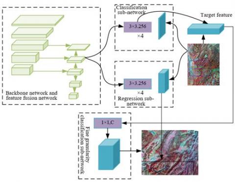
The constructed fine granularity identification model for mineral elements, denoted as RFDNet, boasts an intricate structure, encompassing a backbone network, a feature fusion network, a classification sub-network, a detection sub-network, and a fine granularity classification sub-network. Central to this architecture are the detection sub-network and the fine granularity classification sub-network (Refer to Figure 2).
Figure 2. Foundational framework of the RFDNet identification model
Responsibilities of the regression sub-network include the prediction of both the position and size of mineral elements within an image. An Anchor-Free approach is employed within the network, chosen for its ability to alleviate model complexity and computational demands. By directly forecasting the position and size of targets from feature images, without the reliance on preset anchors, the Anchor-Free method showcases its merit in parameter reduction and computational speed augmentation. Furthermore, it is posited that this approach bolsters the model’s adaptability towards targets of diverse dimensions and configurations. Defining m, y, e and n as distances from a sample point to the left, upper, right, and lower borders of the target HY box, and zv, tv as coordinates of the sample point, with zu, tu representing the coordinates of the target box vertices, the regression target manifests in an Anchor-Free format as:
$\left\{\begin{array}{l}m=z_v-M N N\left(z_u\right) \\ y=t_v-M I N\left(t_u\right) \\ e=M A X\left(z_u\right)-z_v \\ n=M A X\left(t_u\right)-t_v\end{array}\right.$ (8)
In the context of standardized coding, parameters m, y, e, and n undergo a transformation, rendering them as mb, yb, eb and nb, respectively, leading to the relationship:
$m_b=\frac{m}{S T}, y_b=\frac{y}{S T}, e_b=\frac{e}{S T}, n_b=\frac{n}{S T}$ (9)
The classification sub-network's primary function lies in discerning whether a given feature vector qualifies as a target, essentially demarcating between foreground and background. Given that this sub-network solely produces single-channel outcomes, inherent model complexities and computational loads experience significant reductions. This streamlined design allows for an efficient differentiation between the foreground and background, setting the stage for the ensuing fine granularity classification process.
The role of the fine granularity classification module emerges as extracting features predicated on the detection sub-network’s results, subsequently performing an in-depth granularity classification leveraging these features. Inspiration for this module’s design is drawn from the feature refinement methodologies characteristic of two-stage target detection models. Whilst ensuring the precision and discernibility of features, considerations towards algorithmic computational speed remain paramount. Equipped with this module, a more meticulous identification of mineral elements in images is achieved, culminating in the enhancement of mineral element identification accuracy.
3.2 Annotation assignment considerations in mineral element identification
In the endeavor of mineral element recognition through remote sensing images, a multitude of ores present nuanced distinctions in attributes such as shape, color, and texture. Such subtleties present significant challenges, especially when delving into fine granularity identification. Exacerbating this challenge are inherent characteristics of remote sensing images, where variability in acquisition equipment, shooting angle, meteorological conditions, and lighting conditions can introduce noise, complicating the annotation assignment task. More pertinently, the intricate and analogous nature of mineral features can, at times, lead to erroneous annotations or category noise.
In light of these complexities, a noise-robust annotation assignment strategy has been introduced. Utilizing both priori and posteriori position judgement criteria, this strategy has been observed to adeptly navigate potential annotation noise, thereby minimizing its detrimental impact on model training and recognition efficacy. The optimization involves computing and selecting the optimal joint Intersection over Union (IoU), leading to an enhanced precision in annotations tied to sample points. This, in turn, amplifies the mineral element identification accuracy. When juxtaposed with methods relying solely on posteriori criteria, this approach was seen to circumvent irrational annotation assignments in early training phases, hence expediting the model's convergence rate and enhancing training efficiency.
Within the RFDNet architecture, the criterion for noise-robust classification is determined by the loss emerging from the classification head's output, not the outcome of the fine granularity classification module. Such a design pivot shifts the classification benchmark from a nuanced granularity-based perspective to a more holistic, robust question of target presence.
Traditional annotation assignment approaches typically employ the loss function values of classification and regression as benchmarks for position and classification judgement. Upon these values, a cost matrix is constructed. Defining LOSSvma as the classification loss function, with ov and ovy representing classification predictions and the HY category respectively, and LOSSIoU symbolizing the IoU computation function, and where η1 and η2 denote the positional and classification judgement weights with γ being an additive term, the following relationship is deduced:
$\operatorname{COST}=\eta_1 \operatorname{LOSS}_{1 \text { vma }}\left(o^v, o_y^v\right)+\eta_2 \operatorname{LOSS}_{\text {IoU }}\left(o^n, o_y^n\right)+\gamma$ (10)
In mineral element identification via remote sensing images, it is commonly observed that the number of categories necessitating processing can be expansive. Given each prediction outcome and Ground Truth (GT), the conventional approach that utilizes the loss function of classification and regression for position and classification judgement demands a meticulous pre-assignment loss pair computation, followed by a subsequent loss calculation post-assignment. Such computational procedures are resource-intensive, and with a burgeoning category count, a consequential surge in computational overhead is inevitable, often culminating in a pronounced deceleration of training speed.
To navigate these computational intricacies, a strategy reminiscent of the AutoAssign method was introduced to construct the cost matrix. With the ability to directly compute the weighted sum of model outputs, thereby facilitating matrix construction, the AutoAssign-based approach showcased marked reductions in computational demands, subsequently fostering time efficiency in training. The final cost matrix is delineated as:
$\begin{aligned} & \operatorname{COST}=\eta_1 o^v+\eta_2 \operatorname{MAX}\left(\operatorname{IoU}\left(o^n, o_y^n\right), \operatorname{IoU}\left(A N, o_y^n\right)\right)+\gamma\end{aligned}$ (11)
The Centerness branch, as characterized in the FCOS, endeavors to predict each position's centrality, gravitating towards achieving elevated confidence at a target's central location. Yet, a few limitations of this method surface. Primarily, its foundation rests on an assumption that the center position of a target harbors the pinnacle of classification confidence. Such a presumption, however, might not consistently resonate with empirical observations, particularly when confronted with targets of irregular geometry or those exhibiting significant directional shifts. Secondly, the Centerness branch predominantly capitalizes on positional data, often sidelining potentially informative contextual cues, such as target size and texture. Such omissions could inadvertently compromise performance, especially in intricate scenarios. In such instances, the classification loss is articulated as:
$\operatorname{SSZ}(o)=-\left|o_y-o\right|^\alpha\left(\left(1-o_y\right) \log (1-o)+o_y \log (o)\right)$ (12)
where, t = {γ,γ, ..., IOI, ..., γ} and γ is defined as 1-IoU/B-1.
Contrastingly, the methodology that champions the Cost score, conceptualized as the harmonic mean of classification and positional criteria, manifests several merits. Foremost among these is the aptitude to judiciously harness both positional and classification data, striking a balance that augments detection and classification precision. Additionally, by eschewing assumptions regarding target morphology and location, it endows the model with enhanced adaptability to diverse target configurations and orientations. The amalgamation of position and classification criteria further enhances the model's prowess in managing noisy data, bolstering its resilience against erroneous annotations. For this methodology, t is represented as {γ, γ, ..., COST, ..., γ}, with γ delineated as 1-COST/B-1. The final loss function is thus:
$\operatorname{SSZ}(o)=-\operatorname{IoU}^\alpha\left(\eta_1 o+\eta_2 \operatorname{IoU}\right) \log (o)$ (13)
To elucidate the capabilities of the techniques presented, Figure 3 delineates the spectral reflectance curves for dolomite, specifically from the Dengying Formation of the Sinian System. Characterized primarily by its light grey thick-layered blocks of micrite dolomite, this lithological formation exhibits a greyish-white weathered surface. Observations have been noted on its light grey fresh surface, the presence of developed rock joints, and flat, smooth joint surfaces. An elevated degree of rock weathering is apparent.
For the purposes of a comparative study, data sources spanning four categories were employed: ZY1-02D AHSI and GF5 AHSI image data, spectral library data, and spectral morphology data garnered from field samples. Upon examination, it was observed that the spectral curves of dolomite acquired from field measurements exhibited high congruence with those from spectral libraries. Furthermore, spectral curves derived from optical satellites demonstrated consistency with those of ZY1-02D and GF5. Notably, these curves presented reflectance peaks at wavelengths of 2200nm and 2400nm, and absorption features around 2500nm, albeit with minor discrepancies in local positions.
Figure 3. Spectral reflectance curves of dolomite sourced from Dengying Formation of the Sinian System (as depicted from top left to bottom right: GF-5; ZY1-02D view; ZY1-02E; ZY1-02E 17810 view; field measurement; spectral library)
Figure 4. Field features of the aforementioned dolomite from the Dengying Formation of the Sinian System
Beyond the scope of Sinian dolomite, the study also cast its investigative lens on various rock minerals. The identifiability of each geological mass type was quantitatively assessed based on data collected in the field. Factors influencing this identifiability encompass the geological mass's dimensions, the employed image's scale, and the distinct shape and texture features of geological masses as portrayed in remote sensing images. An empirical approach for quantifying the identifiability of each geological mass type has been proposed, as illustrated in formulas presented in Figure 4.
Three primary categories of linear geological masses were identified: fracture structures, linear structures, and stratum bedding. Their respective lengths were recorded as 255m, 415m, and 345m. The scales at which these measurements were taken were determined to be 1:10,000 and 1:12,000, suggesting a unit length in the image represents either 10,000m or 12,000m on the actual ground.
Considering block geological masses, categories such as limestone interlayer, laminated basalt, and laminated limestone were examined. Their respective dimensions were recorded as 300×80m, 200×40m, and 360×35m, with scales of 1:12,000, 1:10,000, and 1:18,000 respectively. Closed-type geological masses, including dolomite, clastic rock strata, and surface coal seam outcrops, displayed diameters of 90m, 70m, and 60m, all captured at a scale of 1:8,000. Such detailed measurements are deemed essential for accurate interpretation of remote sensing images, facilitating precise identification and categorization of geological masses and thereby enhancing the accuracy of remote sensing analyses.
Within this dataset, it was observed that linear geological masses demonstrated high identifiability, with linear-shaped structures showcasing the most pronounced identifiability. Block geological masses presented medium-level identifiability, with laminated limestone emerging as the most identifiable. In contrast, closed-style geological masses exhibited lower identifiability, though dolomite was found to be relatively more identifiable within this category. It is noteworthy that this analysis predominantly focused on the size dimensions of geological masses. The potential impact of shape and texture features, evident in remote sensing images, on the identifiability of these geological masses remains unexplored and warrants further investigation.
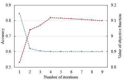
Figure 5. Curves showcasing identification accuracy and the value of the objective function across varying iteration numbers
An examination of Figure 5 reveals the model's identification accuracy and objective function value during training iterations. The peak accuracy, amounting to 0.845, was attained during the first iteration. Subsequently, a decline in accuracy was observed, stabilizing at approximately 0.6 between iterations 4 and 9. Concurrently, the objective function's value displayed an ascending trend, initiating from 8.83 and plateauing around 9.1. Such a trajectory suggests a rapid initial feature-learning phase by the model, leading to high accuracy. However, subsequent iterations seemingly induced over-fitting to the training data, reflected in the decreased accuracy. The stabilization of the objective function value signifies the model's convergence during the iterations, indicating a satisfactory fitting degree.
In Figure 6, the performance of the Tucker decomposition model under varying annotated sample proportions and regularization parameters is depicted. A significant influence of these parameters on model performance was noted. As illustrated, a general increase in the proportion of annotated samples corresponded to an enhancement in model accuracy in most instances. Such an improvement can be attributed to the availability of augmented data for model training, thereby bolstering the model's predictive capabilities. Distinct patterns were observed when evaluating the effect of different regularization parameters. For parameters set at 0.5 and 1, a synchronous increase in accuracy with annotated sample proportion was witnessed. Conversely, for values of 1.5 and 2, the fluctuation in accuracy across varying annotated sample proportions remained relatively inconspicuous. An elevation in the regularization parameter seemingly simplified the model, reducing potential overfitting. While this curtailed overfitting to an extent, it also might have inhibited the model's capacity to decipher intricate data patterns. The apt selection of both annotated sample proportion and regularization parameters, therefore, emerges as crucial for the efficacy of the proposed method, the optimal configuration of which may vary contingent on specific datasets and tasks.
Figure 6. Accuracy trends of CH-Tucker decomposition under varied annotated sample proportions
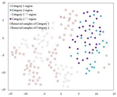
Figure 7. Visualization of migration features in remote sensing images across source and target domains
In this research, Tucker decomposition was utilized to extract migration features from remote sensing images. A weighted factor matrix was employed, effectively mitigating the influence of outliers, leading to the extraction of migration features of notable distinguishability. To empirically demonstrate this advantage, an experiment was conducted on an appropriate dataset. Three outlier samples, possessing azimuth angles ranging between 90 and 135 degrees, were incorporated into the source domain samples to serve as potential disruptions. With the Tucker decomposition parameter calibrated to 0.1, visual representations, both pre- and post-feature extraction, were generated via the t-SNE method. A detailed analysis of these visual outcomes can be discerned in Figure 7. It was postulated that the sample distribution within the source domain might undergo alterations subsequent to the inclusion of outlier interference. Nevertheless, the migration features, as isolated by the Tucker decomposition, are conjectured to neutralize this external perturbation to a degree. This implies that the source domain's feature distribution could align more congruently with that of the target domain, which, within the visual results, could manifest as an enhanced proximity between the distributions of source and target domain samples in a 2D space.
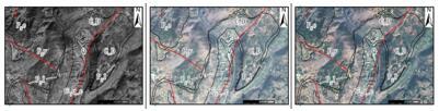
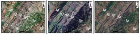
Figures 8-11 furnish a comparative examination of remote sensing geological element identification predicated upon data from panchromatic images, multi-spectral images, and fused images captured by optical satellites. Preliminary observations unveiled that the panchromatic and multi-spectral images offered limited distinguishability of geological masses, a constraint predominantly imposed by the images' scale and grey scale nuances. Moreover, the multi-spectral images exhibited blurring and mosaic patterns. In stark contrast, fused images manifested pronounced color tone variances between geological masses, indicative of enhanced distinguishability.
Figure 8. Comparative visualization of the 1:100000 mapping effect for remote sensing geological element identification - Panchromatic image (left), Multi-spectral image (middle), Fused data image (right)
Figure 9. Comparative visualization of the 1:100000 mapping effect for remote sensing geological element identification across different remote sensing data types - S2A (left), SPOT6 fusion (middle), GJ-1 fusion (right)
Figure 10. Comparative visualization of the 1:50000 mapping effect for remote sensing geological element identification - Panchromatic image (left), Multi-spectral image (middle), Fused data image (right)
Figure 11. Comparative visualization of the 1:50000 mapping effect for remote sensing geological element identification across different remote sensing data types - S2A (left), SPOT6 fusion (middle), GJ-1 fusion (right)
In the realm of remote sensing identification of geological elements, traditional methodologies, particularly those employing panchromatic and multi-spectral techniques, were found to be potentially inadequate in accurately discerning all geological elements, especially at finer scales. However, the incorporation of a feature fusion approach, leveraging multi-source remote sensing images, was observed to augment the distinguishability significantly.
The method of fine granularity identification introduced in this research demonstrated marked benefits. Primarily, a heightened ability was noted in capturing intricate details of geological masses, thus amplifying their distinguishability through refined granularity processing of the remote sensing images. Secondly, by adopting a noise-robust annotation assignment strategy, disturbances inherent in the images and potential instability were effectively mitigated, culminating in an enhancement in identification precision. Furthermore, the utilization of a cost matrix construction strategy, reminiscent of the AutoAssign approach, was revealed to considerably curtail computational burdens and expedite the training phase. Consequently, it can be inferred that the fine granularity identification method elucidated in this investigation can yield superior outcomes in the domain of geological element identification within remote sensing imagery.
In the pursuit of advancing fine granularity identification of geological elements using remote sensing images, challenges associated with intricate noise and the diversity of categories within these images were addressed. A novel approach was introduced in this study, utilizing CH-Tucker decomposition, which seamlessly integrated both a noise-robust annotation assignment strategy and a method akin to AutoAssign for cost matrix construction. This approach aimed to enhance the efficiency in processing and improve the accuracy of identification within remote sensing images.
Upon evaluation, it was observed that the delineated method exhibited both a notable accuracy and robustness when tasked with processing multi-source remote sensing image data. Particularly, as the number of iterations augmented, the accuracy was maintained, while a decline was noted in the value of the objective function, suggesting superior convergence performance. Furthermore, this approach was discerned to uphold its accuracy irrespective of variations in the proportion of annotated samples or changes in the regularization parameter, emphasizing its versatility in adapting to varying conditions of annotated samples and regularization intensities.
Synthesizing the findings and evaluations, it can be inferred that the method introduced, focusing on fine granularity identification of geological elements via CH-Tucker decomposition, possesses commendable noise resilience, swift training capabilities, and exemplary identification performance. Consequently, its potential applications in the broader realm of remote sensing geological element identification are vast, and its contribution to the academic discourse is deemed substantial.
This paper was supported by Hunan Provincial Natural Science Foundation of China (Grant No.: 2023JJ50339) and the Natural Science Foundation of Hunan Province, China (Grant No.: 2023JJ30212).
[1] Zheng, Z. (2023). Research on the application of remote sensing and GIS technology in railroad engineering geology survey. In Third International Conference on Sensors and Information Technology (ICSI 2023), Xiamen, China, pp. 74-79. https://doi.org/10.1117/12.2679143
[2] Bi, X., Jiang, L., Dong, Q., Wang, D. (2022). Hyperspectral remote sensing image processing and information extraction technology research in geological recognition application. In 2022 IEEE Asia-Pacific Conference on Image Processing, Electronics and Computers (IPEC), Dalian, China, pp. 936-938. https://doi.org/10.1109/IPEC54454.2022.9777528
[3] Oldenborger, G.A., Short, N., LeBlanc, A.M. (2022). Permafrost thaw sensitivity prediction using surficial geology, topography, and remote-sensing imagery: a data-driven neural network approach. Canadian Journal of Earth Sciences, 59(11): 897-913. https://doi.org/10.1139/cjes-2021-0117
[4] Sun, S., Dustdar, S., Ranjan, R., Morgan, G., Dong, Y., Wang, L. (2022). Remote sensing image interpretation with semantic graph-based methods: A survey. IEEE Journal of Selected Topics in Applied Earth Observations and Remote Sensing, 15: 4544-4558. https://doi.org/10.1109/JSTARS.2022.3176612
[5] Chandra, N., Vaidya, H. (2022). Human cognition based models for natural and remote sensing image analysis. In International Conference on Machine Intelligence and Signal Processing, pp. 617-628. https://doi.org/10.1007/978-981-99-0047-3_52
[6] Peyghambari, S., Zhang, Y. (2021). Hyperspectral remote sensing in lithological mapping, mineral exploration, and environmental geology: an updated review. Journal of Applied Remote Sensing, 15(3): 031501. https://doi.org/10.1117/1.JRS.15.031501
[7] Mu, F., Li, J., Shen, N., Huang, S., Pan, Y., Xu, T. (2022). Pixel-Adaptive Field-of-View for remote sensing image segmentation. IEEE Geoscience and Remote Sensing Letters, 19: 1-5. https://doi.org/10.1109/LGRS.2022.3187049
[8] Ding, H., Jing, L., Xi, M., Bai, S., Yao, C., Li, L. (2023). Research on scale improvement of geochemical exploration based on remote sensing image fusion. Remote Sensing, 15(8): 1993. https://doi.org/10.3390/rs15081993
[9] Torres Gil, L.K., Valdelamar Martínez, D., Saba, M. (2023). The widespread use of remote sensing in asbestos, vegetation, oil and gas, and geology applications. Atmosphere, 14(1): 172. https://doi.org/10.3390/atmos14010172
[10] Xi, J., Ersoy, O. K., Cong, M., Zhao, C., Qu, W., Wu, T. (2022). Wide and deep fourier neural network for hyperspectral remote sensing image classification. Remote Sensing, 14(12): 2931. https://doi.org/10.3390/rs14122931
[11] Ma, J., Lu, D., Shi, G., Li, Y. (2022). Remote sensing image change detection based on attention and convolutional neural network. In Proceedings of the 3rd International Conference on Geology, Mapping and Remote Sensing, Zhoushan, China, pp. 588-593. https://doi.org/10.1109/ICGMRS55602.2022.9849260
[12] 14. Yao, M., Huang, J., Zhang, M., Zhou, H., Kuang, L., Ye, F. (2022). A comprehensive evaluation method for topographic correction model of remote sensing image based on entropy weight method. Open Geosciences, 14(1): 354-366. https://doi.org/10.1515/geo-2022-0359
[13] Sun, Z., Li, P., Meng, Q., Sun, Y., Bi, Y. (2023). An Improved YOLOv5 method to detect tailings ponds from high-resolution remote sensing images. Remote Sensing, 15(7): 1796. https://doi.org/10.3390/rs15071796
[14] Xu, Y. (2021). Application of remote sensing image data scene generation method in smart city. Complexity, 2021: 6653841. https://doi.org/10.1155/2021/6653841
[15] Zheng, Z., Yang, C., Zhao, J., Feng, Y. (2022). Remote sensing geological classification of sea islands and reefs based on Deeplabv3+. In 2022 7th International Conference on Intelligent Computing and Signal Processing (ICSP), Xi'an, China, pp. 1907-1910. https://doi.org/10.1109/ICSP54964.2022.9778709
[16] Pan, T., Zuo, R., Wang, Z. (2023). Geological mapping via convolutional neural network based on remote sensing and geochemical survey data in vegetation coverage areas. IEEE Journal of Selected Topics in Applied Earth Observations and Remote Sensing, 16: 3485-3494. https://doi.org/10.1109/JSTARS.2023.3260584
[17] Li, H., Yang, W. (2021). Application of high-resolution remote sensing image for individual tree identification of pinus sylvestris and pinus tabulaeformis. Wireless Communications and Mobile Computing, 2021: 7672762. https://doi.org/10.1155/2021/7672762
[18] Zhao, X., Zhang, J., Tian, J., Zhuo, L., Zhang, J. (2020). Residual dense network based on channel-spatial attention for the scene classification of a high-resolution remote sensing image. Remote Sensing, 12(11): 1887. https://doi.org/10.3390/rs12111887
[19] Xun, Z., Zhao, C., Kang, Y., Liu, X., Liu, Y., Du, C. (2022). Automatic extraction of potential landslides by integrating an optical remote sensing image with an InSAR-Derived deformation map. Remote Sensing, 14(11): 2669. https://doi.org/10.3390/rs14112669
[20] Bishta, A.Z., Qudsi, E.Z. (2023). Implementation of space imageries, remote sensing and GIS techniques in the geological and geomorphological analysis of Wadi Fatima drainage basin, Saudi Arabia. Egyptian Journal of Remote Sensing and Space Science, 26(3): 563-579. https://doi.org/10.1016/j.ejrs.2023.06.006
[21] Yan, D., Zhang, H., Li, G., Li, X., Lei, H., Lu, K., Zhang, L., Zhu, F. (2022). Improved method to detect the tailings ponds from multispectral remote sensing images based on faster R-CNN and transfer learning. Remote Sensing, 14(1): 103. https://doi.org/10.3390/rs14010103
[22] Chen, N., Zhang, B. (2022). Multi-scale semi-coupled convolutional sparse coding for the super-resolution reconstruction of remote sensing image. Journal of Computer-Aided Design and Computer Graphics, 34(3): 382-391.