Sunitha Munappa![]() | J. Subhashini*
| J. Subhashini*![]() | Pallikonda Sarah Suhasini
| Pallikonda Sarah Suhasini![]()
© 2023 IIETA. This article is published by IIETA and is licensed under the CC BY 4.0 license (http://creativecommons.org/licenses/by/4.0/).
OPEN ACCESS
Accurate metastasis prediction in breast cancer (BC) patients is crucial for timely treatment, thereby reducing life-threatening risks. Traditional methods involve manual observation of whole slide images (WSIs) to identify tumor cells, necessitating extensive expertise and resulting in a time-consuming process. Recently, deep learning techniques have been employed for precise tumor cell detection. However, automatic detection methods face challenges such as limited availability of large datasets and the ambiguity between cancer cell structures and normal tissue. This paper proposes a novel deep stacked ensemble architecture to address these challenges. The proposed model incorporates three pre-trained models, namely RESNET50, EfficientNet B3, and DenseNet121, with single, double, and triple fully connected layers for each architecture, yielding nine models. Among these, three heterogeneous models were selected for the stacking ensemble. The performance of these models and the deep stacked ensemble was investigated and compared using the CAMELYON 17 challenge dataset, which contains lymph node WSIs of BC patients. Results demonstrate that the deep stacked ensemble outperforms individual models. In this prediction task, recall is more critical than precision; thus, the trade-off between recall and precision was also examined.
metastasis, Whole Slide Image (WSI), deep learning architectures, ensemble, stacking
Breast cancer (BC) metastasis is a primary cause of increased mortality rates among BC patients [1]. Early detection of BC is vital for prolonging patient survival, but identifying breast tumors at the initial stage can be a challenging task. Many women do not undergo regular mammogram check-ups, and palpation may only detect tumors after significant growth [1]. Consequently, most BC patients are diagnosed beyond the initial stage. Metastasis refers to the recurrence of cancer, where secondary tumors form from the primary tumor, spreading cancer cells to other body parts such as the brain, liver, bone, and lungs [2]. Accurate prediction of metastasis occurrence can facilitate proper medication and ultimately extend patient lifespan. By analyzing tumor cells in lymph nodes, metastasis prediction becomes possible. Small lymph node samples are typically examined for tumor cells on whole slide images (WSIs) through a microscope. However, feature extraction for classification presents numerous challenges, particularly due to the similarities between cancer cell structures and normal tissue. Conventional feature extraction methods are generally unsuitable for metastasis recognition. Recently, convolutional neural networks (CNNs) have demonstrated their ability to automatically extract features for various image recognition tasks [3], including cancer cell recognition. In this study, we propose a deep learning (DL) approach using CNNs for the automatic feature extraction of cancer cells. Our contributions are as follows:
This paper is organized as follows: Section 2 presents preliminaries, Section 3 reviews the relevant literature, Section 4 introduces the proposed deep stacked ensemble and discusses the diversity measure and systematic approach, Section 5 describes the dataset and methodology, Section 6 presents results and analysis, Section 7 compares the performance of the proposed architecture and base classifiers, and Section 8 concludes the paper.
In this section, we introduce the basic concepts of learning methods relevant to our study.
2.1 Deep Learning (DL)
DL is a subset of machine learning that involves neural networks with hundreds of deep layers and numerous parameters. When trained with large datasets, DL networks can significantly improve performance. CNNs [4] are particularly suitable for image classification applications.
2.2 Ensemble
Ensemble learning is a machine learning technique that enhances model metrics by combining the results of two or more models [5]. In this study, we implement a stacked ensemble approach. The process of generating a deep stacked ensemble involves three steps: (i) generating base classifiers, (ii) selecting the best base classifiers that maximize recall with a diversity measure, and (iii) developing an ensemble of base classifiers through aggregation at the meta-classifier level.
2.3 Resnet-50
The ResNet-50 model consists of five stages, each featuring a convolution block and an identity block. Both the convolution block and the identity block contain three convolution layers. In the final convolution layer, the output is added to the main input [6].
2.4 Efficient Network B3 (EfficientNet B3)
EfficientNet B3 is a CNN that uniformly scales all dimensions of depth, width, or resolution using a scaling method and a compound coefficient. Module 1 comprises depth-wise convolution, batch normalization, and activation, while Module 2 includes Module 1, zero padding, and another instance of Module 1. Finally, Module 3 consists of global average pooling, rescaling, and convolution. Each slide is divided into patches of size 256x256, and the model is trained with patch-level annotations, ultimately providing slide-level classification. If any patch in the slide is classified as 1, the slide is considered metastatic.
2.5 DenseNet 121
DenseNet (Dense Convolutional Network) is a CNN that deepens the network by implementing shorter connections between layers. In DenseNet, each layer connects with all deeper layers in the network [7].
This study considers three base models (ResNet 50, DenseNet 121, and EfficientNet B3) and their ensemble. ResNet effectively addresses the vanishing gradient problem, while DenseNet avoids this issue by employing shorter connections between layers. The EfficientNet architecture is designed with minimal parameters to maximize model speed compared to other architectures.
Breast cancer metastasis detection can be done by PET scan, analysing the Lymph nodes and identifying the Circulating Tumour Cells (CTC) in blood. These procedures are done by the pathologists who should have good expertise and also takes much time. Recently, deep learning methods gained lot of attention for accurate image recognition. These methods detect features in clinical images that human specialists rarely notice. The main hurdle to implement automation to detect the cancer cells from biopsy images is data set. Li et al. [7] in their work illustrated the designing of novel data augmentation method Random Center Cropping (RCC) to increase the data set to train the model effectively. Variety of DL models were tested to detect the cancer cells in WSI images [8]. RESNET50, Efficient Net B3, Dense Net 121 and Boosted Efficient Net-B3 are compared to predict and classify the lymph node metastasis of breast cancer patients in terms of accuracy, AUC, Specificity and Sensitivity. From their work it is evident that with boosted EfficientNet-B3 the overfitting issue is reduced to a great extent on training images. Also this architecture has a performance improvement of more than 1% when compared to other architectures considered [8]. Due to the huge size of WSI images, it is difficult to give it as input to the model. Wang et al. [9] in their work have done patch level classification with Deep segmentation network (DSNet), Density based spatial clustering of applications with noise (DBSCAN) to detect metastases in slide level and finally Deep regional metastases segmentation (DRMS) to detect metastases in patient level. Accurate classification is demand for prediction of metastasis, for this Lin et al. [10] proposed a novel method with anchor layers for model conversion, for metastasis detection with basic VGG16 architecture. Zheng et al. [11] used US and shear Wave Elastography (SWE), images with ResNet50, ResNet101, Inception V3, and VGG19, ResNet50 yielded AUC of 0.902. Hu et al. [12], proposed Combined Faster RCNN and Deep Lab as a cascade to detect ROI. Fused Xception and DenseNet-121 models for classification, obtained ROI Accuracy as 97.13% and Classification Accuracy as 93.53%. Das et al. [13], proposed Deep Multiple Instance Learning (MIL) based CNN, yield Accuracy with CNN as 88.78 and with MIL CNN as 88.81. Hirra et al. [14] implemented Google Net model with some convolutional, pooling layers and inception layers and yield Accuracy as 86%. Wang et al. [15] done the Deep- learning based analysis framework for microscopy images for detection of cancer cells. He et al. [16] presented different metrics to evaluate the model. Jangam and Annavarapu [17] illustrated the transfer learning from the scratch. While classifying, false negatives should be minimum to give proper treatment to BC patients, for that Mehra [18] implemented stacked ensemble to improve recall. The main bottleneck in applying AI for computational pathology is annotation of large data sets. To avoid this problem Schmidt et al. [19] implemented Multiple Instance Learning (MIL) and Semi Supervised Learning (SSL) approaches. Marini et al. [20] implemented Semi-supervised training of deep convolutional neural networks. Chen et al. [21] implemented Weakly Supervised Histopathology Image Segmentation with Sparse Point Annotations.
4.1 Systematic approach for the generation of a proposed deep stacked ensemble
There are three steps in the generation of proposed deep stacked ensemble. They are generation, selection and classification [22]. In the first phase, a group of base classifiers are obtained which are of diverse architectures. These are basically generated from pre-trained models. This is done by including variable number of fully connected layers in each pre-trained model. The base classifiers differ from each other by the number of fully connected layers, at least by one.
In the second phase, based on high recall, the base classifiers are selected. With these, deep stacked ensemble model is developed. Nevertheless, in metastasis prediction the objective is to minimize the false negatives. So, the selection metrics used is recall. In the third phase the meta classifier is fed with outputs of the base classifiers.
4.2 Proposed deep stacked ensemble
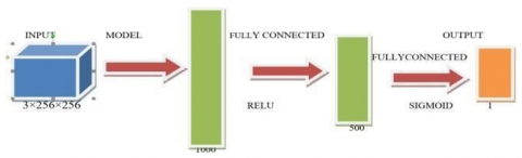
Three heterogeneous classifiers with high recall and accuracy are taken. Three pre-trained DL models were considered viz... RESNET-50-1, EfficientNetB3-1 and Densenet121-1. Each model forms three base classifiers. Figure 1 shows pre-trained DL model with one fully-connected layer. The (3×256×256) input is mapped to a column vector of 1000 rows. This column vector is converted another column vector having number of rows equal to number of classes (two in this case). Here sigmoid activation function is used. To avoid over fitting of model, a dropout layer is incorporated.
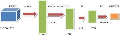
As shown in Figure 2 the other base classifier is designed with two fully connected layers. The (3×256×256) input is mapped to a column vector of 1000 rows and later converted into 500 rows and uses a Relu activation function. This column vector is converted another column vector having number of rows equal to number of classes (two in this case). Here sigmoid activation function is used. A dropout layer is used in this part also. As shown in Figure 3 the other base classifier is designed with three fully connected layers. The (3×256×256) input is mapped to a column vector of 1000 rows and later converted into 500 rows later 250 rows and uses a Relu activation function. This column vector is converted another column vector having number of rows equal to number of classes (two in this case). Here sigmoid activation function is used. A dropout layer is used in this part also. Figure 4 shows the proposed architecture in which RESNET-50-1, EfficientNetB3-1 and Densenet121-1 architecture outputs are applied to the meta layer, average of the predictions is done at meta layer [23, 24].
Figure 1. Base model with one fully connected layer
Figure 2. Base model with two fully connected layers
Figure 3. Base model with three fully connected layers
Figure 4. Proposed deep stacked ensemble
5.1 Dataset and data augmentation techniques
The proposed deep stacked ensemble was evaluated on Camelyon17 challenge Data set: This dataset has 400 whole slide images (WSI) collected from different medical centers [25]. The dataset consists of tumor slides which have metastases, normal slides and test slides which may or not have metastases.
Sample image is shown in Figure 5(a), the red colour indicates the cancer cells and Figure 5 (b) indicates the process of obtaining patches from WSI. The dataset is available at https://camelyon17.grand-challenge.org/Data.
Figure 5(a). Whole slide image
Figure 5(b). Process of obtaining patches from WSI
5.2 Model training and classification process
For training, first in the models data augmentation is used to increase the number of samples and the input images are pre- processed as per the model requirement. Then the pre- processed images are applied to the base model of the architecture followed by the global average pooling. Finally applied to the prediction layer with sigmoid activation function whose value exists in the range of (0,1). Trained the model over 3 different network architectures viz., ResNet50, Efficient Net B3 and DenseNet 121, with different number of fully connected layers, 1, 2 and 3. Here global average pooling (GAP) layer performs the average of each feature from the previous layers. The use of GAP reduces or avoids over fitting problem.
For prediction the sliding window technique is used with a window size of 64x64 to perform prediction over the entire image/slide. For each window over the slide, prediction of the probability of having cancer or tumor is done. After that it will verify whether the prediction probability is below or above the threshold value chosen. For example, if the threshold value is
0.5 i.e., if prediction value is above 0.5 then it will be considered as the slide has metastasis or else not. Based on the classified prediction values, the heatmap is obtained which provides the information regarding the presence of the tumor in the slide. Based on the heatmap classification was done. For efficient training DL models need large datasets. Size of the data set can be enlarged with the data augmentation techniques, used techniques in this paper were given below.
Initially batch size was taken as for and after doubled till memory error was faced. As the size of the batch increases memory requirement also increases. Finally, batch size was chosen to satisfy the memory condition.
In this experiment number of epochs taken were 30, 1e-3 as learning rate and 16 as batch size
5.3 Evaluation Metrics for Proposed Architecture
TN=True Negatives TP=True Positives FP=False Positives FN=False Negatives
P=TP / TP+FP
R=TP / TP+FN
F1 Score=(2×P×R)/ P+R
A=TP+TN / TP+FP+FN+TN
6.1 Analysing the performance of architectures
The evaluation of the model was done on CAMELYON 17 challenge dataset containing lymph node WSI of BC patients. The notation used is: a) Model-1 denotes the model with a single fully connected layer and a sigmoid layer b) Model-2 is the model with two fully connected layers along with a sigmoid layer, and c) Model-3 is the model with three fully connected layers along with a sigmoid layer. The: ResNet-50, DenseNet-121 and Efficient net- B3 are different models used. Total 9 base classifiers are formed with three DL models, among 9, three heterogeneous base classifiers are selected based on high recall in each DL model to form deep stacked ensemble. Desnet121-1, EfficientNetB3-1 and ResNet50-1 were selected. Figure 4 shows the deep Stacked Ensemble implementation.
****Algorithm to select base models for deep stacked Ensemble****
Input: Pretrained Models base 1, base2 and base 3 r1, r2, r3- Metrics of three ResNet models
d1, d2, d3- Metrics of three DenseNet models e1, e2, e3- Metrics of three EfficientNet models
The proposed model could correctly classify 1310 i.e., 1132 as true positives and 178 as true negatives patches out of the 1394
patches. Thus, for the proposed model, the accuracy and F1 score are 0.9613 and 0.8837, respectively. Table 1 presents experimental results of the proposed model, and that of heterogeneous base classifiers. The observations for the experiments conducted on CAMELYON 17 Dataset [25] are also presented. From Table 1 it is observed that the recall of the proposed model is higher than all base classifiers. Also, when compared to base classifiers the F1 score for this model is also high.
Table 1. The experiment results for the proposed model
|
Model |
Metrics |
|||||
|
AUC |
Loss |
Accuracy |
Recall |
Precision |
F1-Score |
|
|
Desnet121-1 |
0.9769 |
0.1583 |
0.9397 |
0.9082 |
0.7295 |
0.8091 |
|
EfficientNetB3-1 |
0.9688 |
0.1566 |
0.9497 |
0.8622 |
0.8478 |
0.8549 |
|
ResNet50-1 |
0.9711 |
0.1086 |
0.9684 |
0.8214 |
0.8471 |
0.8340 |
|
Proposed deep stacked Ensemble-Recall |
0.9586 |
0.1157 |
0.9613 |
0.9103 |
0.8586 |
0.8837 |
Figure 6(a). Confusion matrix of deep stacked ensemble
Figure 6(b). Generated AUC by stacking ensemble
Figure 7(a). Confusion matrix of ensemble for precision
Figure 7(b). Generated AUC by ensemble for precision
Figure 6(a) shows the Confusion Matrix for Ensemble for recall has less false negatives predictions compared to remaining models for 0.5 threshold for given dataset.
Figure 6(b) shows the Area Under the Curve for Stacking Ensemble for recall has high true positive rate when false positive rate as low.
Figure 7(a) shows the Confusion Matrix for Ensemble for Precision, has less false positive predictions compared to remaining models for 0.5 threshold for given dataset.
Figure 7(b) shows the Area Under the Curve for Stacking Ensemble has high true positive rate when false positive rate as low.
Table 2. The experiment results for the ensemble model precision
|
Model |
Metrics |
|||||
|
AUC |
Loss |
Accuracy |
Recall |
Precision |
F1-Score |
|
|
Desnet121-3 |
0.9610 |
0.1235 |
0.9663 |
0.8367 |
0.9162 |
0.8746 |
|
EfficientNetB3-3 |
0.9373 |
0.2594 |
0.9613 |
0.8112 |
0.9034 |
0.8548 |
|
ResNet50-2 |
0.9696 |
0.1307 |
0.9613 |
0.7653 |
0.8494 |
0.8052 |
|
Ensemble-Precision |
0.9624 |
0.1444 |
0.9648 |
0.8010 |
0.9401 |
0.8650 |
Table 2 presents experimental results of the model for precision, and that of heterogeneous base classifiers. From Table 2 it is observed that the precision of the model is higher than all base classifiers.
6.2 Performance analysis of the base classifiers
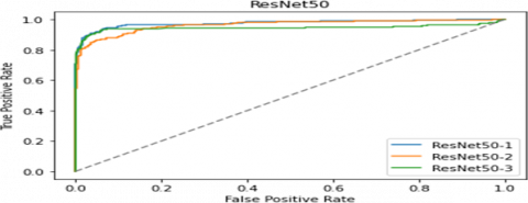
Figure 8 shows the Area Under the Curve for ResNet-50 with fully connected layer as 1 has high true positive rate when false positive rate as low.
Figure 9 shows the Area Under the Curve for DenseNet121 with fully connected layer as 2 has high true positive rate when false positive rate as low.
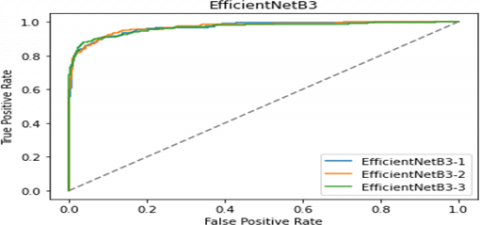
Figure 10 shows the Area Under the Curve for Efficient Net B3with fully connected layer as 2 has high true positive rate when false positive rate as low.
Figure 8. Generated AUC by ResNet-50architecture with fully connected layers as 1, 2 and 3
Figure 9. Generated AUC by DenseNet121 architecture with fully connected layers as 1, 2 and 3
Figure 10. Generated AUC by Efficient Net B3architecture with fully connected layers as 1, 2 and 3
Table 3. Performance analysis of ResNet-50 architecture with fully connected layers as 1, 2 and 3
|
Model |
Metrics |
|||||
|
AUC |
Loss |
Accuracy |
Recall |
Precision |
F1-Score |
|
|
ResNet50- |
0.971 |
0.108 |
0.968 |
0.821 |
0.847 |
0.83 |
|
1 |
4 |
|||||
|
ResNet50- |
0.969 |
0.130 |
0.961 |
0.765 |
0.849 |
0.80 |
|
2 |
5 |
|||||
|
ResNet50- |
0.963 |
0.133 |
0.960 |
0.760 |
0.849 |
0.80 |
|
3 |
2 |
|||||
Table 4. Performance analysis of Efficient Net B3architecture with fully connected layers as 1, 2 and 3
|
Model |
Metrics |
|||||
|
AUC |
Loss |
Accuracy |
Recall |
Precision |
F1-Score |
|
|
EfficientNetB 3-1 |
0.9688 |
0.1566 |
0.9497 |
0.8622 |
0.8478 |
0.8549 |
|
EfficientNetB 3-2 |
0.9570 |
0.1808 |
0.9577 |
0.8112 |
0.8785 |
0.8435 |
|
EfficientNetB 3-3 |
0.9373 |
0.2594 |
0.9613 |
0.8112 |
0.9034 |
0.8548 |
Table 3 shows the Performance analysis of ResNet-50 all three architectures, ResNet-50with fully connected layers as 1 has the superior performance than other two in accuracy, recall and F1 score.
Table 4 shows the Performance analysis of Efficient Net B3all three architectures, Efficient Net B3with fully connected layers as 1 has the superior performance in Recall than other two. Efficient Net B3with fully connected layers as 3 has the superior performance in Accuracy and Precision than other two.
Table 5. Performance analysis of DenseNet121 architecture with fully connected layers as 1, 2 and 3
|
Model |
Metrics |
|||||
|
AUC |
Loss |
Accuracy |
Recall |
Precision |
F1-Score |
|
|
Desnet1 21-1 |
0.976 |
0.158 |
0.939 |
0.908 |
0.729 |
0.809 |
|
Desnet1 21-2 |
0.978 |
0.113 |
0.960 |
0.852 |
0.865 |
0.858 |
|
Desnet1 21-3 |
0.961 |
0.123 |
0.966 |
0.836 |
0.916 |
0.874 |
Table 5 shows the Performance analysis of DenseNet121 all three architectures, DenseNet121 with 1 fully connected layers as has the superior performance in recall than other two. DenseNet121 with fully connected layers as 3 has the superior performance in Accuracy, Precision and F1 score than other two.
Table 6 shows Performance Comparisons of individual base models and stacking Ensemble architectures, deep stacked Ensemble has superior performance in recall and F1 score with 0.910 and 0.883. Ensemble for precision has high precision than other architectures, but here tradeoff between recall and precision was observed. ResNet50-1 has superior performance in accuracy than other models with 0.968.
Table 6. Performance comparisons of individual base models and stacking ensemble
|
Model |
Metrics |
|||||
|
AUC |
Loss |
Accuracy |
Recall |
Precision |
F1-Score |
|
|
ResNet50-1 |
0.971 |
0.108 |
0.968 |
0.821 |
0.847 |
0.834 |
|
ResNet50-2 |
0.969 |
0.130 |
0.961 |
0.765 |
0.849 |
0.805 |
|
ResNet50-3 |
0.963 |
0.133 |
0.960 |
0.760 |
0.849 |
0.802 |
|
EfficientNet B3-1 |
0.968 |
0.156 |
0.949 |
0.862 |
0.847 |
0.854 |
|
EfficientNet B3-2 |
0.950 |
0.180 |
0.957 |
0.811 |
0.878 |
0.843 |
|
EfficientNet B3-3 |
0.937 |
0.259 |
0.961 |
0.811 |
0.903 |
0.854 |
|
Desnet121-1 |
0.976 |
0.158 |
0.939 |
0.908 |
0.729 |
0.809 |
|
Desnet121-2 |
0.978 |
0.113 |
0.960 |
0.852 |
0.865 |
0.858 |
|
Desnet121-3 |
0.961 |
0.123 |
0.966 |
0.836 |
0.916 |
0.874 |
|
Deep stacked Ensemble-Recall |
0.958 |
0.115 |
0.961 |
0.910 |
0.858 |
0.883 |
|
Ensemble- Precision |
0.962 |
0.144 |
0.964 |
0.801 |
0.940 |
0.865 |
|
Mobile Net V2 |
0.869 |
- |
0.929 |
0.919 |
0.930 |
- |
Minimization of false negatives is vital to predict the metastasis in the BC patients. In view of this, a deep stacked ensemble model is proposed in this paper. To design this pre- trained DL models with variable number of fully connected layers are used. This is done to achieve high recall and accuracy in prediction of the metastasis in the BC patients. Resnet-50, Dense Net 121, and Efficient Net-B3 models were used to develop deep stacked ensemble with systematic approach. The performance of proposed deep stacked ensemble model is observed to be higher than the base classifiers. Additionally, high recall is achieved on CAMELYON 17 dataset. The recall and precision trade-off were also observed. Further to reduce false positives and false negatives, weighted average of stacking ensemble and also boosting ensemble may be done.
[1] World Health Organization. Accessed: October 18, 2021. Available: https://www.who.int/news-room/fact- sheets/detail/cancer.
[2] Cancer Symptoms and Causes. Mayo Clinic. Accessed: October 18, 2021. Available: https://www.mayoclinic.org/diseases-conditions/cancer/symptoms-causes/syc-20370588
[3] LeCun, Y., Bengio, Y., Hinton, G. (2015). Deep learning. Nature, 521(7553): 436-444. https://doi.org/10.1038/nature14539
[4] Albawi, S., Mohammed, T.A., Al-Zawi, S. (2017). Understanding of a convolutional neural network. In 2017 international conference on engineering and technology (ICET), Antalya, Turkey, pp. 1-6. https://doi.org/10.1109/ICEngTechnol.2017.8308186
[5] Xue, D., Zhou, X., Li, C., Yao, Y.D. (2020). An application of transfer learning and ensemble learning techniques for cervical histopathology image classification. IEEE Access, 8: 104603-104618. https://doi.org/10.1109/ACCESS.2020.2999816
[6] Shahidi, F., Daud, S.M., Abas, H., Ahmad, N.A., Maarop, N. (2020). Breast cancer classification using deep learning approaches and histopathology image: A comparison study. IEEE Access, 8: 187531-187552. https://doi.org/10.1109/ACCESS.2020.3029881
[7] Li, Z., Zhang, J., Tan, T., Teng, X.C. (2020). Deep learning methods for lung cancer segmentation in whole-slide histopathology images—the acdc@ lunghp challenge 2019. IEEE Journal of Biomedical and Health Informatics, 25(2): 429-440. https://doi.org/10.1109/JBHI.2020.3039741
[8] Wang, J., Liu, Q., Xie, H., Yang, Z., Zhou, H. (2021). Boosted efficientnet: Detection of lymph node metastases in breast cancer using convolutional neural networks. Cancers, 13(4): 661. https://doi.org/10.3390/cancers13040661
[9] Wang, L., Song, T., Katayama, T., Jiang, X., Shimamoto, T., Leu, J.S. (2021). Deep regional metastases segmentation for patient-level lymph node status classification. IEEE Access, 9: 129293-129302. https://doi.org/10.1109/ACCESS.2021.3113036
[10] Lin, H., Chen, H., Graham, S., Dou, Q., Rajpoot, N., Heng, P.A. (2019). Fast scannet: Fast and dense analysis of multi-gigapixel whole-slide images for cancer metastasis detection. IEEE transactions on medical imaging, 38(8): 1948-1958. https://doi.org/10.1109/TMI.2019.2891305
[11] Zheng, X., Yao, Z., Huang, Y, Yu, Y.Y., Wang, Y. (2020). Deep learning radiomics can predict axillary lymph node status in early-stage breast cancer. Nature communications, 11(1): 1236. https://doi.org/10.1038/s41467-020-15027-z
[12] Hu, Y., Su, F., Dong, K., Wang, C.Y., Zhao, X.Y. (2021). Deep learning system for lymph node quantification and metastatic cancer identification from whole-slide pathology images. Gastric Cancer, 24: 868-877. https://doi.org/10.1007/s10120-021- 01158-9
[13] Das, K., Conjeti, S., Chatterjee, J., Sheet, D. (2020). Detection of breast cancer from whole slide histopathological images using deep multiple instance CNN. IEEE Access, 8: 213502-213511. https://doi.org/10.1109/ACCESS.2020.3040106
[14] Hirra, I., Ahmad, M., Hussain, A., Ashraf, M.U., Saeed, I.A. (2021). Breast cancer classification from histopathological images using patch-based deep learning modeling. IEEE Access, 9: 24273-24287. https://doi.org/10.1109/ACCESS.2021.3056516
[15] Wang, S., Zhou, Y., Qin, X., Nair, S., Huang, X., Liu, Y. (2020). Label-free detection of rare circulating tumor cells by image analysis and machine learning. Scientific reports, 10(1): 12226. https://doi.org/10.1038/s41598-020-69056-1
[16] He, B., Lu, Q., Lang, J., Hai Yu, Peng, C., Bing, P.P. (2020). A new method for CTC images recognition based on machine learning. Frontiers in Bioengineering and Biotechnology, 8: 897. https://doi.org/10.3389/fbioe.2020.00897
[17] Jangam, E., Annavarapu, C.S.R. (2021). A stacked ensemble for the detection of COVID-19 with high recall and accuracy. Computers in Biology and Medicine, 135: 104608. https://doi.org/10.1016/j.compbiomed.2021.104608
[18] Mehra, R. (2018). Breast cancer histology images classification: Training from scratch or transfer learning? ICT Express, 4(4): 247-254. https://doi.org/10.1016/j.icte.2018.10.007
[19] Schmidt, A., Silva-Rodríguez, J., Molina, R., Naranjo, V. (2022). Efficient cancer classification by coupling semi supervised and multiple instance learning. IEEE Access, 10: 9763-9773. https://doi.org/10.1109/ACCESS.2022.3143345.
[20] Marini, N., Otálora, S., Müller, H., Atzori, M. (2021). Semi-supervised training of deep convolutional neural networks with heterogeneous data and few local annotations: An experiment on prostate histopathology image classification. Medical image analysis, 73: 102165. https://doi.org/10.1016/j.media.2021.102165
[21] Chen, Z., Chen, Z., Liu, J., Zheng, Q., Zhu, Y., Zuo, Y.F. (2020). Weakly supervised histopathology image segmentation with sparse point annotations. IEEE Journal of Biomedical and Health Informatics, 25(5): 1673-1685. https://doi.org/10.1109/JBHI.2020.3024262
[22] Xue, D., Zhou, X., Li, C., et al. (2020). An application of transfer learning and ensemble learning techniques for cervical histopathology image classification. IEEE Access, 8: 104603-104618. https://doi.org/10.1109/ACCESS.2020.2999816
[23] Shakeel, P.M., Tolba, A., Al-Makhadmeh, Z., Jaber, M.M. (2020). Automatic detection of lung cancer from biomedical data set using discrete AdaBoost optimized ensemble learning generalized neural networks. Neural Computing and Applications, 32, 777-790. https://doi.org/10.1007/s00521-018-03972-2
[24] Loddo, A., Buttau, S., Di Ruberto, C. (2022). Deep learning-based pipelines for Alzheimer's disease diagnosis: A comparative study and a novel deep-ensemble method. Computers in biology and medicine, 141: 105032. https://doi.org/10.1016/j.compbiomed.2021.105032
[25] CAMELYON17 contest home page. https://camelyon17.grand-challenge.org.