Jahida Subhedar![]() | Shabana Urooj
| Shabana Urooj![]() Anurag Mahajan*
Anurag Mahajan*![]()
© 2023 IIETA. This article is published by IIETA and is licensed under the CC BY 4.0 license (http://creativecommons.org/licenses/by/4.0/).
OPEN ACCESS
Optical Coherence Tomography (OCT) represents a non-invasive imaging modality capable of capturing high-resolution cross-sectional images of anatomical structures by scanning the tissue of interest in a transverse manner. Nevertheless, the inherent speckle noise present in OCT images considerably degrades their textural and sharpness qualities. Conventional wavelet-based modified soft thresholding methods have been employed to preserve pertinent information in denoising OCT images, but their performance remains contingent upon hyperparameter tuning. In this study, we introduce a Particle Swarm Optimization (PSO)-based optimized Wavelet Threshold (WT) method for OCT image denoising. By automating the process of determining hyperparameter values dependent on image quality, PSO streamlines the denoising process. The optimization problem's fitness function is defined by the Peak Signal-to-Noise Ratio (PSNR) parameter. To evaluate the WT-PSO algorithm, we utilized performance metrics such as Mean Square Error (MSE), PSNR, Structural Similarity Index Metrics (SSIM), and Contrast-to-Noise Ratio (CNR) on a publicly available dataset comprising 17 retinal OCT images. The proposed denoising approach demonstrates comparable results to those obtained by manual iterative or trial methods, delivering marginal improvements in performance parameters and image quality. Moreover, our method outperforms traditional wavelet-based state-of-the-art techniques for denoising OCT images, highlighting its potential for widespread application in the field.
optical coherence tomography, speckle noise, wavelet transform, particle swarm optimization, despeckling
Optical Coherence Tomography (OCT) imaging techniques, along with fundus imaging, play a vital role in diagnosing diseases in ophthalmology. OCT imaging is particularly useful for examining tissues of retinal layers and skin layers due to its penetrating capability. By utilizing a low coherence interferometer, OCT captures cross-sectional micro-level structural information about tissues, as illustrated in Figure 1. High-resolution images of internal micro-structures up to 1-2 mm in depth can be obtained using this imaging technique [1].
However, OCT images are inherently affected by speckle noise, which arises from the interference of transmitted and echo signals with coherent signal sources. Speckles can either carry structural information or act as noise that degrades image quality [2, 3]. Speckle noise, being multiplicative in nature, imparts a granular appearance to images, reduces contrast and resolution, and ultimately limits their analytical value [4]. The increasing accessibility and affordability of medical imaging technology has led to the generation of vast amounts of image data, which can be employed for Computer-Assisted Diagnosis (CAD) systems. High-quality images are essential for enhancing the performance of these CAD systems.
Traditional methods for reducing noise in OCT images include Mean, Median, Wiener, and Bilateral filtering [5]. However, these approaches often cause over-smoothing, resulting in the loss of structural information. To avoid over-smoothing at image edges, the Total Variation Denoising (TVD) method was proposed [6].
Figure 1. A typical retinal OCT image with 10 segmented layers [7]
Although TVD preserves edges, it may lead to texture over-smoothing and a staircase effect. Transform domain filtering methods, such as wavelet transform, curvelet-based [8], contourlet-based [9], and Gaussianization transform [10], incorporating various shrinkage techniques, have proven more effective at preserving structural information. In studies by Zaki et al. [11] and Chen [12], noise-adaptive wavelet filtering for sub-bands was proposed by decomposing images into four sub-bands using wavelet transform. Each of the aforementioned methods offers its own advantages, and combining them can yield improved results. Techniques like the modified total variation method with wavelet algorithm, the total variation method with shearlet transform, and the Block matching 3D-based Total Variation [13] have been investigated to enhance speckle reduction, texture preservation, and edge preservation. However, the performance of these methods declines as noise levels increase.
Deep learning methods have also been explored for noise reduction in OCT images while preserving structural information and texture [14, 15]. These methods necessitate a significant amount of labeled data, which is both time-consuming and laborious to obtain. Acquiring databases with ground truth remains a challenge. CNN-based denoising models tend to have complex structures with numerous parameters that need to be tuned for optimal performance and to prevent over-fitting.
Among the various wavelet despeckling approaches, like hard thresholding, soft thresholding and modified soft thresholding, modified soft thresholding functions have been demonstrated to yield the best results for speckle noise removal while retaining structural information [16-21]. The modified soft thresholding function relies on three tuning parameters: the degree of curvature (β), the degree of shrinkage of high-frequency coefficients (α), and the threshold value (K). These parameter values determine the level of artifacts in the reconstructed image, preservation of edge information, and the threshold for speckle filtering. Appropriate values for these hyperparameters must be set to achieve balanced performance. Traditionally, these values are determined manually by testing the algorithm with different sets of hyperparameters. Given that hyperparameter values yielding high-quality denoised images vary based on input noisy image characteristics (e.g., image quality, scaling, orientation, intensity distribution), an automated method for setting these values based on image quality is necessary.
In this paper, we propose a Particle Swarm Optimization (PSO)-based wavelet filtering algorithm to automatically set hyperparameter values based on image quality and obtain high-quality denoised images. PSNR is employed as a fitness function for PSO. The PSO-based WT algorithm effectively denoises retinal OCT images, achieving results similar to those obtained using non-PSO methods. The algorithm improves PSNR values and the SSIM parameter, which measures the preservation of structural information in denoised images. The paper is structured as follows: Section 2 presents materials and methods, Section 3 discusses results, and Section 4 offers conclusions.
The block diagram of the implemented PSO-WT (Particle Swarm Optimization based modified soft thresholding Wavelet Transform) method is shown in Figure 2.
Figure 2. Block diagram of proposed PSO based modified soft thresholding for OCT image denoising
The noisy retinal OCT image (z) is input to the log transform block which convert multiplicative speckle noise into additive noise. By using log transforming the image we can use near additive models which are simpler to work [10]. So, followed the similar approaches as in studies [8, 10, 17, 19]. The 2D discrete wavelet transform (DWT) is taken to obtain approximation (low-frequency sub-band) and detailed coefficient (high-frequency sub-band data) representation of the input image data (z) of size N×N. The size of each coefficient matrix is (N/2×N/2), i and j are used for coefficient matrix indexing.
$\mathrm{y}=$ 2D_DWT(z) $=\left(y_{\mathrm{i} . \mathrm{j}}^{L L}, y_{\mathrm{i} . \mathrm{j}}^{L H}, y_{\mathrm{i} . \mathrm{j}}^{H L}, y_{\mathrm{i} . \mathrm{j}}^{H H}\right)$ (1)
The detailed wavelet coefficients are filtered using the modified threshold function given by Cao et al. [19]. It incorporates three hyper-parameters that decide the degree of curvature (β), degree of shrinkage of high frequency coefficient (α), and threshold value (K). The modified wavelet coefficients are obtained using Eqns. (2) and (3):
$\tilde{y}_{i, j=1}\left\{\begin{array}{cc}x_{i, j}+\frac{2}{\pi} \tan ^{-1}\left(\beta \frac{x_{i, j}}{T h}+\operatorname{sgn}\left(y_{i . j}\right) \alpha\right) y_{t h},\left|y_{i, j}\right| \geq y_{t h} \\ \frac{2}{\pi} \tan ^{-1}(\alpha) y_{i, j},|y i, j|<y_{t h}\end{array}\right.$ (2)
x(i,j) is calculated by adding or subtracting the threshold value from the wavelet coefficient depending on whether y is greater than or less than yth. The threshold value is calculated by:
$y_{t h}=K \frac{m d n\left(\left|H H_{10 c t}\,\,\right|\right)}{0.6754} \frac{\sqrt{2 \ln M}}{L_d}$ (3)
where, d is the decomposition level of the wavelet transform, Lddepends on decomposition level. M is the length of the signal.
The quality of denoised images depends on the values set for the three hyper parameters in Eqns. (2) and (3). We have used Particle Swarm Optimization (PSO) algorithm to optimize hyper-parameter values with PSNR as the fitness function. PSO mimics navigation logic followed by a flock of birds. It is used to find the optimum solution while maximizing or minimizing function value. Particles represent a bird’s population [22].
$P_i=\left\{\alpha_i, \beta_i, K_i\right\}$ (4)
Every particle starts with random values of hyper-parameters in different directions. Particles move in the problem space following a set of rules. The image is reconstructed by inverse 2D DWT and inverse log transform for every particle and all the iterations. The fitness value i.e., PSNR of each particle solution is computed between input noisy image and reconstructed image.
$Fitness$ $=P S N R_{p i}$ (5)
If the particles fitness (FitnessPi) value is greater than the particle best (Pbest) so far then, particle best value is modified. In case the particles fitness (FitnessPi) value is greater than the global fitness (Gbest) value, the global value is modified. Then, the velocity and position (value) of the particles are updated for the next round of iteration.
For modified soft thresholding scheme each particle position (value) is comprises three parameters (α), (β) and k. Hence Eqns. (6) and (7) are used to modify the velocity and value of α for next iteration.
$\begin{array}{r}v_{-} \alpha_i^{i t r+1}=w v_{-} \alpha_i^{i t r}+c 1 r 1\left(\text {Pbest}_{\alpha_i}-\alpha_i^{i t r}\right) \\ +c 2 r 2\left(\text { Gbest_} \alpha_i-\alpha_i^{i t r}\right)\end{array}$ (6)
$\alpha_i^{i t r+1}=\alpha_i^{i t r}+v_{-} \alpha_i^{i t r 1+1}$ (7)
where, c1, c2 are acceleration coefficients, itr is the number of iterations the particles would undergo, and w is inertia weight. The r1 and r2 are random numbers used to set the initial values of tuning parameters and $v_{-} \alpha_i^{i t r+1}$ is the velocity for ithα particle in next iteration.
The Eqns. (8) and (9) are used to modify the velocity and value of β:
$\begin{aligned} v_{\beta_i^{i t r+1}}\,\,=w v_{\beta_i^{i t r}} & +c 1 r 1\left(\text { Pbest}_{\beta_i}-\beta_i^{i t r}\right) +c 2 r 2\left(\text { Gbest_} \beta_i-\beta_i^{i t r}\right)\end{aligned}$ (8)
$\beta_i^{i t r+1}=\beta_i^{i t r}+v_{-} \beta_i^{i t r 1+1}$ (9)
and Eqns. (10) and (11) for modifying k for next iteration.
$\begin{aligned} & v_{-} k_i^{i t r+1}=w v_{-} k_i^{i t r}+c 1 r 1\left(\text { Pbest}_{k_i}-k_i^{\mathrm{itr}}\right) \\ &+\mathrm{c} 2 \mathrm{r} 2\left(\text { Gbest_} \mathrm{k}_{\mathrm{i}}-\mathrm{k}_{\mathrm{i}}^{\mathrm{itr}}\right)\end{aligned}$ (10)
$k_i^{i t r+1}=k_i^{i t r}+v_{-} k_i^{i t r 1+1}$ (11)
The PSO algorithm is executed for several iterations. The final optimized solution for three hyper-parameter which maximizes the PSNR is obtained. The optimized values of hyper-parameters α, β, and k using PSO to give better performance may be different for different images, based on image quality, scaling, the orientation of image and intensity distribution, etc. Thus, the proposed system provides automation of hyperparameter tuning for modified soft thresholding wavelet denoising approach, irrespective of image the main steps of algorithm are stated in Algorithm.
Algorithm: Modified soft threshold wavelet transform with PSO for OCT image denoising
|
1: Read image 2: Convert image into log domain 3: Take 2D discrete wavelet transform 4: Num of iterations, itr % initializations of algorithm parameters 5: Num of particles n 6: initialize array for n α particles with random values (Positions) 7: initialize array for n β particles with random values (positions) 8: initialize array for n k particles with random values (Positions) 9: initialize array for Pbest for n particles 10: initialize Gbest value 11: initial velocities for α, β, and k 12: assign values for learning factors c1, c2, weight w, r1 and r2. 13: for j=1 to itr do 14: for i=1 to n do 15: detailed wavelet coefficient matrix filtering using Eqns. (2) and (3) 16: image reconstruction using inverse DWT. 17: compute PSNR as a fitness function value for PSO. 18: if fitness > Pbest then 19: Pbest=fitness 20: update particles best α, particles best β, and particles best k to current iteration values α, β, and k. 21: end if 22: if fitness > Gbest then 23: Gbest=fitness 24: update global best α, β, and k to current iteration values α, β, and k. 25: end if 26: update value of α for next iteration using Eqns. (6) and (7) 27: update value of β for next iteration using Eqns. (8) and (9) 28: update value of k for next iteration using Eqns. (10) and (11) 29: end for 30: end for |
The performance of the proposed method for retinal OCT images is evaluated using parameters MSE, PSNR, SSIM, and CNR.
MSE (Mean squre Error): This is a basic parameter used to compare the original noisy image(z) and denoised image (d), and N total number of pixels.
$\mathrm{MSE}=\frac{1}{N} \sum_{j=1}^N\left(Z_j-D_J\right)^2$
PSNR (Peak signal to noise ratio): When SNR is expressed with reference to the maximum power of intensity within the image, it is referred to as PSNR.
$\mathrm{PSNR}=20 \log _{10} \frac{\left(\mathbf{2}^{\mathrm{B}}-\mathbf{1}\right)}{\sqrt{\mathrm{MSE}}}$
where, B is the number of bits per pixel and $2^B-1$ is the maximum value of gray level.
Contrast to Noise Ratio (CNR): This is a patch/window-based parameter. This gives a contrast relationship between background and image features. It specifies the ability to visualize the image features in a noisy environment:
$\mathrm{CNR}=\frac{1}{\mathrm{~F}} \sum_{\mathrm{f}=1}^{\mathrm{f}=\mathrm{F}} \frac{\left|\mu_{\mathrm{f}}-\mu_{\mathrm{b}}\right|}{\sqrt{\left|\sigma_{\mathrm{f}}^2-\sigma_{\mathrm{b}}^2\right|}}$
where, μb and $\sigma_{\mathrm{b}}^2$ are mean and the variance of background image, μf and $\sigma_f^2$ are mean and the variance of patches of foreground image.
Structural similarity index (SSIM): SSIM gives the structural relationship between the original image and the denoised image. This parameter justifies the human visual system more closely than PSNR. SSIM compares the two images based on luminance, contrast, and structure parameters.
$\operatorname{SSIM}=\frac{\left(2 \mathrm{u}_{\mathrm{z}} u_{\mathrm{d}}+\mathrm{b} 1\right)\left(2 \sigma_{\mathrm{zd}}\,+\,\mathrm{b} 2\right)}{\left(\mathrm{u}_{\mathrm{z}}^2\,+\mathrm{u}_{\mathrm{d}}^2\,+\mathrm{b} 1\right)\left(\sigma_{\mathrm{z}}^2\,+\sigma_{\mathrm{d}}^2+\mathrm{b} 2\right)}$
where, μz, σz, are the mean, standard deviation of noisy input image, μd and σd are the mean, standard deviation of denoised image(d). σzd is cross-covariance for input noisy image(z) and denoised image(d). b1 and b2 are constants calculated from dynamic range of pixxel values.
In implementation the SSIM function from MATLAB is used with all default parameters values except dynamic range and radius. Dynamic range is calculated from the denoised image, and the radius value is kept at 2.
The data-set used for testing the algorithms was used in study [23]. The data-set consists of 17 retinal OCT images, of which ten images are of normal subjects, and seven are from AMD (age-related macular degeneration) subjects. The algorithm is implemented in MATLAB R2017a, the system with Intel Core i5-7200U CPU, 2.50 GHz, and 8 GB RAM.
For wavelet transform, the wavelet family used is Daubechies (db2), and implemented decomposition level is 1. Cao et al. [19] implemented the modified soft thresholding algorithm for the skin OCT data-set, therefore, to compare the performance, we have implemented the modified soft thresholding [19] method with decomposition level 1 for retinal OCT images.
The hyperparameter variations are set within limits [19] (alpha=0-0.5, beta 1 to 5, and k=1 to 1.5). To provide a large number of combinations of values of α, β, and k number of particles is set to 100, and by observations during the experimentations, the number of iterations is fixed to 15 when the PSNR value almost becomes stable.
As performance of wavelet based denoising approach can be improved by changing the threshold selection method, hard thresholding to soft thresholding, reducing the effect of Gibbs phenomena [19]. Then as speckle can be noise or carrier of useful information, useful information can be preserved by modified soft thresholding method. Its effectiveness depends on combination of hyper parameter values α, β, and k. We have automated the process of setting these parameters which is independent of quality of noisy input images.
The values of α, β, and k that perform better denoising differ for different images. Finding these values manually by the trial method is not the convenient way every time input image characteristics (like the quality of the image, Scaling, the orientation of the image, intensity distribution, etc.). are changed, so the proposed method suggests an automated method of setting values of hyperparameter of modified soft thresholding-based denoising algorithm. The automated method of setting hyperparameters gives comparable results that would be obtained by the manual trial method. It is observed from the Tables 1-4 the performance parameters MSE, PSNR, SSIM, and CNR are improved marginally.
Table 1. Performance parameter: MSE
|
Method \image database |
Donoho hard thresholding [24] |
Donoho soft thresholding [18] |
Modified soft thresholding [19] |
PSO based wavelet thresholding (proposed) |
|
Image 1 |
362.29 |
206.88 |
160.0179 |
158.206 |
|
Image 2 |
316.11 |
184.36 |
142.9952 |
141.1112 |
|
Image 3 |
325.42 |
190.56 |
147.8231 |
146.2622 |
|
Image 4 |
293.73 |
170.01 |
133.6118 |
131.5868 |
|
Image 5 |
240.81 |
138.39 |
106.5273 |
105.7769 |
|
Image 6 |
296.11 |
178.18 |
139.3969 |
137.6856 |
|
Image 7 |
284.77 |
169.12 |
130.619 |
128.8745 |
|
Image 8 |
291.39 |
172.95 |
135.1155 |
133.8362 |
|
Image 9 |
352.04 |
209.11 |
161.9777 |
160.493 |
|
Image 10 |
354.88 |
201.70 |
156.8982 |
152.6841 |
|
Image 11 |
348.35 |
197.78 |
155.3355 |
153.7897 |
|
Image 12 |
347.00 |
194.22 |
152.2209 |
150.7548 |
|
Image 13 |
364.31 |
202.27 |
157.2588 |
155.799 |
|
Image 14 |
332.02 |
183.43 |
143.3578 |
140.825 |
|
Image 15 |
340.89 |
187.06 |
145.6276 |
143.8037 |
|
Image 16 |
334.00 |
186.87 |
144.7187 |
143.2287 |
|
Image 17 |
312.82 |
183.47 |
141.0186 |
139.5642 |
|
Mean MSE |
323.35 |
185.67 |
144.3835 |
142.6048 |
Table 2. Performance parameter PSNR
|
Method \image database |
Donoho hard thresholding [24] |
Donoho soft thresholding [18] |
Modified soft thresholding [19] |
PSO based wavelet thresholding (proposed) |
|
Image 1 |
22.54 |
24.97 |
26.0891 |
26.1386 |
|
Image 2 |
23.13 |
25.47 |
26.5776 |
26.6352 |
|
Image 3 |
23.00 |
25.33 |
26.4334 |
26.4795 |
|
Image 4 |
23.45 |
25.83 |
26.8724 |
26.9387 |
|
Image 5 |
24.31 |
26.72 |
27.8562 |
27.8869 |
|
Image 6 |
23.42 |
25.62 |
26.6883 |
26.7419 |
|
Image 7 |
23.59 |
25.85 |
26.9707 |
27.0291 |
|
Image 8 |
23.49 |
25.75 |
26.8238 |
26.8651 |
|
Image 9 |
22.66 |
24.93 |
26.0363 |
26.0762 |
|
Image 10 |
22.63 |
25.08 |
26.1746 |
26.2929 |
|
Image 11 |
22.71 |
25.17 |
26.2181 |
26.2615 |
|
Image 12 |
22.73 |
25.25 |
26.3061 |
26.3481 |
|
Image 13 |
22.52 |
25.07 |
26.1647 |
26.2052 |
|
Image 14 |
22.92 |
25.50 |
26.5666 |
26.644 |
|
Image 15 |
22.80 |
25.41 |
26.4984 |
26.5531 |
|
Image 16 |
22.89 |
25.42 |
26.5256 |
26.5705 |
|
Image 17 |
23.18 |
25.50 |
26.638 |
26.6831 |
|
Mean PSNR |
23.06 |
25.46 |
26.5552 |
26.6088 |
Table 3. Performance parameter SSIM
|
Method \image database |
Donoho hard thresholding [24] |
Donoho soft thresholding [18] |
Modified soft thresholding [19] |
PSO based wavelet thresholding (proposed) |
|
Image 1 |
0.50 |
0.59 |
0.6307 |
0.6394 |
|
Image 2 |
0.51 |
0.61 |
0.6417 |
0.6505 |
|
Image 3 |
0.51 |
0.60 |
0.6353 |
0.6436 |
|
Image 4 |
0.52 |
0.61 |
0.6471 |
0.657 |
|
Image 5 |
0.54 |
0.64 |
0.6832 |
0.6866 |
|
Image 6 |
0.52 |
0.60 |
0.6406 |
0.6499 |
|
Image 7 |
0.52 |
0.61 |
0.6462 |
0.6547 |
|
Image 8 |
0.52 |
0.61 |
0.6479 |
0.6547 |
|
Image 9 |
0.52 |
0.61 |
0.6491 |
0.6561 |
|
Image 10 |
0.52 |
0.61 |
0.6527 |
0.6617 |
|
Image 11 |
0.53 |
0.62 |
0.6615 |
0.6685 |
|
Image 12 |
0.51 |
0.61 |
0.6502 |
0.6568 |
|
Image 13 |
0.53 |
0.63 |
0.6662 |
0.6721 |
|
Image 14 |
0.51 |
0.61 |
0.6466 |
0.657 |
|
Image 15 |
0.51 |
0.61 |
0.6491 |
0.6576 |
|
Image 16 |
0.51 |
0.61 |
0.6443 |
0.6528 |
|
Image 17 |
0.51 |
0.60 |
0.6490 |
0.6505 |
|
Mean SSIM |
0.52 |
0.61 |
0.6490 |
0.6570 |
Table 4. Performance parameter CNR
|
Method \image database |
Donoho hard thresholding [24] |
Donoho soft thresholding [18] |
Modified soft thresholding [19] |
PSO based wavelet thresholding (proposed) |
|
Image 1 |
0.50 |
0.59 |
0.6307 |
0.6394 |
|
Image 2 |
0.51 |
0.61 |
0.6417 |
0.6505 |
|
Image 3 |
0.51 |
0.60 |
0.6353 |
0.6436 |
|
Image 4 |
0.52 |
0.61 |
0.6471 |
0.657 |
|
Image 5 |
0.54 |
0.64 |
0.6832 |
0.6866 |
|
Image 6 |
0.52 |
0.60 |
0.6406 |
0.6499 |
|
Image 7 |
0.52 |
0.61 |
0.6462 |
0.6547 |
|
Image 8 |
0.52 |
0.61 |
0.6479 |
0.6547 |
|
Image 9 |
0.52 |
0.61 |
0.6491 |
0.6561 |
|
Image 10 |
0.52 |
0.61 |
0.6527 |
0.6617 |
|
Image 11 |
0.53 |
0.62 |
0.6615 |
0.6685 |
|
Image 12 |
0.51 |
0.61 |
0.6502 |
0.6568 |
|
Image 13 |
0.53 |
0.63 |
0.6662 |
0.6721 |
|
Image 14 |
0.51 |
0.61 |
0.6466 |
0.657 |
|
Image 15 |
0.51 |
0.61 |
0.6491 |
0.6576 |
|
Image 16 |
0.51 |
0.61 |
0.6443 |
0.6528 |
|
Image 17 |
0.51 |
0.60 |
0.6490 |
0.6505 |
|
Mean CNR |
0.52 |
0.61 |
0.6490 |
0.6570 |
Table 5. Comparison of PSNR and SSIM [15] for MSBTD [25] (state of art method) and PSO based wavelet thresholding (proposed)
|
Method/Parameter |
MSBTD |
PSO based wavelet thresholding (proposed) |
|
Mean PSNR |
26.46 |
26.61 |
|
Mean SSIM |
0.56 |
0.66 |
In Table 5 gives comparison of for MSBTD [25] (state of art method) for OCT denoising which has used same dataset.
Time taken for execution for hard thresholding is 19 sec, for soft thresholding 17 sec and for modified soft thresholding 18 sec. Average time taken by MSBTD method for denoising one OCT B scan is around 9 minutes and for proposed method, it is around 179 sec.
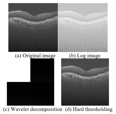
The OCT retinal image denoising is carried out for all 17 images in the database. The processing of one of the images (Image 4 from the database) is shown in Figure 3 below.
Figure 3. OCT retinal image processing using wavelet transforms (Image 4 from database)
The modified soft thresholding-based denoising algorithm preserves the finer details of images. Still, the performance depends on tuning parameters that affect artifacts, edge preservation in the reconstructed image, and filtering of speckles carrying information. It is observed that the use of PSO based tuning of parameters improves results marginally as compared to the same methods without PSO. The advantage here is that there is no need to manually find and set the hyper parameter values whenever quality of input image (due to Scaling, orientation of the image, intensity distribution, etc.) is changed.
The proposed method is implemented for denoising any OCT images of different characteristics and getting optimum PSNR (fitness function for PSO) value. In Future work, if any specific parameter is to be improved that can considered as fitness function and its effectiveness on overall performance can be tested. Also, effectiveness of the proposed denoising algorithm can be tested by segmentation or classification tasks using denoised OCT images for disease detection.
Princess Nourah bint Abdulrahman University Researchers Supporting Project number (PNURSP2023R79); Princess Nourah bint Abdulrahman University, Riyadh, Saudi Arabia.
[1] Xu, M., Tang, C., Hao, F., Chen, M., Lei, Z. (2020). Texture preservation and speckle reduction in poor optical coherence tomography using the convolutional neural network. Medical Image Analysis, 64: 101727. https://doi.org/10.1016/j.media.2020.101727
[2] Jain, L., Singh, P. (2022). A novel wavelet thresholding rule for speckle reduction from ultrasound images. Journal of King Saud University-Computer and Information Sciences, 34(7): 4461-4471. https://doi.org/10.1016/j.jksuci.2020.10.009
[3] Habib, W., Sarwar, T., Siddiqui, A.M., Touqir, I. (2017). Wavelet denoising of multiframe optical coherence tomography data using similarity measures. IET Image Processing, 11(1): 64-79. https://doi.org/10.1049/iet-ipr.2016.0160
[4] Liu, X., Ramella-Roman, J.C., Huang, Y., Guo, Y., Kang, J.U. (2013). Robust spectral-domain optical coherence tomography speckle model and its cross-correlation coefficient analysis. JOSA A, 30(1): 51-59. https://doi.org/10.1364/josaa.30.000051
[5] Shah, A.A., Malik, M.M., Akram, M.U., Bazaz, S.A. (2016). Comparison of noise removal algorithms on Optical Coherence Tomography (OCT) image. In 2016 IEEE International Conference on Imaging Systems and Techniques (IST), pp. 166-170. https://doi.org/10.1109/IST.2016.7738217
[6] Shamouilian, M., Selesnick, I. (2019). Total variation denoising for optical coherence tomography. In 2019 IEEE Signal Processing in Medicine and Biology Symposium (SPMB), pp. 1-5. https://doi.org/10.1109/SPMB47826.2019.9037832
[7] Yan, Q., Chen, B., Hu, Y., Cheng, J., Gong, Y., Yang, J., Liu, J., Zhao, Y. (2020). Speckle reduction of OCT via super resolution reconstruction and its application on retinal layer segmentation. Artificial Intelligence in Medicine, 106: 101871. https://doi.org/10.1016/j.artmed.2020.101871
[8] Jian, Z., Yu, Z., Yu, L., Rao, B., Chen, Z., Tromberg, B. J. (2009). Speckle attenuation in optical coherence tomography by curvelet shrinkage. Optics Letters, 34(10): 1516-1518. https://doi.org/10.1364/ol.34.001516
[9] Xu, J., Ou, H., Lam, E. Y., Chui, P.C., Wong, K.K. (2013). Speckle reduction of retinal optical coherence tomography based on contourlet shrinkage. Optics Letters, 38(15): 2900-2903. https://doi.org/10.1364/ol.38.002900
[10] Amini, Z., Rabbani, H. (2017). Optical coherence tomography image denoising using Gaussianization transform. Journal of Biomedical Optics, 22(8): 086011-086011. https://doi.org/10.1117/1.jbo.22.8.086011
[11] Zaki, F., Wang, Y., Su, H., Yuan, X., Liu, X. (2017). Noise adaptive wavelet thresholding for speckle noise removal in optical coherence tomography. Biomedical Optics Express, 8(5): 2720-2731. https://doi.org/10.1364/boe.8.002720
[12] Chen, H. (2021). Fusion denoising algorithm of optical coherence tomography image based on point-estimated and block-estimated. Optik, 225: 165864. https://doi.org/10.1016/j.ijleo.2020.165864
[13] Huang, S., Tang, C., Xu, M., Qiu, Y., Lei, Z. (2019). BM3D-based total variation algorithm for speckle removal with structure-preserving in OCT images. Applied Optics, 58(23): 6233-6243. https://doi.org/10.1364/ao.58.006233
[14] Chen, Z., Zeng, Z., Shen, H., Zheng, X., Dai, P., Ouyang, P. (2020). DN-GAN: Denoising generative adversarial networks for speckle noise reduction in optical coherence tomography images. Biomedical Signal Processing and Control, 55: 101632. https://doi.org/10.1016/j.bspc.2019.101632
[15] Kande, N.A., Dakhane, R., Dukkipati, A., Yalavarthy, P.K. (2020). SiameseGAN: A generative model for denoising of spectral domain optical coherence tomography images. IEEE Transactions on Medical Imaging, 40(1): 180-192. https://doi.org/10.1109/TMI.2020.3024097
[16] Chang, S.G., Yu, B., Vetterli, M. (2000). Adaptive wavelet thresholding for image denoising and compression. IEEE Transactions on Image Processing, 9(9): 1532-1546. https://doi.org/10.1109/83.862633
[17] Gupta, P.K., Lal, S., Husain, F. (2020). A robust framework for de-speckling of optical coherence tomography images. International Journal of Advanced Science and Technology, 29(5): 4094–4106.
[18] Donoho, D.L. (1995). De-noising by soft-thresholding. IEEE Transactions on Information Theory, 41(3): 613-627. https://doi.org/10.1109/18.382009
[19] Cao, J., Wang, P., Wu, B., Shi, G., Zhang, Y., Li, X., Zhang, Y., Liu, Y. (2018). Improved wavelet hierarchical threshold filter method for optical coherence tomography image de-noising. Journal of Innovative Optical Health Sciences, 11(03): 1850012. https://doi.org/10.1142/S1793545818500128
[20] Zhang, Y., Ding, W., Pan, Z., Qin, J. (2019). Improved wavelet threshold for image de-noising. Frontiers in Neuroscience, 13: 39. https://doi.org/10.3389/fnins.2019.00039
[21] Kaur, P., Singh, G., Kaur, P. (2018). A review of denoising medical images using machine learning approaches. Current Medical Imaging, 14(5): 675-685. https://doi.org/10.2174/1573405613666170428154156
[22] Wang, D., Tan, D., Liu, L. (2018). Particle swarm optimization algorithm: an overview. Soft Computing, 22: 387-408. https://doi.org/10.1007/s00500-016-2474-6
[23] Fang, L., Li, S., McNabb, R.P., Nie, Q., Kuo, A.N., Toth, C.A., Izatt, J.A., Farsiu, S. (2013). Fast acquisition and reconstruction of optical coherence tomography images via sparse representation. IEEE Transactions on Medical Imaging, 32(11): 2034-2049. https://doi.org/10.1109/TMI.2013.2271904
[24] Donoho, D.L., Johnstone, I.M. (1994). Threshold selection for wavelet shrinkage of noisy data. In Proceedings of 16th annual international conference of the IEEE Engineering in Medicine and Biology Society, pp. A24-A25. https://doi.org/10.1109/iembs.1994.412133
[25] Fang, L., Li, S., Nie, Q., Izatt, J. A., Toth, C.A., Farsiu, S. (2012). Sparsity based denoising of spectral domain optical coherence tomography images. Biomedical Optics Express, 3(5): 927-942. https://doi.org/10.1364/boe.3.000927