Myriam Hadjouni![]() | Hela Elmannai
| Hela Elmannai![]() | Aymen Saad
| Aymen Saad![]() | Ammar Altaher
| Ammar Altaher![]() | Ahmed Elaraby*
| Ahmed Elaraby*![]()
© 2023 IIETA. This article is published by IIETA and is licensed under the CC BY 4.0 license (http://creativecommons.org/licenses/by/4.0/).
OPEN ACCESS
Early detection of brain tumors (BTs) can save valuable lives. BTs classification is usually accomplished by using magnetic resonance imaging (MRI), which is commonly carried out earlier than definitive talent surgery. Machine learning (ML) strategies can assist radiologists to diagnose tumors barring invasive measures. One of the challenges of traditional classifiers is that they rely on informative hand-crafted features, which can be a time-consuming process to extract. We proposed fully automatic framework for BTs classification with weighted contrast-enhanced MRI images. The proposed framework includes an enhancement preprocessing to improve input images quality and a classification phase for images classification into three classes of tumors (meningioma, glioma and pituitary tumor) and ordinary cases. The model was built used “Lightweight Convolutional Neural Network (LWCNN)” that allows to automatically extract features. We tested the LWCNN model in two experiments. In the first one, the model has been tested with original datasets. We tested our proposed framework on the same dataset after enhancing the features of MRI images in the second experiment. As per the experiment results, it has been observed that the proposed framework achieves the desired outcome which demonstrates the effectiveness of our proposed framework.
deep learning (DL), lightweight convolutional neural networks (LWCNN), brain tumors (BTs), classification image
Billions of cells in human mind which makes evaluation very difficult. The central and peripheral nervous systems both include tumors that belong to the genetically, biochemically, and clinically diverse category known as pediatric brain tumors. In terms of incidence and mortality among pediatric malignancies, they are collectively the most frequent solid tumors in children and come in second place after leukemias. In USA, Individuals who are below 20 years of age are diagnosed with 2,200 intracranial pediatric brain tumors annually, accounting for 16.6% of all pediatric cancer diagnoses; 78% of these neoplasms are malignant in origin, while the other 21% are benign or have unknown behavior [1]. About 52% of these malignancies comprise astrocytoma, 21% are primitive neuroectodermal tumors (PNET), 15% are other gliomas, while 9% are ependymomas [1]. Another 6-10% of all pediatric cancers are neuroblastomas (NB), It is the most commonly occurring solid extracranial tumor of the nervous system, which develop in sympathetic ganglia and adrenal medulla that new cases account for around 650 in children per year in USA [2].
These extracranial tumors affect infants under the age of two in close to 50% of cases [3]. There is a possibility that these tumors have an origin that conflicts with some conventional wisdom on tumor development, considering the fact that most Pediatric brain tumors (PBTs) in children occur at a young age. The conventional wisdom that most malignancies take at least ten years to form. In fact, current studies are starting to point to an etiology that involves the interaction of early environmental variables with dysregulated developmental processes.
In total, a hundred and fifty exceptional varieties of BT may be found in humans, which can be grouped into malignant and benign tumors. Benign tumors are discovered at earlier stage in the brain. Brain tumors are commonly referred to as malignant tumors due to the fact they are able to unfold outside the brain [4].
A biopsy is commonly finished to test if the tissue is malignant or benign. Some other places withinside the body, a BT biopsy is commonly acquired no earlier than a definitive mind surgical procedure [5]. In order to gain a correct analysis and keep away from surgical procedure and subjectivity, it's miles essential to broaden an energetic diagnostic device for segmentation of tumor and class from MRI [6].
MRI scans manual evaluation is time-consuming for knowledgeable physicians and radiologists, mainly in complicated instances [7]. In the complex instances regularly require radiologists to examine tumor tissue to adjoining regions and beautify snapshots to enhance perceptual nice earlier than classifying tumor types. This scenario is impractical for huge quantities of data, and guide strategies aren't reproducible. Early detection of BT with excessive predictive accuracy is the maximum critical diagnostic step in an affected person's health [8].
In current years, some automatic structures were used to come across BTs use of MRI scans. Hsieh et al. [9] used specific techniques to categories BT into specific types, namely, place of interest (ROI) identification; extract function; and function choice observed through rating. They mixed neighborhood histology with worldwide histogram moments and quantified the glioma impact use of 107 images, seventy-three low-grade images, and 34 high-quality (glioma) images. Sachdeva et al. [10] describe a computer-aided diagnostic (CAD) gadget that extracts color and texture capabilities from segmented ROIs and makes use of a genetic algorithm (GA) to pick the nice capabilities. However, these methods require sophisticated feature engineering to extract informative hand-craft features for BT classification, which is sometimes very time-consuming. On top of that, their classification performances rely greatly on the quality of the designed hand-craft features.
Deep Learning (DL) has recently demonstrated excellent performance on varied tasks, like classification and segmentation of images in computer vision, and has also been utilized in analysis of medical image [11-13]. This work suggests a new approach using deep learning for fully automatic classification of BTs with weighted contrast-enhanced MRI images. The proposed framework includes an enhancement preprocessing to improve input images quality and a classification phase for images. Classification. The classification model was built based on (LWCNN) that allows for performing automatic classification in an end-to-end manner.
Several methods have been used to categories MRI images [14, 15]. In 2022, Raza et al. [16] propose the use of a hybrid model called DeepTumorNet, which adopts a basic CNN architecture, for brain tumors (BTs) classification: glioma, meningioma, and pituitary tumor. Their model obtained 99.67% accuracy. Kadry et al. [17] presented meningioma BT detection method by use of a fuzzy logic-based system and a U-Net. The proposed technique to stumble on meningioma tumors consists of the subsequent stages: amplification, function extraction, and class. Leo [18] proposed a way to detect BT from MRI scans. In their method, images were first enhanced by use of a mean filter. A K-way clustering technique was subsequently used to detect pixel region of brain tumor. After that, the GLCM techniques were utilized to extract features from BT`s MRI for classification based on K-NN techniques. In some other works, classification has been performed on one-of-a-kind image databases, which can be small [19, 20]. To categorize four types of BTs (tumor-free, glioblastoma, sarcoma, and metastasis), Mohsen et al. [21] utilized 66 images and achieved an accuracy rate of 96.97% by utilizing a deep neural network.
For the analysis, classification, and segmentation of images, many techniques and unique pre-skilled network changes have been proposed in the literature. Different approaches were investigated on several scientific datasets, each on MRI images of BTs and tumors from unique human body parts [22, 23]. These publications were no longer taken into further consideration since the focus shifted to papers that made use of the same MRI image database we used. Deep learning algorithms now frequently calculate the best statistical characteristics thanks to the advancement of machine learning methods over the past few years. The models of deep learning are frequently used to classify MRI scans with the goal of diagnosing BTs [24]. Pereira et al. [25] presented (CNN)-based approach for binary classification of brain tours. Their models produce an accuracy of 89.5% and 92.9% for tumor and background, respectively. Abiwinanda et al. [26] proposed another CNN-based method to classify images of the brain into three categories with average classification accuracy 84.19%. However, the performance of BT classification is still unsatisfying.
In the proposed framework, we utilizing an enhancement preprocessing for MRI images quality enhancement to increase the performance of classify images into three tumors classes. (LWCNN) is used to build the classification model that allows to automatically extract features. The model has been tested with original datasets. and the same dataset after enhancing the features of MRI images. The results of our experiment indicate that the proposed approach yields higher accuracy, thereby demonstrating its effectiveness.
In this paper, the proposed framework includes an image enhancement and classification steps, as shown in Figure 1. The image enhancement step is employed to improve the contrast of the brain tumor region and the irrelevant background. The extraction & classification step is to automatically extract informative features and classify MRI images. In the subsequent subsections, we will introduce the two steps one by one.
Figure 1. Methodology overview
The first step in our proposed framework is image enhancement using a variety of image-editing techniques, such as an unsharp filter and a histogram equal. The processing procedures are described as follows. In this stage, we used the identical prior images that had been enhanced using a variety of image-editing techniques, such as the Unsharp filter and Histogram equal, to create a new presentation of the dataset [27], as shown in Figure 2, that presents the images more depth. The techniques of image modification are unsharp filter and histogram equal.
By subtracting from the original image an unsharp or smoothed version of it, the unsharp filter is a fundamental sharpening operator that serves to enhance edges [28, 29]. In order to produce sharper edges, the process of unsharp filtering is frequently employed in the printing and photographic industries. Equation 1 is used in unsharp masking to create an image edge f(x, y) from an input f(x, y).
$g (x, y)=f(x, y)-f \operatorname{smooth} (x, y)$ (1)
The effect of the unsharp filter on the image at the location (x, y) will depend on the surrounding pixel values in the image. If there are edges or details in the image near the location (x, y), the filter will enhance them, making them appear sharper and more defined. However, if the image at that location is already sharp or if there are no edges or details nearby, the filter may have little or no effect.
The histogram equalization is the second step that utilized to modify the intensities of brain tumors MRI images to improve contrast. The technique of representing an image with a limited range of intensity values can effectively enhance the overall contrast of multiple images. This technique can significantly improve the visibility of bone structure in MRI images of brain tumors and also enhance the details of photographs that are either under or over-exposed. This modification leads to a more uniform distribution of intensities on the histogram, utilizing the entire range of available intensities. As a result of this technique, regions with lower local contrast can gain a significant increase in contrast. This is accomplished through histogram equalization approach, which effectively disperses the densely populated intensity values that previously reduced visual contrast [28, 30]. In Figure 2, example of the applied image enhancement approaches to improve the image quality.
Figure 2. The processing applied to datasets
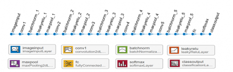
Figure 3. Architecture of the designed LWCNN
In the second step of our proposed framework, a lightweight CNN (LWCNN) was designed to improve perform the feature extraction and BT classification with low numbers of parameters. LWCNN is an architecture that is designed to be computationally efficient and have a small memory footprint, making it well-suited for deployment on mobile devices and other resource-constrained platforms.
There are many different architectures for lightweight CNNs, but they typically involve a combination of several design techniques, such as a reduction in model size, spatial reduction, depth wise separable convolution, pruning and quantization.
The goal of these design techniques is to accomplish a good trade-off among model accuracy and computational efficiency, making it possible to run the network on resource-limited devices with minimal latency and power consumption.
In Figure 3, the architecture of LWCNN is shown. It includes five convolutional blocks, each block contains a batch normalization layer, max-pooling layer and Leaky ReLU layer. The details of LWCNN are presented in Table 1.
Table 1. Details of the proposed LWCNN model
|
Name of layer |
Decimation |
# Of Filter |
Padding |
Stride |
|
Input |
224 224 3 |
|
|
|
|
Conv1 |
3 3 |
8 |
Same |
|
|
batch normalization |
|
|
|
|
|
leaky ReLU |
0.01 |
1 |
|
|
|
max-pooling |
2 2 |
|
|
2 2 |
|
Conv2 |
3 3 |
16 |
Same |
|
|
batch normalization |
|
|
|
|
|
leaky ReLU |
0.01 |
|
|
|
|
max-pooling |
2 2 |
|
|
2 2 |
|
Conv3 |
3 3 |
32 |
Same |
|
|
batch normalization |
|
|
|
|
|
leaky ReLU |
0.01 |
|
|
|
|
max-pooling |
2 2 |
|
|
2 2 |
|
Conv4 |
3 3 |
16 |
Same |
|
|
batch normalization |
|
|
|
|
|
leaky ReLU |
0.01 |
|
|
|
|
max-pooling |
2 2 |
|
|
2 2 |
|
Conv5 |
3 3 |
8 |
Same |
|
|
batch normalization |
|
|
|
|
|
leaky ReLU |
0.01 |
|
|
|
|
max-pooling |
2 2 |
|
|
2 2 |
|
Fully Connect |
4 |
|||
|
Softmax |
0 or 1 or 2 or 3 |
|||
|
Classification |
Glioma or meningioma or no_tumor or pituitary |
|||
LWCNN model is a kind of feed-forward neural network. The utilization of convolutions to capture translation invariance can significantly reduce the parameters numbers required, as the filter becomes independent of position. Convolutional, pooling, and fully linked layers make up the CNN model. These layers carry out a variety of tasks, including feature extraction, dimensionality reduction, and classification. In the convolution process of the forward pass, the filter slides over an input shape and computes a map of activation, which determines the point-wise value of every output [30].
The technique of batch normalization is employed to train deep neural networks effectively by normalizing the contributions to each layer for every mini-batch. In deep learning, constructing a neural network with multiple layers can be challenging due to the architecture of the learning algorithm and the underlying random weights in the initial setup. An underlying reason for this problem could be that resetting weights after each mini-batch can cause a shift in the distribution of inputs to the lower layers of the network, making the learning system continuously chase a moving target. The alteration in the input distribution to network layers caused by weight resetting is commonly known as internal covariate shift. The challenge arises from the fact that the model is updated layer-by-layer in reverse order, from the input to the output, while assuming that the weights in the preceding layers remain constant [31, 32].
To improve performance of deep neural networks, we incorporate batch normalization, which involves scaling the output of each layer. Recall that the term "normalization" refers to rescaling data so that the standard deviation and mean are both zero. The fixed input distributions that would eliminate the negative impacts of internal covariate shift might be achieved by brightening the inputs to individually layer. By normalizing the activations of the previous layer, the assumption that the following layer makes regarding the spread and distribution of inputs during weight update will remain relatively constant, if not entirely unchanged. The differences in the normalized inputs between training and inference might result in observable differences in performance for smaller mini-batches that don't contain an appropriate distribution of models from the training dataset. To address this issue, a modification to the existing technique called Batch Renormalization has been developed. It aims to stabilize the estimates across mini-batches of the variable mean and standard deviation.
Additionally, the benefits of batch normalization include: (a) Hyperparameter tuning has less impact on the model due to the implementation of this technique; (b) smaller internal covariant shift; (c) decreasing the dependence of gradients on the parameters scale or underlying values; (d) At this juncture, weight initialization is marginally less crucial due to the application of this technique; and (e) dropout can be eliminated for regularization.
“ReLU” is one of the most common activation functions utilized in neural networks. Researchers often incorporate this technique between layers to introduce nonlinearity and better handle datasets that are more complex and nonlinear in nature. Figure 4 shows ReLU that can be stated as in Eq. (2):
$f(x, y)=\left\{\begin{array}{c}0.01 \ \forall\ \ x<0 \\ x \ \forall\ \ x>0\end{array}\right.$ (2)
Figure 4. ReLU
Despite its popularity, particularly on DNN, ReLU has certain drawbacks. ReLU is not continuously differentiable, to start. Gradient cannot be calculated at x=0. Although it is not a major issue, it has a little impact on training effectiveness. All values are reset to zero by ReLU. However, since gradient of zero is zero, neurons arriving at high negative values cannot recover from being trapped at 0, which might be advantageous for sparse input. Since the neuron effectively dies, the issue is referred to as the dying ReLU problem.
Figure 5. Leaky ReLU
As a result, the network can effectively cease learning and perform poorly. Even though input values are fed to the neural network, the sum of input to the traditional ReLU is always negative despite the weights being appropriately initialized to small random values and large weight updates. The problem is not entirely solved, but current advancements in the ReLU, like the leaky LReLU that enables a greater degree of nonlinearity, allowing for the inclusion of small negative values or facilitating the transition from positive to small negative values. The aim of using the Leaky LReLU is to address these issues into a ReLU function by providing a small negative gradient for negative inputs. Figure 5 and Eq. (3) demonstrate the LReLU and its derivative.
$f(x, y)=\left\{\begin{array}{c}0 \forall\ \ x<0 \\ a x \forall\ \ x>0\end{array}\right.$ (3)
where, alpha is a small constant, typically around 0.01. If pixel value at location (x, y) is positive, then the Leaky ReLU function returns the pixel value unchanged. However, if the pixel value is negative, the function returns alpha times the pixel value.
The effect of the Leaky ReLU function on the image at location (x, y) depends on the pixel value at that location. If pixel value is positive, the function has no effect and returns the pixel value unchanged. If the pixel value is negative, the function applies a small negative slope to the pixel value, which can help prevent the gradient from vanishing during backpropagation in a neural network.
Max pooling selects only the highest activation value, while average pooling downplays the activation by combining the non-highest activations. This issue was addressed by Santurkar et al. [33] who suggested a hybrid strategy that included average pooling and maximum pooling. Dropout [34] and Drop Connect [35] are two major influences on this strategy. Eq. (4) may be used to represent mixed pooling.
$s j=\lambda \max a i+(1-\lambda) \frac{1}{R j} \sum_{i \in R j} a i$ (4)
The selection between max pooling and average pooling is determined by the value of $\lambda$, which is randomly assigned either a value of 0 or 1. If $\lambda$=0, the operation functions as average pooling, and if $\lambda$=1, it functions as max pooling. The value of $\lambda$ is saved for the forward-propagation phase and is utilized during the backpropagation process.
4.1 Dataset
Dataset used to evaluate our proposed method was acquired from Kaggle [36]. This dataset is a combination of the following from three datasets; figshare, SARTAJ and Br35H datasets. It’s about 3160 images in the whole dataset, which are divided into a training dataset (80%) and a testing (20%). The numbers of images in the two sets are 2528 and 623, respectively. The numbers of images from the four classes in the training and testing sets are summarized in Table 2.
Table 2. Characteristics of the dataset [36]
|
Types |
Training |
Testing |
Sum |
|
glioma meningioma no tumor pituitary |
741 750 317 721 |
185 187 79 180 |
926 937 396 901 |
|
Sum |
|
|
3160 |
The usage of the dataset was illustrated in Figure 6. The images were first pre-processed by resizing the original size to256×256×3 to reduce the input dimension of the designed LWCNN therefore the number of parameters of LWCNN and yield a lightweight CNN for this study. Subsequently, the MRI images were enhanced with the image enhancement technique [28]. Then the designed LWCNN was trained on pre-processed images in the training set.
Figure 6. Illustration of the use of the BT dataset
4.2 Model training and evaluation metrics
The LWCNN was implemented with MATLAB 2021a and trained on Windows 10 OS with 16 GB RAM, an AMD Ryzen 5 3550H CPU, and GFX 2.10 GHz. The max iterations and batch size were set to 790 and 32, respectively. Our model trained for 10 epochs which every epoch contains 79 iterations that walk throughout the whole training set.
The performance measurements employed in this work include accuracy, sensitivity, specificity, and precision [37, 38], which are the most often used metrics and are stated as follows in Eqns. (5)-(9):
Accurac $=\frac{T N+T P}{T P+F P+T N+F N}$ (5)
Sensitivity $=\frac{T P}{T P+F N}$ (6)
Specificity $=\frac{T N}{T N+F P}$ (7)
Precision $=\frac{T P}{T P+F P}$ (8)
$F_{\text {measure }}=\frac{2(\text { precision } * \text { sensitivity })}{\text { precision }+ \text { sensitivity }}$ (9)
4.3 Experiment results
The trained LWCNN was evaluated on the testing set. To demonstrate the effectiveness of the image, enhancement step in our proposed framework, we also generate results with the same pipeline except for disabling the enhanced process for comparison. The results related to these two settings are shown in Tables 3 and 4, respectively.
Table 3. Testing results of our proposed framework
|
Fm% |
Spe% |
Sen% |
Pre% |
Ac% |
Class |
|
92 91 93 99 |
94 98 99 99 |
97 87 91 100 |
87 95 96 98 |
95 95 98 99 |
glioma meningioma no_tumor pituitary |
Table 4. Testing results without image enhancement
|
Fm% |
Spe% |
Sen% |
Pre% |
Ac% |
Class |
|
88 84 84 95 |
94 95 98 96 |
89 81 80 100 |
86 88 89 91 |
92 91 96 97 |
glioma meningioma no_tumor pituitary |
Note: Ac=Accuracy, Pre=Precision, Sen=Sensitivity, Spe=Specificity Fm=F-measure.
It can be concluded from Table 3, that our approach can achieve accurate BTs classification performances in terms of accuracy, precision, sensitivity, specificity and F-measure for all four classes. Specifically, the F-measure for the four classes is 92%, 91%, 93%, and 99%, respectively. In addition, compared to the pipeline without an image enhancement process, the proposed method shows much better performance. Specifically, without the image enhancement step, the F-measure scores of the proposed approach drop by 88%, 84%, 84%, and 95%, respectively. This proves that image enhancement is critical for improving the prediction performance of the model.
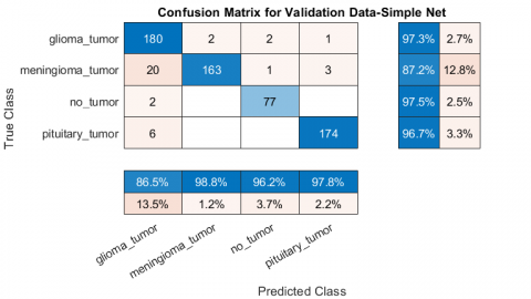
Figure 7. Confusion matrix related to testing results with image enhancement
Figure 8. Confusion matrix without image enhancement
To further validate the methods, we analyze the confusion matrices related to the testing results. The confusion matrices related to the setting with image enhancement and that without image enhancement are shown in Figures 7 and 8 respectively.
By comparing the Figures 7 and 8, we can see that with the image enhancement, our approach is able to make predictions that cause less confusion across different classes. This further validates the effectiveness of the enhancement in the pipeline.
Finally, to investigate the reason for the performance improvement caused by image enhancement step, we plot the accuracy and loss curves in the model training process for the two settings. The curves for the two settings were shown in Figures 9 and 10.
Figure 9. Accuracy and loss curves for the setting with image enhancement
Figure 10. The accuracy and loss curves for the setting without image enhancement
It can be observed in Figures 9 and 10 that training and validation accuracy curves are much closer in Figure 9 than those in Figure 10. The same trends can be observed on the loss curves in the two figures. These results show that image enhancement process is able to align the distributions of image samples in the training dataset and in the validation (testing) set, therefore greatly improving the performance of a deep learning model trained on a training set, when applied on a testing set. This proved that image enhancement is an important process for training our LWCNN model on the BT dataset.
We evaluated the performance of our proposed WLCNN method against state-of-the-art techniques in the literature. The comparative analysis revealed that the hybrid WLCNN approach outperformed these methods, demonstrating its superior efficiency as depicted in Table 5.
Table 5. The comparative results
|
Ac. |
Method |
year |
Ref |
|
95.23 92.98 84.00 96.00 95.86 96.75 |
GWO+M-SVM CNN CNN CNN CNN LWCNN |
2016 2018 2018 2019 2022 ---- |
[10] [24] [26] [7] [25] PM |
In this study, we presented framework based on deep learning for fully automatic BT classification with weighted enhanced MRI images. The proposed framework includes an image enhancement step for MRI quality improvement and a lightweight convolutional neural network (LWCNN). We evaluated our proposed method using a publicly accessible set of MRI brain images. It shows accurate classification performances in terms of accuracy, precision, sensitivity, specificity, and F-measure. This demonstrate that the proposed approach holds great promise to be applied in clinical applications. In addition, our studies show that an image enhancement process is helpful for training a deep learning model for BT classification since it allows homogenizing of samples distribution from the training set and from the testing set.
This work is supported by Princess Nourah bint Abdulrahman University Researchers Supporting Project number (PNURSP2023R193), Princess Nourah bint Abdulrahman University, Riyadh, Saudi Arabia.
[1] Ries, L.A.G., Smith, M.A., Gurney, J.G., Linet, M., Tamra, T., Young, J.L., Bunin, G.R. (1999). Cancer incidence and survival among children and adolescents: United states SEER program 1975-1995. National Cancer Institute, SEER Program. NIH Pub. No. 99-4649. Bethesda, MD.
[2] Brodeur, G.M., Maris, J.M. (2002). Neuroblastoma in Principles and practice of pediatric Oncology. Pizzo PA and Poplack DG.
[3] Radcliffe, J., Packer, R.J., Atkins, T.E., Bunin, G.R., Schut, L., Goldwein, J.W., Sutton, L.N. (1992). Three-and four-year cognitive outcome in children with noncortical brain tumors treated with whole‐brain radiotherapy. Annals of Neurology: Official Journal of the American Neurological Association and the Child Neurology Society, 32(4): 551-554. https://doi.org/10.1002/ana.410320411
[4] Pradhan, A., Mishra, D., Das, K., Panda, G., Kumar, S., Zymbler, M. (2021). On the classification of MR images using “ELM-SSA” coated hybrid model. Mathematics, 9(17): 2095. https://doi.org/10.3390/math9172095
[5] Byrne, J., Dwivedi, R., Minks, D. (2014). Recommendations Cross sectional imaging cancer management. 2nd ed., Royal College of Radiologists: London, UK, pp. 1-20.
[6] Afshar, P., Plataniotis, K.N., Mohammadi, A. (2019). Capsule networks for brain tumor classification based on MRI images and coarse tumor boundaries. In ICASSP 2019-2019 IEEE International Conference on Acoustics, Speech and Signal Processing (ICASSP), pp. 1368-1372. https://doi.org/10.1109/ICASSP.2019.8683759
[7] Sultan, H.H., Salem, N.M., Al-Atabany, W. (2019). Multi-classification of brain tumor images using deep neural network. IEEE Access, 7: 69215-69225. https://doi.org/10.1109/ACCESS.2019.2919122
[8] Louis, D.N., Perry, A., Reifenberger, G., Von Deimling, A., Figarella-Branger, D., Cavenee, W.K., Ohgaki, H., Wiestler, O.D., Kleihues, P., Ellison, D.W. (2016). The 2016 World Health Organization classification of tumors of the central nervous system: A summary. Acta Neuropathologica, 131(6): 803-820. https://doi.org/10.1007/s00401-016-1545-1
[9] Hsieh, K.L.C., Lo, C.M., Hsiao, C.J. (2017). Computer-aided grading of gliomas based on local and global MRI features. Computer Methods and Programs in Biomedicine, 139: 31-38. https://doi.org/10.1016/j.cmpb.2016.10.021
[10] Sachdeva, J., Kumar, V., Gupta, I., Khandelwal, N., Ahuja, C.K. (2016). A package-SFERCB- “Segmentation, feature extraction, reduction and classification analysis by both SVM and ANN for brain tumors”. Applied Soft Computing, 47: 151-167. https://doi.org/10.1016/j.asoc.2016.05.020
[11] Raja, S.S. (2019). Deep learning based image classification and abnormalities analysis of MRI brain images. In 2019 TEQIP III Sponsored International Conference on Microwave Integrated Circuits, Photonics and Wireless Networks (IMICPW), pp. 427-431. https://doi.org/10.1109/IMICPW.2019.8933239
[12] Capra, M., Bussolino, B., Marchisio, A., Shafique, M., Masera, G., Martina, M. (2020). An updated survey of efficient hardware architectures for accelerating deep convolutional neural networks. Future Internet, 12(7): 113. https://doi.org/10.3390/fi12070113
[13] Yafooz, W.M., Alsaeedi, A., Alluhaibi, R., Abdel-Hamid, M.E. (2022). Enhancing multi-class web video categorization model using machine and deep learning approaches. International Journal of Electrical and Computer Engineering (IJECE), 12(3): 3176. http://doi.org/10.11591/ijece.v12i3.pp3176-3191
[14] Hu, M., Zhong, Y., Xie, S., Lv, H., Lv, Z. (2021). Fuzzy system based medical image processing for brain disease prediction. Frontiers in Neuroscience, 15: 714318. https://doi.org/10.3389/fnins.2021.714318
[15] Maqsood, S., Damasevicius, R., Shah, F.M. (2021). An efficient approach for the detection of brain tumor using fuzzy logic and U-NET CNN classification. In Computational Science and Its Applications–ICCSA 2021: 21st International Conference, Cagliari, Italy, September 13–16, 2021, Proceedings, Part V 21, pp. 105-118. https://doi.org/10.1007/978-3-030-86976-2_8
[16] Raza, A., Ayub, H., Khan, J.A., Ahmad, I., Salama, A.S., Daradkeh, Y.I., Javeed, D., Ur Rehman, A., Hamam, H. (2022). A hybrid deep learning-based approach for brain tumor classification. Electronics, 11(7): 1146. https://doi.org/10.3390/electronics11071146
[17] Kadry, S., Damaševičius, R., Taniar, D., Rajinikanth, V., Lawal, I.A. (2021). U-net supported segmentation of ischemic-stroke-lesion from brain MRI slices. In 2021 Seventh International conference on Bio Signals, Images, and Instrumentation (ICBSII), pp. 1-5. https://doi.org/10.1109/icbsii51839.2021.9445126
[18] Leo, M.J. (2019). MRI brain image segmentation and detection using K-NN classification. In Journal of Physics: Conference Series, 1362(1): 012073. https://doi.org/10.1088/1742-6596/1362/1/012073/meta
[19] Farhi, L., Zia, R., Ali, Z.A. (2018). Performance analysis of machine learning classifiers for brain tumor MR images. Sir Syed University Research Journal of Engineering & Technology, 8(1): 6-6. https://doi.org/10.33317/ssurj.v8i1.36
[20] Veeraraghavan, A.K., Roy-Chowdhury, A., Chellappa, R. (2005). Matching shape sequences in video with applications in human movement analysis. IEEE Transactions on Pattern Analysis and Machine Intelligence, 27(12): 1896–1909. https://doi.org/10.1109/TPAMI.2005.246
[21] Mohsen, H., El-Dahshan, E.S.A., El-Horbaty, E.S.M., Salem, A.B.M. (2018). Classification using deep learning neural networks for brain tumors. Future Computing and Informatics Journal, 3(1): 68-71. https://doi.org/10.1016/j.fcij.2017.12.001
[22] Litjens, G., Kooi, T., Bejnordi, B.E., Setio, A.A.A., Ciompi, F., Ghafoorian, M., Van der Laak, J., Van Ginneken, B., Sánchez, C.I. (2017). A survey on deep learning in medical image analysis. Medical Image Analysis, 42: 60-88. https://doi.org/10.1016/j.media.2017.07.005
[23] Akkus, Z., Galimzianova, A., Hoogi, A., Rubin, D.L., Erickson, B.J. (2017). Deep learning for brain MRI segmentation: state of the art and future directions. Journal of Digital Imaging, 30: 449-459. https://doi.org/10.1007/s10278-017-9983-4
[24] Nazir, M., Shakil, S., Khurshid, K. (2021). Role of deep learning in brain tumor detection and classification (2015 to 2020): A review. Computerized Medical Imaging and Graphics, 91: 101940. https://doi.org/10.1016/j.compmedimag.2021.101940
[25] Pereira, S., Meier, R., Alves, V., Reyes, M., Silva, C.A. (2018). Automatic brain tumor grading from MRI data using convolutional neural networks and quality assessment. In Understanding and Interpreting Machine Learning in Medical Image Computing Applications: First International Workshops, MLCN 2018, DLF 2018, and iMIMIC 2018, Held in Conjunction with MICCAI 2018, Granada, Spain, September 16-20, 2018, Proceedings 1, pp. 106-114. https://doi.org/10.1007/978-3-030-02628-8_12
[26] Abiwinanda, N., Hanif, M., Hesaputra, S.T., Handayani, A., Mengko, T.R. (2019). Brain tumor classification using convolutional neural network. In World Congress on Medical Physics and Biomedical Engineering 2018: June 3-8, 2018, Prague, Czech Republic (Vol. 1), pp. 183-189. https://doi.org/10.1007/978-981-10-9035-6_33
[27] Saad, A. (2022). New datasets- Brain Tumors MRI Images (figshare, SARTAJ and Br35H). figshare. https://doi.org/10.6084/m9.figshare.21325758
[28] Saad, A., Kamil, I.S., Alsayat, A., Elaraby, A. (2022). Classification COVID-19 based on enhancement X-Ray images and low complexity model. Computers, Materials and Continua, 72(1): 561-576.
[29] Al-Ameen, Z., Muttar, A., Al-Badrani, G. (2019). Improving the sharpness of digital image using an amended unsharp mask filter. International Journal of Image, Graphics & Signal Processing, 11(3): 1-9. https://doi.org/10.5815/ijigsp.2019.03.01
[30] Xiong, J., Yu, D., Wang, Q., Shu, L., Cen, J., Liang, Q., Chen, H.Y., Sun, B. (2021). Application of histogram equalization for image enhancement in corrosion areas. Shock and Vibration, 2021: 1-13. https://doi.org/10.1155/2021/8883571
[31] Zhang, S., Yao, L., Sun, A., Tay, Y. (2019). Deep learning based recommender system: A survey and new perspectives. ACM Computing Surveys (CSUR), 52(1): 1-38. https://doi.org/10.1145/3285029
[32] Ioffe, S., Szegedy, C. (2015). Batch normalization: Accelerating deep network training by reducing internal covariate shift. In International conference on machine learning, pp. 448-456.
[33] Santurkar, S., Tsipras, D., Ilyas, A., Madry, A. (2018). How does batch normalization help optimization?. Advances in Neural Information Processing Systems, 31.
[34] Yu, D., Wang, H., Chen, P., Wei, Z. (2014). Mixed pooling for convolutional neural networks. In Rough Sets and Knowledge Technology: 9th International Conference, RSKT 2014, Shanghai, China, October 24-26, 2014, Proceedings 9, pp. 364-375. https://doi.org/10.1007/978-3-319-11740-9_34
[35] Hinton, G.E., Srivastava, N., Krizhevsky, A., Sutskever, I., Salakhutdinov, R.R. (2012). Improving neural networks by preventing co-adaptation of feature detectors. arXiv preprint arXiv:1207.0580. https://arxiv.org/abs/1207.0580
[36] Msoud Nickparvar. (2021). Brain tumor MRI dataset, [Data set]. Kaggle. https://doi.org/10.34740/KAGGLE/DSV/2645886.
[37] Powers, D.M. (2020). Evaluation: from precision, recall and F-measure to ROC, informedness, markedness and correlation. arXiv preprint arXiv:2010.16061. https://arxiv.org/abs/2010.16061
[38] Davis, J., Goadrich, M. (2006). The relationship between Precision-Recall and ROC curves. In Proceedings of the 23rd International Conference on Machine Learning, pp. 233-240. https://doi.org/10.1145/1143844.1143874