Varsha P. Gaikwad*![]() | Vijaya Musande
| Vijaya Musande![]()
© 2023 IIETA. This article is published by IIETA and is licensed under the CC BY 4.0 license (http://creativecommons.org/licenses/by/4.0/).
OPEN ACCESS
Crop leaf diseases have a significant impact on a country's agricultural economy, as crop yield is essential for promoting economic growth. Manual detection of these diseases is time-consuming and inefficient. Consequently, researchers have developed various techniques for the automated detection of plant diseases. In this study, we propose a novel approach to identify crop diseases using a deep k-Nearest Neighbors (KNN) classifier optimized via Cetalatran optimization. Cetalatran optimization rapidly identifies the most relevant features for disease prediction, allowing for early and efficient detection. The performance of the Cetalatran-optimized deep k-NN algorithm is evaluated using accuracy, sensitivity, and specificity metrics. The proposed method yields improved results, with accuracy, sensitivity, and specificity values of 91.879%, 92.736%, and 95.951%, respectively, demonstrating its superior efficiency compared to existing techniques.
crop leaf disease, cetalatran optimization, economy, deep KNN classifier, parameter metrics
Agriculture plays a crucial role in determining a country's economy. Thus, it is vital to educate farmers about leaf diseases and the application of technology for disease identification. Globally, crop infections significantly impact crop yields, reducing the average annual soybean yields in the United States by 11% [1]. Between 2010 and 2014, crop diseases in soybean led to estimated economic losses of $23 billion in the US and Canada [2]. Detecting and controlling crop diseases requires considerable effort, and the introduction of disease-tolerant crop varieties is necessary to improve economic significance. However, current scouting and phenotyping techniques for disease prediction rely on human scouts and visual assessments, which are subject to human error, individual biases, and inter- and intra-rater variability [3-6]. To enhance yield protection through mitigation strategies, novel technologies for disease detection and identification beyond visual evaluations are required.
Various symptoms of infection include reddish-brown lesions on seedling hypocotyls, which often remain invisible until later developmental stages, R5-R7. Other symptoms comprise reddish-brown discoloration of vascular tissue, chlorosis, wilting, and early senescence of plants with leaves and petioles still attached [7-10]. Computer vision has been widely employed to enhance grain yield as a precision agriculture tool [11]. Prompt and accurate identification of plant pathogens is essential for applying timely disease management strategies [12, 13]. Plant scouting for disease detection is a critical component of Integrated Pest Management. However, visual scouting is time-consuming, expensive, and demands a certain level of pest identification expertise, making disease diagnosis findings potentially subjective [14-29]. Early and accurate disease diagnosis is crucial for selecting effective active components in spray treatments and minimizing the quantity needed, which has significant environmental and economic implications.
Various methods relying on Unmanned Aerial Vehicles (UAV) have been introduced for crop phenotyping and infection diagnoses. Artificial intelligence and machine learning are commonly used models [15], with a UAV-based high-throughput phenotyping system developed for citrus crop analysis. This automated system accurately predicts and analyzes tree count and gap, individual health status, and canopy size using the normalized difference vegetation index [30]. Convolutional neural networks (CNN) have gained popularity due to their impressive classification results in images with varying complexities. Several CNN-based methods [16] have been employed to differentiate disease-affected images belonging to multiple plant species, with images captured under controlled conditions. However, the processing of deep neural networks [18] often avoids laboratory-collected samples, using input images gathered under authentic field conditions with varying object sizes, lighting, and scenery changes to predict nine types of infectious diseases and pests in tomato plants among 25 different plant species [19, 31].
The primary objective of this research is to determine the presence of leaf diseases in individuals with high efficiency. Initially, data are collected from a multispectral image database, and the concatenation of vegetation indices with the original image is performed in the preprocessing stage. After concatenation, the most relevant and informative features are selected based on the Relief algorithm and are then subjected to the deep k-NN classifier. The training and testing of data are carried out using the deep k-NN classifier, which effectively classifies the presence of diseases in plants using multispectral images. The deep k-NN classifier is optimally tuned using Cetalatran optimization to achieve the best solution within an optimal time frame. The main contributions of this research include:
The remainder of this paper is organized as follows: Section 2 reviews existing works on leaf disease classification and discusses their advantages and disadvantages. Section 3 details the Cetalatran optimization algorithm, its procedure, and functioning. Section 4 elucidates the disease prediction model for detecting crop diseases. Section 5 provides a comprehensive description of the results, and Section 6 concludes the study.
Detecting the plant disease helps the farmers to get rid of the economical loss and that leads to the improvement of the country's economical growth and people's nutritional growth. Plant disease technologies should be improved with the overcome of the limitations. An efficient classifier is essential for the accurate prediction of plant disease and the classifiers performance can be improved with the involvement of an optimizer to find the optimal solution in leaf disease prediction.
In the following section, the previous works undertaken by various researchers along with the advantages and disadvantages are described.
2.1 Literature review
The various works undertaken in the crop disease classification are enumerated as follows: Koushik Nagasubramanian et al. [7] introduced a 3D deep convolutional neural network that utilized a pretrained model for the classification of diseases but the classification is performed using a small dataset. Similarly, Abdulridha et al. [30] initiated a Stepwise discriminate analysis that constructed the model through step by step process and a Multilayer perceptron but the drawback is that this method is inaccurate and sometimes leads to misclassification. Chen et al. [31] introduced an economically advanced, reduced sampling method that reduced the complexities aroused in collecting the data yet; it has a lesser probability in choosing true representative samples. Tetila et al. [11] established a clustering mechanism relying on simple linear iterative clustering that had the capability to recognize the boundary as well as it has strong robustness. Performing the steps separately and updating in convergence rate increases the time complexity. Abdulridha et al. [32] progressed a radial basis function that has a strong learning capacity as well it is less vulnerable to noise, nevertheless, it assigns the same weight to all the attributes. Hu et al. [33] introduced a deep learning method that detected the features automatically without human intervention and the classifier is optimally tuned on the desired outcome but there is a necessity for a large amount of data. Yu et al. [34] developed a hyperspectral method that maintained a spectral relationship between the spectra, especially with neighborhood spectrums but this method needs a detailed description of images. Bhandari et al. [35] developed a Small Unmanned Aerial Vehicle that provided overall access to the places where it is difficult to reach but it causes damage to people and humans.
The multi-spectral image database has multiple layers of images that are separated on vegetation indices that resolve the time complexity. The conventional optimizers that were present assign the same weight whereas the cetalatran optimization effectively adjusts the weights that provide the optimal solution hence the time complexity is reduced and the convergence rate is improved.
2.2 Challenges
The following are the challenges needed to overcome:
The cetalatran optimization algorithm is formed by the standard hybridization of the DSO [20] and COA [21] optimization algorithms. The cetacean has the capability to identify the prey by producing click sounds and the canis latrans has the power to communicate effectively with other canis latrans the best adaptable canis latran is selected as the best solution. Coagulating the characteristics of the cetacean and canis latrans, the location of the prey is identified using the cetatcean technique, and the best fittest prey is determined using the latrans techniques. The resultant is the fittest prey along with its position.
3.1 Motivation
The cetacean refers to the family Delphinidae and is around 1.7m long. The cetacean has the capability to travel under the speed of 29 kilometers per hour and the prey that moves very fast are captured using the canonical teeth the hearing capacity of the cetacean is good in both air and water. Similarly, canis latrans belong to the family canine and they live as a pack where socialization and communicative behavior are performed effectively. The best individuals that adapt well to the environment are selected as the leader.
3.2 Mathematical model for the cetalatran optimization algorithm
The cetacean has the capability to initiate a click sound for communication, which differs from other animals in their communicative behavior [25]. The released click sound strikes the target object or prey and some amount of energy is projected back to the cetacean. As soon as the signal is received, the cetacean immediately transmits another click sound for the evaluation of the distance between the target prey, the direction of the target present. The echoes reflected from the target are received at the head of the dolphin at both ends, which is helpful in determining the direction of the location of the prey. The cetacean incessantly transmits the click and receives the echoes, which helps in tracking of the target prey. The clicks made by the cetacean are directional and are echolocate that frequently occurring as an object of interest.
3.2.1 Foraging phase
The foraging of prey using the technique of echolocating is considered as the foundation of optimal solutions for the problems. The cetacean concentrates mainly on the location of the prey, which can be identified by the behavior of identification of the target and once the target is reached it stops foraging and starts sending more clicks to focus on the prey. The foraging characteristics of the cetacean are limited when the prey is spotted and the reduction of the exploration takes place hence the foraging is proportional to the distance of the position of the prey. The cetacean targets the prey relying upon two aspects, such as initially the global search is carried out by searching all the places inclusively comes under the first aspect and the results obtained in the previous stage is concentrated in the second aspect. These are some of the most intrinsic characteristics present in most meta-heuristic algorithms. The ratio between the first and second aspects, from the random values, is generated using the convergence factor [22]. Relying upon a predefined curve the user has the capability to vary the ratio extracted from aspects 1 and 2 which helps to control the search depending on the needs that is the searches can be converted from global to local on the user individually.
3.2.2 Boundary phase
Initially, the searching space of the cetacean should be sorted depending on the rules mentioned below.
Ordering of boundary phase: In the beginning, the optimization of one and all variables takes place by deriving all the possible solutions in the search space and at the same time the solutions are arranged in an ascending or descending order. If the occurrence of more than one characteristic variable occurs then the sorting is performed on the significant characteristic variable. In the cetacean optimization, the vector variable $D C_k$ is initiated and here, D represents the length of the vector $C_k$ and k is the variable that helps in assigning the vectors to particular order as a matrix column. The matrix solution $S_{m * n}$ is initiated where the factor m represents the maximum value of the vector given by, $\left(D C_k\right)_{k=1: n}$ and $n$ represents the number of variables.
The variation in the curve during the process of optimization solely relies on the convergence factor which is predefined. Change of the convergence factor relying upon the curve is given by:
$F(L)=Z+\left(1-Z \frac{\left(L_k^p-1\right)}{\left(Z_n\right)^p-1}\right)$ (1)
where, F is the fixed probability that is predefined, Z is the convergence factor in the first iteration L plays a main contribution in reducing the expensive, where the solutions are fixed in a random manner and $L_k$ is the number of iterations that takes place and n represents the number of loop. The degree of the curve is represented by $p$ and $k$ is the fitness function assigned here for attaining the best solution.
3.2.3 Interacting phase
The canis latrans lives in group and depending on the population they are categorized into two classes where in the first class, the population of canis latrans remains constant hence the solitary canis latrans are not taken into account for the simplified view and other than these every canis latrans are assigned as a possible solution. The social condition of the canis latrans are the objective function. The important characteristics of the canis latrans are the flexibility to adapt to the environment and the exchanging of information in an effective way. There are around 14 coyotes present in a single pack and when the interchanging of the individuals occurs in the group the information also gets exchanged, represented by the following equation,
${{G}^{h,t}}=\left\{ \operatorname{com}_{g}^{h,t}\left| {{\arg }_{\left. {{g}_{-\left\{ 1,2,3,\ldots .{{J}_{f}} \right\}}} \right\}}}\quad\quad \right|\min f\left( \operatorname{com}_{g}^{h,t} \right) \right\}$ (2)
where, G is the canis latran that adapted well to the environment, and com denotes the social-communicative behavior of the canis latrans present in the pack h in the time instant t. g is the individual canis latrans present in the pack and when the best individuals are selected the best solution is obtained.
3.2.4 Renovating phase
When the strategy of selecting the best solution from the canis latrans is combined with the foraging characteristics of cetacean, the finest and fittest prey is selected depending on the information gained through the communication behavior of the canis latrans. This reduces the number of iterations takes place and the time consumed in optimizing features is also reduced due to the understanding of the characteristics.
$F_{n e w}(L)=G^{h, t}\left\{Z+\left(1-Z \frac{\left(L_k^p-1\right)}{\left(Z_n\right)^p-1}\right)\right\}$ (3)
where, $F_{n e w}$ denotes the new finest solution and $G^{h, t}$ is the best candidate solution obtained from the canis latrans and when it gets coagulated with the probability of getting the prey in a predefined manner, the probability is converted to a stability factor of getting the best and finest suitable solution which improves the efficiency of the model. The algorithmic procedure of the cetalatran optimization algorithm is enumerated in Table 1.
Table 1. Algorithm: Pseudocode for the cetalatran optimization
|
Pseudo code for the proposed Ceta-latrans optimization |
|
|
|
|
|
|
|
|
|
|
|
|
|
|
|
|
|
|
|
|
|
|
|
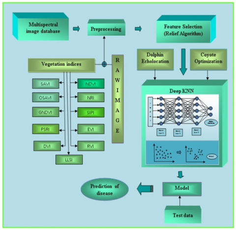
The main intention of the research is to determine the disease in crops by availing the deep KNN classifier utilizing high-resolution hyperspectral UV images. The images are collected from the multispectral image dataset and are fed to the preprocessing stage in order to enhance the functioning of the image by avoiding the distortions or noise present in the image. In the preprocessing stage, the original image is concatenated along with the vegetation. After the preprocessing stage, the important features from the images that are relevant to the crop disease prediction are selected using the relief algorithm. Then the selected features are trained using the deep KNN classifier using the high-resolution image and the deep KNN classifier is optimally tuned using the cetalatran optimization algorithm that is obtained from Dolphin Ecolocation and coyote optimization. The dolphins are experts in locating the prey using sound waves and the coyotes that live in groups are highly capable of communicating with each other during the hunting process. These behaviors are obtained mathematically, with four phases that are the foraging phase, boundary phase, interacting phase, and renovating phase that helps to reduce the losses and prevents the expenses by tuning the internal parameters. Finally, the presence of the diseases is evaluated using the deep KNN classifier. Figure 1 shows the representation of the crop disease prediction model using the deep KNN classifier.
Figure 1. Block diagram for the prediction of crop diseases
4.1 Input for the crop disease prediction model
In the beginning, the input from the multispectral image database [24] is taken into account for the effective detection of the disease present in the crop leaves and is given by,
$A=\left\{H_{1,2 \ldots \ldots \ldots . . q}\quad\right\}$ (4)
where, A is the set that consists of the multispectral images and H represents the individual multispectral image the number of input images ranges from [1, q].
4.2 Preprocessing
The preprocessing stage involves the enhancement of the input through the concatenation of vegetation indices. The processing of the information with respect to the color bands present in the multispectral images are evaluated for gaining information about the vegetation present in the captured image.
4.2.1 Vegetation indices
The enhancement of the information about the vegetation through the spectral transformation is carried through the vegetation index and there are around twenty-seven vegetation indices and in our research the indices, such as Normalized Difference Vegetation Index (NDVI), Soil Adjusted Vegetation Index (SAVI), Optimized Soil Adjusted Vegetation Index (OSAVI) nitrogen reflectance index (NRI), Green normalized difference vegetation index (GNDVI), Structure intensive pigment index (SIPI), Plant senescence reflectance index (PSRI), Enhanced vegetation index (EVI), Difference vegetation index (DVI), Ratio vegetation index (RVI), light leaf spot index (LLSI).
NDVI index: The NDVI helps to identify the variation between the natural as well as artificial land covers along with that the state of the vegetation is also determined using the NDVI. The vegetated areas could be identified and visualized in the maps using NDVI. The index NDVI is a dimensionless index and the working of this index is on determining the variation between the visible and near-infrared reflectance. The intensity of the green vegetation in the land cover is measured using this index. The NDVI index is measured by calculating the difference between the near-infrared and the red reflectance to the sum of the two rays given by
$N D V I_t=\frac{R_{\text {near-infinf } r \text { ared }}\quad\quad-R_{\text {red }}}{R_{\text {near-infinf } r \text { ared }}\quad\quad+R_{\text {red }}}$ (5)
where, the factor t represents the NDVI observed at a particular interval of time and the observed values is in the range of -1 and 1 where the lowest value represents the lack of density in the green vegetation and the highest value represents the healthy or high-density vegetation. The drought in the vegetation can also be monitored using the NDVI index.
SAVI index: The SAVI index is used for minimizing the influence of brightness in the image. The brightness of the soil is minimized using the SAVI index utilizing a soil brightness correction factor. The SAVI index is calculated and is given by
$S A V I=\frac{R_{\text {near-infinf } r \text { ared }}}{R_{\text {red }}} \quad\times(1+G)$ (6)
where, $R_{\text {infinf } r \text { ared }}$ is the pixel in the image near to the infrared band and $R_{\text {red }}$ is the pixel present in the image near the red band and G is the total amount of the vegetation in the land cover. The value of G varies relies upon the vegetation cover and when $G=1$, there is no green vegetation, and when $G=0.5$ then there is moderate green vegetation, and when the value of $G=0$ then the area consists of a high amount of green vegetation.
OSAVI index: The OSAVI index is used for the purpose of initiating a suitable background by adjusting the background parameters and is given by
$O S A V I=1.16 * \frac{R_{\text {near-infinf rared }}\quad\quad-R_{\text {red }}}{R_{\text {near-infinf } r \text { ared }}\quad\quad+R_{\text {red }}+R_{C F}}$ (7)
where, $R_{C F}$ is the calibration factor that consists of the value of 0.16 and it helps in determining the threshold values.
NRI index: The amount of nitrogen present in the vegetation is identified using the NRI index and is given by
$N R I=\frac{R_{\text {green }}\quad-R_{\text {red }}}{R_{\text {green }}\quad+R_{\text {red }}}$ (8)
GNDVI index: The photosynthetic activity of the vegetation is determined using the GNDVI index and it also provides information about the quantity of water and the nitrogen contents present in the vegetation and is determined using the formula,
$G N D V I=\frac{R_{\text {near-infinf r ared }}\quad\quad-R_{\text {green }}}{R_{\text {near-infinf r ared }}\quad\quad+R_{\text {green }}}$ (9)
SIPI index: The SIPI index is used for monitoring purposes that provides information about the health condition of the vegetation along with the physiological stress factor and the yield of the crop is also identified using the SIPI index. The increased value of the SIPI index shows that the plant is affected by the canopy stress pigment and is given by the formula,
$S I P I=\frac{R_{\text {near-infinf } r \text { ared }}\quad\quad-R_{\text {blue }}}{R_{\text {near-infinf } r \text { ared }}\quad\quad+R_{\text {blue }}}$ (10)
PSRI index: The carbon content of the cellulose and the lignin present in the dry state can be identified using the PSRI index and it also helps in analyzing the ignitability of the vegetation and is given by
$P S R I=\frac{R_{\text {red }}-R_{\text {blue }}}{R_{\text {near-infinf rared }}}$ (11)
EVI index: In highly biomass regions, the monitoring can be enhanced by the enhancement of the vegetation signal. The vegetation signal is improved by the degradation of atmospheric influences and decoupling of the canopy background signal and is given by
$E V I=2.5 * \frac{\left(R_{\text {near-infinf } r \text { ared }}\quad\quad-R_{\text {red }}\right)}{R_{\text {near-infinf r red }}\quad\quad+6 * R_{\text {red }}-7.5 * R_{\text {green }}+1}$ (12)
DVI index: The density of the green area present in the vegetation is determined by analyzing the difference between the visible and near-infrared reflectance, and the DVI is a dimensionless index and is determined using the formula,
$D V I=R_{\text {near-infinf } r \text { ared }}-R_{\text {red }}$ (13)
RVI index: The RVI index is utilized to differentiate the green leaves from other objects and is also used in determining the biomass of the captured image. The SR index is evaluated by estimating the ratio between the reflectance of near-infrared and red bands and is given by
$R V I=\frac{R_{\text {near-infinf } r \text { ared }}}{R_{\text {redbands }}}$ (14)
The green leaves always exhibit a minimized reflectance in the blue and red regions. The SR value for green is greater than 1 and for the other regions it assigns a value closer to 1.
LLSI index: In this research, the light leaf spot disease is particularly measured so that this index is availed for the effective utilization of the information. This index determines the area affected by the light leaf spot-affected tissue and is given by
$L L S I=\frac{R_{\text {red }}-R_{\text {green }}}{R_{\text {red }}+R_{\text {green }}}-R_{\text {infinf } r \text { ared }}$ (15)
4.3 Feature selection
The complexity of the input vectors are minimized by the feature selection techniques, where the more relevant and necessary features are selected for the proceedings. In this research, the features are selected through the relief algorithm due to high efficiency, and a brief description of the relief algorithm is enumerated below.
4.3.1 Relief algorithm
The relief algorithm helps to identify the more relevant features that are needed in the prediction of the presence of diseases in crop leaves by evaluating the strong dependencies and quality of attributes. Consider an instance that consists of a number of features spresent in the set $Q$ of size land the set of features is represented by $\left\{k_1, k_2, k_3 \ldots \ldots k_s\right\}$. A particular instance $Y$ from the set of s-dimensional vectors is given by $\left\{y_1, y_{2,} y_3 \ldots \ldots y_s\right\}$ and here $y_r$ represents the $k_r$ in the set $Y$.
The training data represented by $Q$ consists of the sample size $j$ and the threshold of the relevant feature selection is notified by $\varphi_{t h}$ and the value of the threshold ranges from $0 \leq$ $t \leq 1$. The feature is measured in the form of nominal or numerical that contains Boolean function, integer numbers or real values. When the values are nominal, the variation between the feature values $Y$ and $Z$ is given by the difference between the following function and the features given by:
$\operatorname{diff}\left(u_i, v_i\right)=\left\{0 ;\right.$ if $u_i=v_i 1 ;$ if $\left.u_i \neq v_i\right\}$ (16)
When the values are numerical, the variation between the feature values Y and Z is given by the difference between the following function and the features are given by
$\operatorname{diff}\left(u_i, v_i\right)=\frac{\left(u_i-v_i\right)}{N_i}$ (17)
where, N is the normalization unit that normalizes the variation in the values present in the interval [0, 1].
The relief algorithm selects the feature that consists of triad functions in the instance Y, near hit instance and near miss instance. The relief algorithm assigns weight to every feature present in the training dataset, and then the average of the weight of the features that are relevant to determine disease prediction in the crops are selected which is higher than the threshold $\varphi_{t h}$.
4.4 Deep KNN classifier for the prediction of crop disease
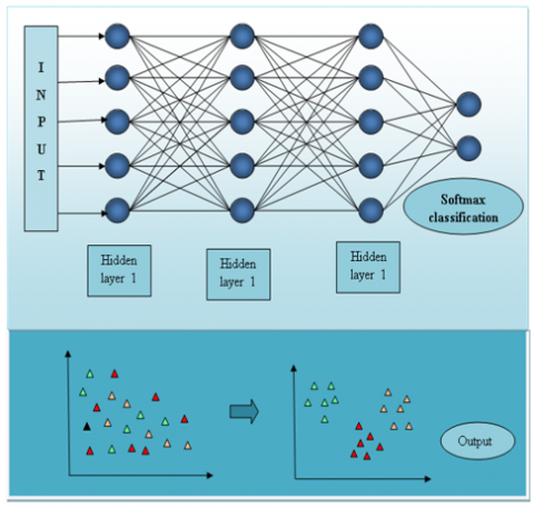
Figure 2. Architectural representation of the deep KNN classifier
The KNN classifier is employed here because of the characteristic of interpretation made with high accuracy in less period of time. In the classification of multi-class data, the deep KNN classifier classifies the data with more accuracy and reliability. The input applied to the KNN classifier is processed in the hidden layers and then the classification is performed in the softmax classification layers. The hidden layers are mathematical functions and every layer provides a specific output intended for the target of disease prediction. The predictions made by the model as well as the predictions made from the training data are evaluated and the relationship between the two predictions is explicated. The architectural representation of the deep KNN classifier is shown in Figure 2.
After performing the training of neural network $I$, the output produced by the layers is tracked and the output is represented by $I_\eta$, where $\eta \in 1 \ldots \ldots i$. For each layer $\eta$ present in the neural network, the layers are represented by the presence of training data associated with labels that help in determining the nearest neighbor, and the neighbors with similar characteristics are clustered for effective classification.
The results obtained for the crop leaf disease detection using the cetalatran-deep KNN, along with its supremacy are enumerated in the following section.
5.1 Experimental setup
The process of disease detection in the crop leaves is carried out using the software MATLAB in the windows 10 operating system using the Multispectral images of light leaf spot in the oilseed rape [28] dataset.
5.2 Dataset description
The dataset consists of normalized multispectral as well as photometric stereo images that consist of the images of plants as well as detached leaves. The dataset consists of the diseased image of a light leaf spot under the categories of 3D Imaging, Hyperspectral Imaging, Plant Disease Resistance, and Oilseed Crops.
5.3 Parameter metrics
The parameter metrics are used for the evaluation of the cetalatrans optimization-deep CNN and in this research, the accuracy, sensitivity, and specificity are measured.
Accuracy: The number of instances that are correctly identified by the cetalatran-deep KNN are given by:
$A c c=\frac{\text { True }_{p o s}+\text { True }_{n e g}}{\text { True }_{p o s}+\text { True }_{n e g}+\text { False }_{p o s}+\text { False }_{n e g}}$ (18)
Sensitivity: The actual positive values identified by the cetalatran optimization is given by sensitivity and is measured by:
Sens $=\frac{\text { True }_{\text {pos }}}{\text { True }_{\text {pos }}+\text { False }_{n e g}}$ (19)
Specificity: The number of non-diseased plant identified by the cetalatran optimization-deep CNN and is measured by:
Spec $=\frac{\text { True }_{n e g}}{\text { True }_{n e g}+\text { False }_{p o s}}$ (20)
5.4 Experimental results
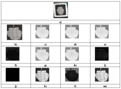
The multispectral image used for the detection of the plant leaf disease is shown in the input image and the various vegetation indexes are shown in Figure 3.
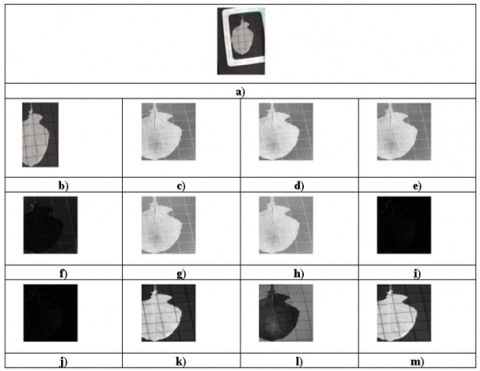
Figure 3. Experimental results of the cetalatran optimization-deep CNN method for sample 1 a) Input b) ROI c) NDVI d) SAVI e) OSAVI f) NRI g) GNDVI h) SIPI i) PSRI j) EVI k) DVI l) RVI m) LLSI
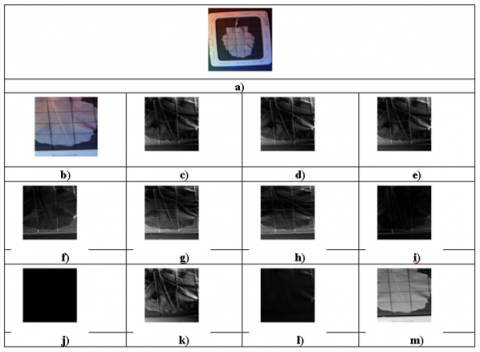
Figure 4. Experimental results of the cetalatran optimization-deep CNN method for sample 2 a) Input b) ROI c) NDVI d) SAVI e) OSAVI f) NRI g) GNDVI h) SIPI i) PSRI j) EVI k) DVI l) RVI m) LLSI
Figure 5. Experimental results of the cetalatran optimization-deep CNN method for sample 3 a) Input b) ROI c) NDVI d) SAVI e) OSAVI f) NRI g) GNDVI h) SIPI i) PSRI j) EVI k) DVI l) RVI m) LLSI
The input image is shown in Figure 3a) and the extracted region of interest is shown in Figure 3b) and the necessary information that are needed for the identification of the light leaf spot is gained by the observation of the vegetation indices NDVI (3c), SAVI (3d), OSAVI (3e), NRI (3f), GNDVI (3g), SIPI (3h), PSRI (3i), EVI (3j), DVI (3k), RVI (3l), LLSI(3m).
Likewise the measurement of various vegetation index shown in Figure 3 another sample image shown in Figure 4a) is used and the necessary region are extracted through the region of interest in Figure 4b) and the vegetation indices are also measured.
Another sample image is taken for the evaluation shown in Figure 5a), and the necessary region are extracted shown in Figure 5b) and furthermore the vegetation indices are also measured shown in Figure 5c-Figure 5m.
5.4.1 Comparative analysis
The supremacy of the cetalatran optimization-deep CNN method over the previous existing methods is discussed in the comparative analysis section.
5.4.2 Comparative methods
The cetalatran optimization-deep CNN is compared with the previous existing methods such as KNN, SVM, Multilayer Perceptron, Deep KNN, Deep CNN, Dolphin echolocation- deep KNN, Coyote-deep KNN. Multispectral images generally consist of several bands that explicit more information about the image in this research band 8 and band 32 are analyzed and the diseases are identified-on these bands. The values are measured on the TP of the data and the K-fold values.
5.4.3 Comparative analysis on band 8
The band 8 multispectral image will be of high resolution and provides a complete description of the visual spectrum it also consists of two nearer infrared bands that provide additional information.
Comparative analysis on k-fold value
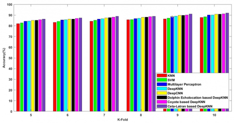
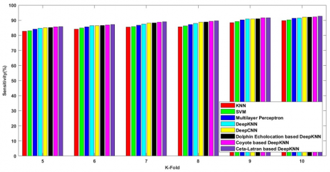
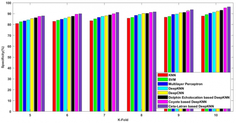
Figure 6 shows the comparative analysis on the k-fold values and the metrics are measured and enumerated. The observation shows that the cetalatran optimization attains higher values compared with the previously existing methods.
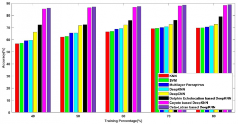
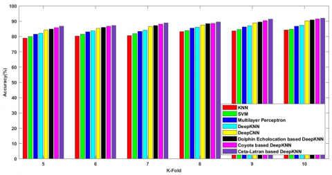
Figure 6a) shows the accuracy attained by the cetalatran optimization-deep CNN and the previous methods. Initially, the accuracy rate of the methods KNN, SVM, Multilayer Perceptron, Deep KNN, Deep CNN, Dolphin echolocation -deep KNN, Coyote-deep KNN and the cetalatran-optimization are measured and the obtained values are 87.733%, 88.459%, 90.080%, 90.145%, 90.866%, 90.883%, 91.232%, 91.879% respectively for the k-fold 10.
Figure 6b) explicit the sensitivity attained by the cetalatran-deep CNN with the k-fold 10 and the values for the methods KNN, SVM, Multilayer Perceptron, Deep KNN, Deep CNN, Dolphin echolocation-deep KNN, Coyote-deep KNN and the cetalatran-optimization are given by 89.871%, 90.309%, 91.335%, 91.650%, 92.105%, 92.166%, 92.269%, 92.736% respectively.
Figure 6c) denotes the specificity rate of the methods with k-fold value 10 and the values attained by the following methods are 87.809%, 89.198%, 90.434%, 91.328%, 92.316%, 92.995%, 95.290%, 95.951% respectively.
Comparative analysis on TP
The relation between the data and the attributes is given by the Training Percentage (TP) and is measured for the various methods described in detail in the below section.
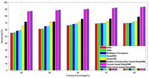
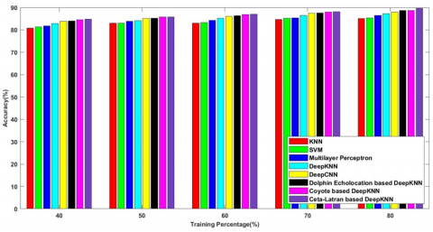
Figure 7a) shows the accuracy rate while measuring the values using the TP 80 and the values for the methods KNN, SVM, Multilayer Perceptron, Deep KNN, Deep CNN, Dolphin echolocation-deep KNN, Coyote-deep KNN and the cetalatran-optimization are measured and depicted as 85.117%, 85.419%, 86.505%, 87.365%, 87.987%, 88.670%, 88.700%, 89.126% respectively.
Figure 7b) denotes the sensitivity rate of the methods KNN, SVM, Multilayer Perceptron, Deep KNN, Deep CNN, Dolphin echolocation-deep KNN, Coyote-deep KNN, and the cetalatran-optimization for the TP 80 and are given by 87.392%, 88.107%, 88.488%, 88.720%, 89.915%, 90.205%, 92.705%, 93.392% respectively.
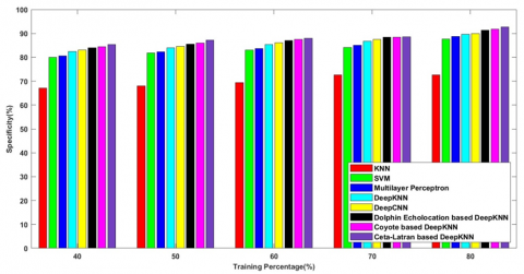
Figure 7c) enumerates the specificity rate of the methods KNN, SVM, Multilayer Perceptron, Deep KNN, Deep CNN, Dolphin echolocation-deep KNN, Coyote-deep KNN and the cetalatran-optimization and the values are listed as 72.773%, 87.584%, 88.738%, 89.665%, 90.008%, 90.811%, 91.850%, 92.772% respectively.
a)
b)
c)
Figure 6. Comparative analysis of band 8 multispectral image on k-fold a) accuracy b) sensitivity c) specificity
a)
b)
c)
Figure 7. Comparative analysis of band 8 multispectral image on TP a) accuracy b) sensitivity c) specificity
a)
b)
c)
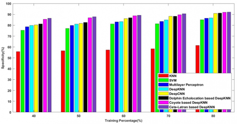
Figure 8. Comparative analysis of band 32 multispectral image on k-fold a) accuracy b) sensitivity c) specificity
a)
b)
c)
Figure 9. Comparative analysis of band 32 multispectral image on TP a) accuracy b) sensitivity c) specificity
5.4.4 Comparative analysis on band 32
The comparative analysis on band 32 with respect to the k-fold and the TP values are measured for proving the significance of the model.
Comparative analysis on k-fold
Figure 8 shows the comparative analysis on the k-fold values and the metrics of accuracy, sensitivity, and specificity are measured and enumerated. The observation shows that the cetalatran optimization attains higher values compared with the previously existing methods in terms of k-fold values.
Figure 8a) shows the accuracy attained by the cetalatran optimization-deep CNN and the previous methods. Initially the accuracy rate of the methods KNN, SVM, Multilayer Perceptron, Deep KNN, Deep CNN, Dolphin echolocation-deep KNN, Coyote-deep KNN, and the cetalatran-optimization are measured and the obtained values are 84.208%,84.767%, 86.713%, 87.407%, 90.218%, 90.883%, 91.517%, 92.023% respectively for the k-fold 10.
Figure 8b) explicit the sensitivity attained by the cetalatran-deep CNN with the k-fold 10 and the values for the methods KNN, SVM, Multilayer Perceptron, Deep KNN, Deep CNN, Dolphin echolocation-deep KNN, Coyote-deep KNN and the cetalatran-optimization are given by 88.264%, 88.962%, 90.191%, 90.739%, 91.728%, 92.290%, 93.122%, 93.829% respectively.
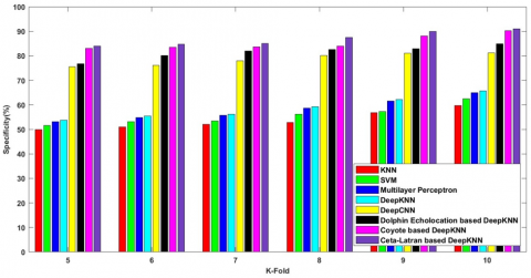
Figure 8c) denotes the specificity rate of the methods with k-fold value 10 and the values attained by the following methods are 59.735%, 62.435%, 65.006%, 65.648%, 81.141%, 84.967%, 90.218%, 91.050% respectively.
Comparative analysis on TP
The relation between the data and the attributes is given by the TP and is measured for the various methods described in detail in the below section.
Figure 9a) shows the accuracy rate while measuring the values using the TP 80 and the values for the methods KNN, SVM, Multilayer Perceptron, Deep KNN, Deep CNN, Dolphin echolocation-deep KNN, Coyote-deep KNN, and the cetalatran-optimization are measured and depicted as 69.612%, 69.770%, 70.496%, 71.457%, 72.648%, 78.983%, 88.255%, 88.818% respectively.
Figure 9b) denotes the sensitivity rate of the methods KNN, SVM, Multilayer Perceptron, Deep KNN, Deep CNN, Dolphin echolocation-deep KNN, Coyote-deep KNN, and the cetalatran-optimization for the TP 80 and are given by 69.140%, 69.337%, 69.409%, 70.859%, 72.091%, 78.781%, 92.806%, 93.443% respectively.
Figure 9c) enumerates the specificity rate of the methods KNN, SVM, Multilayer Perceptron, Deep KNN, Deep CNN, Dolphin echolocation-deep KNN, Coyote-deep KNN and the cetalatran-optimization and the values are listed as 61.356%, 84.984%, 86.415%, 86.779%, 90.944%, 91.139%, 91.875%, 92.053% respectively.
5.5 Comparative discussion
The comparative discussion is used to interpret the improvement rate attained by the Ceta latran-deep KNN over the previous existing state of art methods such as KNN, SVM, Multilayer Perceptron, Deep KNN, Deep CNN, Dolphin echolocation-deep KNN, Coyote-deep KNN shown in Table 2.
The attained rate shows that the cetalatran optimization-deep CNN method attains a higher improvement rate and for the simplified view the improvement rate attained with respect to the exiting coyote optimization-deep KNN is evaluated and the values are listed as follows: In the Band-8 with respect to the k-fold values, the improvement of 0.7043% in accuracy, 0.5034% in sensitivity, and 0.6896% in sensitivity is obtained. Similarly with respect to the TP improvement of 0.4776% in accuracy, 0.7356 in sensitivity, and 0.9932% in specificity is obtained. In the same way, the improvement rate of Band-32 is measured and the improvement rate of 0.5496% in accuracy, 0.7530% in sensitivity, and 0.9141% in specificity is obtained with respect to the K-fold and 0.6333% in accuracy, 0.6817 in specificity and 0.1935% in specificity with respect to the TP is obtained. The observations show that the cetalatran-deep KNN works more efficiently in all aspects of metrics values, which is more efficient.
Table 2. Comparative discussion of the cetalatran optimization-deep CNN
|
BAND-8 |
|||||||
|
Methods/Metrics |
K-fold |
TP |
|||||
|
Accuracy |
Sensitivity |
Specificity |
Accuracy |
Sensitivity |
Specificity |
||
|
KNN |
87.733 |
89.871 |
87.809 |
85.117 |
87.392 |
72.773 |
|
|
SVM |
88.459 |
90.309 |
89.198 |
85.419 |
88.107 |
87.584 |
|
|
Multilayer perceptron |
90.080 |
91.335 |
90.434 |
86.505 |
88.488 |
88.738 |
|
|
Deep KNN |
90.145 |
91.650 |
91.328 |
87.365 |
88.720 |
89.665 |
|
|
Deep CNN |
90.866 |
92.105 |
92.316 |
87.987 |
89.915 |
90.008 |
|
|
Dolphin echolocation - deep KNN |
90.883 |
92.166 |
92.995 |
88.670 |
90.205 |
90.811 |
|
|
Coyote - deep KNN |
91.232 |
92.269 |
95.290 |
88.700 |
92.705 |
91.850 |
|
|
Proposed |
91.879 |
92.736 |
95.951 |
89.126 |
93.392 |
92.772 |
|
|
BAND-32 |
|||||||
|
Methods/Metrics |
K-fold |
TP |
|||||
|
Accuracy |
Sensitivity |
Specificity |
Accuracy |
Sensitivity |
Specificity |
||
|
KNN [29] |
84.208 |
88.264 |
59.735 |
69.612 |
69.140 |
61.356 |
|
|
SVM [29] |
84.767 |
88.962 |
62.435 |
69.770 |
69.337 |
84.984 |
|
|
Multilayer perceptron [30] |
86.713 |
90.191 |
65.006 |
70.496 |
69.409 |
86.415 |
|
|
Deep KNN [31] |
87.407 |
90.739 |
65.648 |
71.457 |
70.859 |
86.779 |
|
|
Deep CNN [29] |
90.218 |
91.728 |
81.141 |
72.648 |
72.091 |
90.944 |
|
|
Dolphin echolocation - deep KNN [32] |
90.883 |
92.290 |
84.967 |
78.983 |
78.781 |
91.139 |
|
|
Coyote - deep KNN [33] |
91.517 |
93.122 |
90.218 |
88.255 |
92.806 |
91.875 |
|
|
Proposed |
92.023 |
93.829 |
91.050 |
88.818 |
93.443 |
92.053 |
|
The agricultural contribution plays an important role in the Indian economy and the occurrence of diseases in the leaves of the plants affects crop yields. Therefore, the improvement of various disease detecting technology is essential to attain a high yield. In this research, the plant leaf diseases are identified using the multispectral images through the utilization of the information collected from the vegetation indices NDVI, SAVI, OSAVI, NRI, GNDVI, SIPI, PSRI, EVI, DVI, RVI, LLSI. The multi-spectral image database has multiple layers of images that are separated on vegetation indices that resolve the time complexity. The conventional optimizers that were present assign the same weight whereas the cetalatran optimization effectively adjusts the weights the provides the optimal solution hence the time complexity is reduced and the convergence rate is improved. The preprocessing is performed to remove the noise caused due to the shadow of the images and the features are selected using a relief algorithm that is noise tolerant and that assigns to weight to every feature in the dataset. The cetalatran optimization-deep KNN utilizes this information and identifies the disease with higher efficiency through the optimization implemented in the classifier. The cetalatran-optimization effectively tuned the weight and bias of the parameter and provided an efficient output with 91.879% accuracy, 92.736% sensitivity, and 95.951% specificity. The detection of plant disease can be implemented in field management and crop health management.
[1] Akintayo, A., Tylka, G.L., Singh, A.K., Ganapathysubramanian, B., Singh, A., Sarkar, S. (2018). A deep learning framework to discern and count microscopic nematode eggs. Scientific Reports, 8(1): 1-11. https://doi.org/10.1038/s41598-018-27272-w
[2] Kaviyaraj, R., Uma, M. (2021). A survey on future of augmented reality with AI in education. In 2021 International Conference on Artificial Intelligence and Smart Systems (ICAIS), IEEE, pp. 47-52. https://doi.org/10.1109/ICAIS50930.2021.9395838
[3] Bock, C.H., Poole, G.H., Parker, P.E., Gottwald, T.R. (2010). Plant disease severity estimated visually, by digital photography and image analysis, and by hyperspectral imaging. Critical Reviews in Plant Sciences, 29(2): 59-107. https://doi.org/10.1080/07352681003617285
[4] Naik, H.S., Zhang, J., Lofquist, A., et al. (2017). A realtime phenotyping framework using machine learning for plant stress severity rating in soybean. Plant Methods, 13(1): 1-12. https://doi.org/10.1186/s13007-017-0173-7
[5] Zhang, J.P., Naik, H.S., Assefa, T., Sarkar, S., Reddy, R.V.C., Singh, A., Ganapathysubramanian, B., Singh, A.K. (2017). Computer vision and machine learning for robust phenotyping in genome-wide studies. Scientific Reports, 7(1): 44048. https://doi.org/10.1038/srep44048
[6] Gupta, G.K., Sharma, S.K., Ramteke, R. (2012). Biology, epidemiology and management of the pathogenic fungus macrophomina phaseolina (Tassi) Goid with special reference to charcoal rot of soybean (Glycine max (L.) Merrill). Journal of Phytopathology, 160(4): 167-180. https://doi.org/10.1111/j.1439-0434.2012.01884.x
[7] Nagasubramanian, K., Jones, S., Singh, A.K., Sarkar, S., Singh, A., Ganapathysubramanian, B. (2019). Plant disease identification using explainable 3D deep learning on hyperspectral images. Plant Methods, 15: 1-10. https://doi.org/10.1186/s13007-019-0479-8
[8] Pawlowski, M.L., Hill, C.B., Hartman, G.L. (2015). Resistance to charcoal rot identified in ancestral soybean germplasm. Crop Science, 55(3): 1230-1235. https://doi.org/10.2135/cropsci2014.10.0687
[9] Mengistu, A., Ray, J.D., Smith, J.R., Paris, R.L. (2007). Charcoal rot disease assessment of soybean genotypes using a colony-forming unit index. Crop Science, 47(6): 2453-2461. https://doi.org/10.2135/cropsci2007.04.0186
[10] Ampatzidis, Y., De Bellis, L., Luvisi, A. (2017). iPathology: Robotic applications and management of plants and plant diseases. Sustainability, 9(6): 1010. https://doi.org/10.3390/su9061010
[11] Tetila, E.C., Machado, B.B., Menezes, G.K., Oliveira, A.D.S., Alvarez, M., Amorim, W.P., Belete, N.A.D.S., Da Silva, G.G., Pistori, H. (2019). Automatic recognition of soybean leaf diseases using UAV images and deep convolutional neural networks. IEEE Geoscience and Remote Sensing Letters, 17(5): 903-907. https://doi.org/10.1109/LGRS.2019.2932385
[12] Cruz, A.C., Luvisi, A., De Bellis, L., Ampatzidis, Y. (2017). X-FIDO: An effective application for detecting olive quick decline syndrome with deep learning and data fusion. Frontiers in Plant Science, 8: 1741. https://doi.org/10.3389/fpls.2017.01741
[13] Cruz, A., Ampatzidis, Y., Pierro, R., Materazzi, A., Panattoni, A., De Bellis, L., Luvisi, A. (2019). Detection of grapevine yellows symptoms in Vitis vinifera L. with artificial intelligence. Computers and Electronics in Agriculture, 157: 63-76. https://doi.org/10.1016/j.compag.2018.12.028
[14] Pawlowski, M.L., Hill, C.B., Hartman, G.L. (2015). Resistance to charcoal rot identified in ancestral soybean germplasm. Crop Science, 55(3): 1230-1235. https://doi.org/10.2135/cropsci2014.10.0687
[15] Mengistu, A., Ray, J.D., Smith, J.R., Paris, R.L. (2007). Charcoal rot disease assessment of soybean genotypes using a colony-forming unit index. Crop Science, 47(6): 2453-2461. https://doi.org/10.2135/cropsci2007.04.0186
[16] Ampatzidis, Y., De Bellis, L., Luvisi, A. (2017). iPathology: Robotic applications and management of plants and plant diseases. Sustainability, 9(6): 1010. https://doi.org/10.3390/su9061010
[17] Cruz, A.C., Luvisi, A., De Bellis, L., Ampatzidis, Y. (2017). X-FIDO: An effective application for detecting olive quick decline syndrome with deep learning and data fusion. Frontiers in Plant Science, 8: 1741. https://doi.org/10.3389/fpls.2017.01741
[18] Cruz, A., Ampatzidis, Y., Pierro, R., Materazzi, A., Panattoni, A., De Bellis, L., Luvisi, A. (2019). Detection of grapevine yellows symptoms in Vitis vinifera L. with artifcial intelligence. Computers and Electronics in Agriculture, 157: 63-76. https://doi.org/10.1016/j.compag.2018.12.028
[19] Ampatzidis, Y., Partel, V. (2019). UAV-based high throughput phenotyping in citrus utilizing multispectral imaging and artificial intelligence. Remote Sensing, 11(4): 410. https://doi.org/10.3390/rs11040410
[20] Sladojevic, S., Arsenovic, M., Anderla, A., Culibrk, D., Stefanovic, D. (2016). Deep neural networks based recognition of plant diseases by leaf image classification. Computational Intelligence and Neuroscience, 2016. https://doi.org/10.1155/2016/3289801
[21] Fuentes, A., Yoon, S., Kim, S.C., Park, D.S. (2017). A robust deep-learning-based detector for real-time tomato plant diseases and pests recognition. Sensors, 17(9): 2022. https://doi.org/10.3390/s17092022
[22] Ferentinos, K.P. (2018). Deep learning models for plant disease detection and diagnosis. Computers and Electronics in Agriculture, 145: 311-318. https://doi.org/10.1016/j.compag.2018.01.009
[23] Multispectral Image Database. http://www2.cmp.uea.ac.uk/Research/compvis/MultiSpectralDB.htm.
[24] Kaveh, A., Farhoudi, N. (2013). A new optimization method: Dolphin echolocation. Advances in Engineering Software, 59: 53-70. https://doi.org/10.1016/j.advengsoft.2013.03.004
[25] Pierezan, J., Coelho, L.D.S. (2018). Coyote optimization algorithm: a new metaheuristic for global optimization problems. In 2018 IEEE congress on evolutionary computation (CEC), IEEE, pp. 1-8. https://doi.org/10.1109/CEC.2018.8477769
[26] Kaveh, A., Farhoudi, N. (2011). A unified approach to parameter selection in meta-heuristic algorithms for layout optimization. Journal of Constructional Steel Research, 67(10): 1453-1462. https://doi.org/10.1016/j.jcsr.2011.03.019
[27] Multispectral images of light leaf spot in oilseed rape. Mendeley Data. https://data.mendeley.com/datasets/ydmtggnzbw/1.
[28] Hatuwal, B.K., Shakya, A., Joshi, B. (2020). Plant leaf disease recognition using random forest, KNN, SVM and CNN. Polibits, 62: 13-19. https://doi.org/10.17562/PB-62-2
[29] Kumar, P.L., Goud, K.V.K., Kumar, G.V., Kumar, P.S. (2020). Enhanced weighted sum back propagation neural network for leaf disease classification. Materials Today: Proceedings. https://doi.org/10.1016/j.matpr.2020.09.514
[30] Abdulridha, J., Ampatzidis, Y., Kakarla, S.C., Roberts, P. (2020). Detection of target spot and bacterial spot diseases in tomato using UAV-based and benchtop-based hyperspectral imaging techniques. Precision Agriculture, 21: 955-978. https://doi.org/10.1007/s11119-019-09703-4
[31] Chen, T.T., Yang, W.G., Zhang, H.J., Zhu, B.Y., Zeng, R., Wang, X.Y., Wang, S.B., Wang, L.D, Qi, H.X., Lan, Y.B., Zhang, L. (2020). Early detection of bacterial wilt in peanut plants through leaf-level hyperspectral and unmanned aerial vehicle data. Computers and Electronics in Agriculture, 177: 105708. https://doi.org/10.1016/j.compag.2020.105708
[32] Abdulridha, J., Ampatzidis, Y., Roberts, P., Kakarla, S.C. (2020). Detecting powdery mildew disease in squash at different stages using UAV-based hyperspectral imaging and artificial intelligence. Biosystems Engineering, 197: 135-148. https://doi.org/10.1016/j.biosystemseng.2020.07.001
[33] Hu, G., Yin, C., Wan, M., Zhang, Y., Fang, Y. (2020). Recognition of diseased Pinus trees in UAV images using deep learning and AdaBoost classifier. Biosystems Engineering, 194: 138-151. https://doi.org/10.1016/j.biosystemseng.2020.03.021
[34] Yu, R., Luo, Y.Q., Zhou, Q., Zhang, X.D., Wu, D.W., Ren, L.L. (2021). A machine learning algorithm to detect pine wilt disease using UAV-based hyperspectral imagery and LiDAR data at the tree level. International Journal of Applied Earth Observation and Geoinformation, 101: 102363. https://doi.org/10.1016/j.jag.2021.102363
[35] Bhandari, M., Ibrahim, A.M.H., Xue, Q.W., Jung, J., Chang, A., Rudd, J.C., Maeda, M., Rajan, N., Neely, H., Landivar, J. (2020). Assessing winter wheat foliage disease severity using aerial imagery acquired from small unmanned aerial vehicle (UAV). Computers and Electronics in Agriculture, 176: 105665. https://doi.org/10.1016/j.compag.2020.105665