Ahmet Çelik*![]() | Semih Demirel
| Semih Demirel![]()
© 2023 IIETA. This article is published by IIETA and is licensed under the CC BY 4.0 license (http://creativecommons.org/licenses/by/4.0/).
OPEN ACCESS
Pneumonia poses a significant risk of mortality, particularly in individuals with compromised immune systems, necessitating early diagnosis and treatment to combat the disease effectively. In this study, we employed Multilayer Perceptron (MLP) and k-Nearest Neighbors (k-NN) machine learning (ML) algorithms to facilitate pneumonia diagnosis using preprocessed Chest X-ray images. Preprocessing steps, including Histogram Equalization, Mask R-CNN (Mask Region-Based Convolutional Neural Network), and Otsu thresholding, were successively performed on the images. Textural features were subsequently extracted from the Chest X-ray images and utilized as inputs for the classification algorithms. To address the imbalanced class problem in the training data, the Synthetic Minority Over-sampling Technique (SMOTE) was implemented. Classification evaluation metrics included accuracy, precision, recall, F1-Score, and AUC Score (Area Under Curve Score). The results revealed that the MLP algorithm outperformed the k-NN algorithm across all metrics. Furthermore, a comparison of the MLP and k-NN algorithms with previous studies in the literature demonstrated the superiority of the MLP algorithm, achieving an accuracy of 95.673%, F1-Score of 95.706%, and AUC Score of 99.006%. This study highlights the potential of employing the MLP algorithm for highly accurate pneumonia diagnosis using Chest X-ray images.
medical decision, X-ray image processing, histogram equalization, Otsu thresholding, machine learning, mask R-CNN, SMOTE technique
Pneumonia, a significant infectious disease affecting the lungs, can be caused by viruses or bacteria and may result in death if left untreated. This disease particularly impacts patients with weakened immune systems, rendering it especially lethal for children up to 5 years old and the elderly [1]. Consequently, early diagnosis is crucial to preventing mortality from pneumonia.
Chest X-ray images are routinely employed to diagnose pneumonia [2]. In clinical settings, radiologists examine these images in detail to determine the presence of pneumonia [3]. However, this diagnostic approach can be challenging when a radiologist is inexperienced or when faced with high patient density, resulting in increased workload, delayed diagnosis, and a higher error rate [4] (New Reference). The use of machine learning methods, a sub-branch of artificial intelligence, for X-ray image analysis and disease diagnosis may alleviate the workload of radiologists [3]. As a result, the accuracy and speed of pneumonia diagnosis could be enhanced by employing intelligent systems, thereby supporting the battle against pneumonia. Recent years have witnessed growing interest in machine learning systems for pneumonia diagnosis [5] (New Reference), although further research is required to verify their effectiveness and reliability [3].
In this study, binary classification of Chest X-ray images as normal and pneumonia-affected was conducted using two machine learning algorithms. First-order and second-order textural features were extracted from the images for use in the classification algorithms. To enhance classification performance, the rib cage was detected, and a segmentation mask was generated using Mask R-CNN [6]. Histogram Equalization was applied to improve image quality, and Otsu thresholding was utilized to facilitate feature extraction. Multilayer Perceptron and k-Nearest Neighbors algorithms were employed for classification. The Synthetic Minority Over-sampling Technique (SMOTE) was used to generate synthetic samples for the minority class, addressing the imbalanced class problem in the training data. Classification algorithms were compared using accuracy, precision, recall, and F1-Score metrics, additionally, the AUC Score was calculated by plotting the ROC Curve (Receiver Operating Characteristic Curve).
Especially in the last few years, the realization of automated medical image analysis using machine learning algorithms has become one of the most popular and accurate methods. To increase the accuracy of these methods and to improve them further, scientists have carried out many studies [7] (New Reference).
Chandra and Verma [8] presented a method based on feature extraction to detect pneumonia. Segmented lungs were used for feature extraction. Five different machine learning algorithms were used for classification. Logistic Regression achieved the highest accuracy with 95.63%. Subsequently, the multilayer perceptron also achieved good result with an accuracy of 95.39%.
Ayan and Ünver [9] trained the Xception [10] and VGG16 [11] model for pneumonia classification. They used transfer learning, fine-tuning and data augmentation methods in their study. According to the results, VGG16 and Xception achieved an accuracy of 87% and 82%, respectively.
Erdem and Aydin [12] used deep learning to detect pneumonia. Therefore, they proposed a new CNN model. They compared the proposed model with pre-trained models VGG16 and VGG19. Their proposed model achieved an accuracy of 88.62% and their proposed model outperformed VGG19 but underperformed VGG16.
Parveen and Khan [13] extracted features using the Histogram of Oriented Gradient (HOG) to classify pneumonia. They used Support Vector Machine (SVM), Decision Tree and Random Forest algorithms for classification. According to the results, the HOG+SVM model achieved the best performance with an accuracy of 95.3576%.
Manickam et al. [14] aimed at detecting pneumonia using deep learning models. They used the ResNet50 [15] InceptionV3 and InceptionResNetV2 models and preprocessing steps were performed to improve performance. The best results were obtained using the ResNet50 model with 93.06% accuracy.
Beena Ullala Mata et al. [16] used Otsu thresholding, K-means clustering, and spherical thresholding algorithms to segment X-ray images. Then the contour detection algorithm was applied, which helps to detect the lung border. The detected area was used to classify normal lung from pneumonia affected lung.
Haralick et al. [17] developed a method called Gray Level Co-Occurrence Matrix (GLCM). In the study, 14 different second-order texture features used for texture classification.
Ramola et al. [18] has written a comprehensive report on GLCM's tissue classification technique and the evolution of deep perception models.
Smart pneumonia detection methods are applied on Chest X-ray image datasets from both public and private sources [19]. The dataset publicly available on Kaggle was used in the study [20]. The dataset contains 3 folders: train, test, validation. Each folder is divided into 2 subfolders for normal and pneumonia. The pneumonia folder contains Chest X-ray images of Bacterial Pneumonia caused by bacteria and Viral Pneumonia caused by viruses. It is worth considering that the use of two different types of pneumonia data could potentially affect the study's findings. Any known or potential differences between these subtypes should be accounted for in the analysis. However, the study's main focus was on developing a deep learning model to classify normal and pneumonia chest X-ray images, and the use of both bacterial and viral pneumonia images was still relevant for achieving this goal.
Table 1 gives the class and number details of the dataset. In this study, we used only train and test folders. There is an imbalanced class problem in the training data between normal and pneumonia classes. Despite the class imbalance issue and use of only two data subsets, the study's results can still provide valuable insights for the diagnosis and treatment of pneumonia.
SMOTE method used to address the imbalanced class problem. In this study, SMOTE was used to address this problem and 2534 synthetic samples were generated with SMOTE using normal images in the train folder. Specifically, the SMOTE [21] algorithm was used with default settings to oversample the normal class and increase its sample size from 1341 to 3875. This resulted in a balanced training set, which contained equal numbers of normal and pneumonia samples. The use of SMOTE was effective in addressing the class imbalance issue between the normal and pneumonia classes. In this way, the imbalanced class problem between normal and pneumonia classes in the training data was addressed. Details of the number of samples after SMOTE are given in Table 2.
Table 1. The class and number details of the dataset
|
Dataset |
Normal |
Pneumonia |
Total |
|
Train |
1341 |
3875 |
5216 |
|
Test |
234 |
390 |
624 |
|
Validation |
8 |
8 |
16 |
|
Total |
1583 |
4273 |
5856 |
Table 2. Details of the number of samples after SMOTE
|
Dataset |
Normal |
Pneumonia |
Total |
|
Train |
3875 |
3875 |
7750 |
|
Test |
234 |
390 |
624 |
|
Validation |
8 |
8 |
16 |
|
Total |
4117 |
4273 |
8390 |
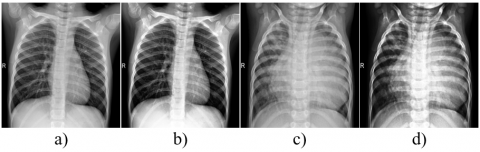
Figure 1 shows examples of images. Images belong to children aged 1-5 and were obtained from Guangzhou Women’s and Children’s Medical Center.
|
a) |
b) |
c) |
Figure 1. Examples of images from the dataset (a)Normal Chest X-ray, (b) Bakterial Pneumonia, (c)Viral Pneumonia
In this study, Histogram Equalization, Mask R-CNN and Otsu thresholding preprocessing steps were performed on each of the train and test Chest X-ray images, respectively.
4.1 Histogram equalization
The distribution of pixel intensities of an image is shown in histogram graph [22]. Information about the contrast of an image can be obtained using the histogram. The pixel intensities of a low-contrast image are distributed over a short range in the histogram graph. Histogram Equalization is an image processing technique that can enhance the contrast of an image by redistributing its pixel intensities [23] (New Reference). The algorithm involves calculating the cumulative distribution function (CDF) of the image, then mapping each pixel value to a new value using a transfer function based on the CDF [24] (New Reference). This results in a more evenly distributed histogram, and an image with improved contrast. If Histogram Equalization is performed on an image, the pixel intensities of the image are distributed over a broader range in the histogram graph [25]. In this way, the quality of the image is improved by enhancing the contrast using Histogram Equalization.
In this study, Histogram Equalization was performed for each of the original images in order to improve the quality of the image. Figure 2 shows images after Histogram Equalization.
Figure 2. Histogram equalization on chest X-ray images. (a) Original normal chest X-ray, normal chest X-ray after histogram equalization, (c) Original pneumonia chest X-ray, (d) Pneumonia chest X-ray after histogram equalization
In Figure 2, the original image appears dull and lacks contrast. However, after applying Histogram Equalization, the image is brighter, and the details of the lung structures are more prominent.
4.2 Mask R-CNN
Mask R-CNN can achieve great success for object recognition and segmentation mask generation. Mask R-CNN needs to perform two stages for this great success. In the first stage, bounding box proposals, which are expected to contain an object, are generated on the feature maps obtained by using the backbone network in the input image. In the RoI (Region of Interest) Align layer, the value of the pixel points is calculated by performing bilinear interpolation on the feature map to get the precise location of RoIs. In the second stage, the generation of the segmentation mask, the classification of the objects, and the generation of the bounding box are performed in parallel [26].
4.2.1 Image annotation and labeling
In this study, a segmentation mask was generated for the rib cage using Mask R-CNN. To train the Mask R-CNN, 1000 (500 normal, 500 pneumonia) and 400 (200 normal, 200 pneumonia) contrast enhanced Chest X-ray images were used for training and validation, respectively. The Mask R-CNN model is trained to detect the rib cage. Therefore, Chest X-ray images were annotated using the VGG Image Annotator (VIA) to determine the boundaries of the ribcage. In each Chest X-ray image, the boundaries of the rib cage were drawn manually using the Polygon Shape tool and labeled as “rib cage”.
4.2.2 Training details of mask R-CNN
In this study, Mask R-CNN model developed by Matterport, Inc. was used. The default hyper parameters of the model were adapted to our study. In this study, transfer learning was applied by using pre-trained weights on the MSCOCO (Microsoft Common Objects in Context) dataset [27]. ResNet101-FPN (ResNet101-Feature Pyramid Network) was used as a backbone network. In the training of the model, the loss value converged in the 30th epoch. Therefore, the model was trained for 30 Epochs. Each epoch consists of 100 steps. The Mask R-CNN model was trained using the GPU (Graphics Processing Unit) on Google Collaborator.
4.2.3 Loss function
In this study, loss functions calculate the loss value taking into account the true value and the predicted value. The training of the model works better by minimizing the loss value [28]. In Mask R-CNN, the total loss value consists of five losses. These are obtained at the output of the RPN (Region Proposal Network) stage which obtained at the output of Mask R-CNN.
The loss function of the RPN stage is given in Eq. (1).
$\begin{gathered}L\left(L_{c l s}, L_{r e g}\right)=\frac{1}{N_{c l s}} \sum L_{c l s}\left(y_i, p_i\right)+ \lambda \frac{1}{N_{r e g}} \sum L_{r e g}\left(t_i, t_i^{\prime}\right)\end{gathered}$ (1)
Lcls and Lreg represent the classification loss and regression loss, respectively. Ncls ve Nreg represent the number of anchors that are classified and regressed, respectively. Lcls is given in Eq. (2).
$L_{c l s}\left(y_i, p_i\right)=\sum_i-\left[y_i \log \left(p_i\right)+\left(1-y_i\right) \log (1-p_i)\right]$ (2)
yi and pi are ground truth and predicted value, respectively. Lreg is given in Eq. (3).
$L_{r e g}\left(t_i, t_i^{\prime}\right)=\sum_{i \in\{x, y, w, h\}} \quad \operatorname{smooth}_{L 1}\left(t_i-t_i^{\prime}\right)$ (3)
$t_i t_i^{\prime}$ are ground truth and predicted bounding boxes, respectively. {x, y, w, h} are the coordinates of the bounding boxes.
In Figure 3, the training and validation loss values of the Mask R-CNN model are shown as the sum of 5 losses. The graph indicates a gradual decrease in loss values during the training process. The training and validation loss values at the completion of training are 0.1738 and 0.2010, respectively. Notably, after the 20th epoch, there is only a slight decrease in the loss values, suggesting that the model is converging. Therefore, we continued training the Mask R-CNN model for a total of 30 epochs. Upon reaching the 30th epoch, we observed that the loss values were quite small, indicating that the model was performing well. This convergence of the loss value at the 30th epoch suggests that the model has reached an optimal state, and further training may not lead to significant improvements in the performance. Convergence of the loss value occurs when the loss function stops decreasing significantly and reaches a stable value [29]. This means that the model has learned all it can from the training data and is no longer improving significantly. At this point, the model can be considered to have converged. When the loss value has converged, it means that the model has learned the best possible set of weights and biases that minimize the loss function. This is an indication that the model has learned to generalize well on the training data and is ready to be tested on new data.
In this study, a segmentation mask for the rib cage was generated using Mask R-CNN on contrast enhanced Chest X-ray images. Only one pixel value was assigned to the region except for the rib cage, which is the background. By means of Mask R-CNN, the effect of background organs on classification performance is minimized. Figure 4, shows examples of segmentation mask generated for the rib cage.
Figure 3. Training and validation loss graphs in 30 epoch
Figure 4. Mask R-CNN on a normal Chest X-ray image: (a) d Normal Chest X-ray, (b) A segmentation mask for the rib cage, (c) Result of the Mask R-CNN on a normal Chest X-ray image
4.3 Otsu thresholding
The OTSU algorithm is used to subdividing the original image into its foreground and its background image through the use of a threshold. Using the histogram of the image, an optimal threshold is derived between the classes. Optimum threshold value is greater than the portion gray value of image is called the background; otherwise, the portion is called the foreground. As result of the segmentation of gray image is separated the foreground and background [30]. In thresholding, a gray scale image is converted to black and white in a binary image.
In this study, Otsu thresholding was performed on each of the segmented Chest X- Ray image. In this way, healthy regions were segregated using Otsu thresholding. Figure 5 shows images after Otsu thresholding. After Otsu thresholding, black pixels represent the healthy region, white pixels represent the pneumonia-infected region or other organs and gray pixels represent the background. Otsu thresholding was used to facilitate feature extraction. However, it is important to note that Otsu thresholding is just one method among many available for threshold segmentation.
Figure 5. Otsu thresholding on Chest X-ray images (a) Before Otsu thresholding on Seg- mented Normal Chest X-ray, (b) After Otsu thresholding on Segmented Normal Chest X-ray, (c) Before Otsu thresholding on Segmented Pneumonia Chest X-ray, (d) After Otsu thresholding on Segmented Pneumonia Chest X-ray
In this study, textural features were extracted on each Chest X-ray image after preprocessing. In Machine Learning algorithms, imbalanced class problem in the training data affects classification performance. Therefore, the imbalanced class problem was addressed by generating new synthetic samples with SMOTE using the calculated textural features. In the last step, Chest X-ray images were classified using the textural features extracted for the classification algorithms. In this study, the flow chart of the proposed approach that performs binary classification as normal and pneumonia is shown in Figure 6.
Figure 6. Flow chart of proposed approach for pneumonia classification
5.1 Textural feature extraction
Shapes and patterns in an image are called textural features of the image. Distinctive textural measures are extracted by analyzing textural features. Calculated textural measures are used as features in machine learning classification algorithms to classify images. These textural measures are first-order textural measures, second-order textural measures and higher-order textural measures. The relationship between pixels in first-order texture measures is calculated using the original pixel intensities without considering the relationship between adjacent pixels. Second-order texture measures examine the relationship between two groups of pixels. Third and higher-order texture measures are theoretically possible, but are not used due to the difficulty in computation and interpretation [31]. Therefore, in this study, we used first order and second order textural measures. These measures were calculated on Chest X-ray images after Otsu thresholding. These calculated textural measures were used as features for classification algorithms.
5.1.1 First order textural measures
First-order textural measures are extracted using the original pixel values in an image. In the first-order textural measures, the relationship of pixels to each other is not taken into account [32].
In this study, three first-order textural measures were calculated. These textural measures are mean, variance, and the ratio of the number of white pixels to the number of black pixels. Mean and Variance were calculated using the entire Chest X-ray image and we used Scipy [33], which is a Python library, to calculate the mean and variance. Scipy is a library of algorithms that solve problems such as optimization, algebraic, differential and statistical. The mean is the sum of the gray pixel intensities of an image divided by the total number of pixels are calculated with the following Eq. (4). The variance indicates how the gray pixel intensities of an image spread around the mean is calculated with the following Eq. (5).
$\mu=\left(\frac{1}{M \times N}\right) \sum_{i=0}^{M-1} \sum_{j=0}^{N-1}P$ (4)
$\sigma^2=\left(\frac{1}{M \times N}\right) \sum_{i=0}^{M-1} \sum_{j=0}^{N-1} (P(i, j)-\mu)^2$ (5)
µ is the mean of the image. The pixel density of location (i, j) is P(i, j) and MxN is the resolution of the image. The Ratio of The Number of White Pixels to The Number of Black Pixels. In this study, the ratio of the number of white pixels to the number of black pixels on Chest X-ray images after Otsu thresholding was used as a feature for classification. This ratio is given in Eq. (6).
$b w_R=\frac{\text { wpixel }_c}{\text { Bpixel }_c}$ (6)
bwR, ratio of the white pixels count to the black pixels count, Wpixelc, white pixels count in lung area, Bpixelc, black pixels count in lung area.
5.1.2 Second order textural measures
In the second-order textural measure, the relation-ships of the pixels are analyzed [34].
In this study, we extracted 5 textural features: ASM, Correlation, Contrast, Homogeneity and Dissimilarity. These textural features were calculated using the entire Chest X-ray image and we used Scikit-Image [18], which is a Python library, to calculate the textural features. Scikit-Image is a library that provides algorithms for image processing and feature extraction.
ASM (Angular Second-Moment): A small number of gray levels in an image indicate uniformity between pixels. The greater the uniformity is higher the sum of the squares of the P(i, j) entries are calculated with the following Eq. (7).
$ASM=\sum_{i=0}^{M-1} \sum_{j=0}^{N-1} P(i, j)^2$ (7)
Correlation: Correlation indicates whether a pixel has a linear connection with another neighboring pixel is calculated with the following Eq. (8).
$correlation=\sum_{i=0}^{M-1} \sum_{j=0}^{N-1} P(i, j) \left[\frac{\left(i-\mu_i\right)\left(j-\mu_j\right)}{\sqrt{\sigma_i^2 \sigma_j^2}}\right]$ (8)
Contrast: Contrast is greater when there is more variation between one pixel and another in an image is calculated with the following Eq. (9).
$contrast=\sum_{i=0}^{M-1} \sum_{j=0}^{N-1} P(i, j) (i-j)^2$ (9)
Homogeneity: A lower variation between pixels is an indication of homogeneity and this ensures higher homogeneity is calculated with the following Eq. (10).
$homogeneity=\sum_{i=0}^{M-1} \sum_{j=0}^{N-1} \frac{P(i, j)}{1+(i-j)^2}$ (10)
Dissimilarity: Dissimilarity increases linearly rather than exponentially as variation between pixels increases are calculated with the following Eq. (11).
$dissimilarity=\sum_{i=0}^{M-1} \sum_{j=0}^{N-1} P(i, j) \vee i-j \vee$ (11)
In (11), P(i, j) denotes an entry at location (i, j) in a GLCM.M and N are the number of rows and columns of the GLCM, respectively.
5.2 Synthetic Minority Over-sampling Technique (SMOTE)
One of the problems affecting classification performance is imbalanced class. Classification performance is disadvantageous for the minority class in the imbalanced class problem [35]. One way to overcome this problem is oversampling. In the oversampling method, this problem is overcome by adding samples to the minority class. In SMOTE, which is an oversampling method, the needed samples are created by using the samples of the minority class with the help of the k-Nearest Neighbors algorithm [36].
In this study, the imbalanced-learn [37], which is a Python library, was used for SMOTE. Imbalanced-learn is a library that provides solutions to imbalanced class problems and contains algorithms such as SMOTE, ADASYN. For the K-Nearest Neighbors algorithm, k=25 was used. Grid-Search algorithm was used to determine the k value.
5.3 Classification
In this study, Multilayer Perceptron and K-Nearest Neighbors algorithms were used for classification.
5.3.1 Multilayer Perceptron (MLP)
MLP can overcome difficult classification problems thanks to its connections in its layers. Layers consist of a series of perceptron. Perceptron in the first layer receive feature values from the dataset. The perceptron in the hidden layers process the values from the previous layer with mathematical calculations. Each perceptron in the output layer generates an output. The number of perceptron in the layers vary according to the problem [38], Figure 7 shows a basic MLP.
Figure 7. Layers and perceptions of a basic MLP
In Figure 7, the number of perceptron in the layers is 2, 3 and 1, respectively. x1 and x2 represent the input values. The mathematical model of a perceptron is calculated with the following Eq. (12).
$y=f\left(\sum_{i=0}^{n-1} w_i x_i+b\right)$ (12)
n-1 is the number of inputs, wi is the weight of the i th connection, xi is the input value of the i th connection, b is the bias value, and f is the activation function and y is the output value of the perceptron. An output value is obtained at the end of the output layer of the MLP neural network. Using the obtained output and the target, the difference between each other is calculated. In order to minimize the difference, the weights and bias values are adjusted by using the Back propagation algorithm [39].
In this study, Scikit-Learn, which is a Python library [40], was used to create the MLP model. Scikit-Learn is a library of algorithms for Machine Learning. In addition to an input and an output layer, 3 hidden layers are used to create this model. The numbers of perceptron in the hidden layers are 8, 8 and 2, respectively. Since this study aimed at a binary classification, the sigmoid activation function was used as the activation and is calculated with the Eq. (13)
$f(x)=\frac{1}{1+e^{-x}}$ (13)
The Adam [41] optimization algorithm was used for the solver. 0.0001 was used for the Alpha which is the regularization hyper parameter. The Grid Search algorithm can find optimal values for hyper parameters. Stochastic Optimization [42] (New Reference) algorithms are widely used in machine learning and signal processing methods.
In this study, this algorithm was used for hyper parameters such as the number of hidden layers, the number of perceptron in each hidden layer, batch size, alpha, learning rate in it, and random state. Default values were used for other hyper parameters.
5.3.2 K-Nearest Neighbors(k-NN)
K-Nearest Neighbors classifies the samples by calculating the distance from each other in the feature space [43]. For a test sample, the closest training samples are found according to the k value. The class with the greater number of samples among the found training samples includes the test sample. There are different metrics for distance measurement. Euclidean, Manhattan and Minkowski, which are examples of these metrics, are given in Eqns. (14), (15) and (16).
$d(a, b)=\sqrt{\sum_{i=1}^n \left(x_i-y_i\right)^2}$ (14)
$d(a, b)=\sum_{i=1}^n \left|x_i-y_i\right|$ (15)
$d(a, b)=\left(\sum_{\mathrm{i}=1}^{\mathrm{n}}\left|\mathrm{x}_{\mathrm{i}}-\mathrm{y}_{\mathrm{i}}\right|^{\mathrm{p}}\right)^{\frac{1}{\mathrm{p}}}$ (16)
d is the distance, a is the test sample, b is the training sample, n is the number of features in the dataset, xi is the variable of the test sample, yi is the variable of the training sample, p is the power parameter for Minkowski.
In this study, Scikit-Learn were used for k-NN. Euclidean was used as the distance measurement metric. Selecting the optimal value of k improves the classification performance. Therefore, values between 1 and 31 were tested for k and the best classification performance was achieved with k=9. That’s why 9 was used for the n neighbors hyper parameter in the Scikit-Learn. Default values were used for other hyper parameters.
The aim of this study is to perform binary classification as normal and pneumonia. Multilayer Perceptron and K-Nearest Neighbors algorithms were trained for classification. The trained classification algorithms were tested on 624 Chest X-ray images.
Confusion matrices of classification algorithms are shown in Figure 8. In Figure 8, True negative values of MLP and k-NN are 225 and 223, true positive values are 368 and 341, false positive values are 9 and 11, false negative values are 22 and 49 respectively.
Figure 8. Confusion matrices
Figure 9 shows the ROC curves of MLP and k-NN. The yellow solid line and the blue solid line show the ROC Curve of the MLP and k-NN, respectively. A curve close to the dashed line is indicative of poor classification performance. The curve of k-NN is closer to the dashed line than the curve of MLP. Therefore, the AUC Score of MLP is higher than the AUC Score of k-NN and MLP outperformed k-NN.
Figure 9. The ROC curves of MLP and k-NN
In this study, precision, recall and F1 Score were calculated for both labels and the weighted average was calculated. Since the weighted average is calculated, accuracy and recall values are equal. A comparison of classification algorithms using performance evaluation metrics are given in Table 3.
Table 3. The test results of MLP and k-NN
|
|
Accuracy (%) |
Precision (%) |
Recall (%) |
F1-Score (%) |
AUC Score (%) |
|
Multilayer Perceptron |
95.6731 |
95.9625 |
95.6731 |
95.7061 |
99.0061 |
|
k-Nearest Neighbors |
91.0256 |
91.702 |
91.0256 |
91.1209 |
96.5702 |
Table 4. Comparison of MLP and k-NN with previous studies the literature
|
Paper |
Method |
Accuracy (%) |
Precision (%) |
Recall (%) |
F1-Score (%) |
AUC Score (%) |
|
Chandra and Verma[8] |
MLP |
95.388 |
97.462 |
93.204 |
95.285 |
95.4 |
|
Ayan and Ünver [9] |
VGG16 |
87 |
- |
82 |
- |
- |
|
Erdem and Aydın [12] |
CNN |
88.62 |
86.16 |
97.43 |
91.45 |
- |
|
Parveen and Khan [13] |
HOG+SVM |
95.357 |
95.026 |
94.507 |
94.76 |
- |
|
Manickam et al. [14] |
ResNet50 |
93.06 |
88.97 |
96.78 |
92.71 |
93.0 |
|
Proposed System |
MLP |
95.673 |
95.962 |
95.673 |
95.706 |
99.006 |
|
k-NN |
91.025 |
91.702 |
91.025 |
91.120 |
96.570 |
In the Table 3, the Multilayer Perceptron outperformed K-Nearest Neighbors in all metrics. The accuracy values of MLP and k-NN are 95.673% and 91.025%, respectively. This means that MLP predicted more samples correctly. The precision value of MLP is higher than the precision value of k-NN. Therefore, MLP is better at classifying correctly for normal labeled samples. Likewise, the recall value of MLP is higher than the recall value of k-NN. Therefore, MLP is better at classifying correctly for pneumonia labeled samples. Since the precision and recall values of MLP are higher than k-NN, the F1-Score of MLP is higher than k-NN. The F1-Score of MLP and k-NN are 95.706% and 91.120%, respectively. The maximum value of the AUC Score is 1. The AUC Score of MLP is 99.006%, which is very close to 1. In addition, the AUC Score of k-NN is 96.520%. Therefore, MLP outperformed k-NN for pneumonia classification. Previous studies classifying pneumonia in the literature and our models were compared in Table 4.
In the Table 4, the accuracy of the MLP model proposed by Chandra and Verma [8] is 95.388%. Our MLP model has a higher accuracy of 95.673%. Therefore, out MLP model correctly predicted more samples than other studies. The precision of the MLP model proposed by Chandra and Verma [8] is 97.462%, which is the best when compared to other studies. This means that Chandra and Verma [8] is the article that best classifies the samples with normal label. The recall of the CNN model proposed by Erdem and Aydın [12] is 97.43%, which is higher than other studies. This means that Erdem and Aydın [12] is the article that best classifies samples with pneumonia label. In Chandra and Verma [8], the recall value is less than the precision value, in Erdem and Aydın [12] recall value is greater than precision value. Therefore, the F1-Score values in Chandra and Verma [8] and Erdem and Aydın [12] are small values. However, the precision and recall values of our MLP model are balanced high. Therefore, the F1-Score of our MLP model is higher than the F1-Score of Chandra and Verma [8] and Erdem and Aydın [12]. The F1-Score and AUC Score of our MLP model are 95.706% and 99.006%, respectively, and these values are higher than other studies. A high AUC Score indicates good classification performance at different thresholds. Therefore, our MLP model is better than other studies. As a result, our MLP model outperformed other studies in AUC Score, accuracy and F1-Score.
The accuracy and recall of the VGG16 model proposed by Ayan and Ünver [9] are 82% and 87%, respectively. The accuracy of the HOG+SVM model proposed by Parveen, and Khan [13] is 95.359%. While this value is higher than the accuracy of our k-NN model, it is very close to the accuracy of our MLP model. The accuracy and recall of the ResNet50 model proposed by Manickam et al. [14] are 93.06% and 96.78%, respectively. In terms of recall, it is higher than the recall of our MLP and k-NN models, and very close to the recall of the CNN model proposed by Erdem and Aydın [12].
A limitation of this study is the imbalance between the normal and pneumonia subfolders in the train folder and the insufficient number of images for both subfolders. In this study, SMOTE was used to solve this problem. However, in the original dataset, if the images were evenly distributed in the train folder and there were more images, the classification performance could be improved and more reliable results could be obtained.
In this study, binary classification of Chest X-ray images was performed. In the study, preprocessing steps of Histogram Equalization, Mask R-CNN and Otsu thresholding were performed. First-order and second-order textural features extracted after preprocessing steps were used as features for classification algorithms. In addition, SMOTE was used to address the imbalanced class problem in the training data.
In this study, Multilayer Perceptron and K-Nearest Neighbors algorithms were used for classification and the performances of the algorithms were compared. As a result, Multilayer Perceptron is better than K-Nearest Neighbors algorithm in all metrics. In addition, the proposed MLP and k-NN models were compared with previous studies in the literature. The proposed MLP model achieved an accuracy of 95.673%, F1-Score of 95.706% and AUC Score of 99.006%. These results are the best when compared with previous studies.
In future studies, it is aimed to detect pneumonia due to COVID-19 by using other Machine Learning classification algorithms on Chest X-ray images. In addition, a study comparing machine learning algorithms and deep learning models for Chest X-ray classification is aimed in future studies. In addition, in clinical settings, it may be useful to conduct new studies on how radiologists perceive and interact with such intelligent diagnostic systems.
|
MLP |
Multilayer Perceptron |
|
SVM |
Support Vector Machine |
|
k-NN |
k-Nearest Neighbors |
|
ML |
Machine Learning |
|
Mask R-CNN |
Mask Region-Based Convolutional Neural Network |
|
SMOTE |
Synthetic Minority Over-sampling Technique |
|
AUC |
Area Under Curve |
|
HOG |
Histogram of Oriented Gradient |
|
DT |
Decision Tree |
|
ROC |
Receiver Operating Characteristic |
|
RoI |
Region of Interest |
|
MSCOCO |
Microsoft Common Objects in Context |
|
GPU |
Graphics Processing Unit |
|
FPN |
Feature Pyramid Network |
|
GLCM |
Mac Gray Level Co-Occurrence Matrix |
|
ASM |
Angular Second-Moment |
|
COVID-19 |
Coronavirus 2019 |
|
ML |
Machine Learning |
[1] Fernandes, V., Junior, G., Paiva, A., Silva, A., Gattass, M. (2021). Bayesian convolutional neural network estimation for pediatric pneumonia detection and diagnosis. Computer Methods and Programs in Biomedicine, 208(2): 106259. https://doi.org/10.1016/j.cmpb.2021.106259
[2] Yao, S., Chen, Y., Tian, X., Jian, X. (2021). Pneumonia detection using an improved algorithm based on faster R-CNN. Computational and Mathematical Methods in Medicine, 2021: 8854892. https://doi.org/10.1155/2021/8854892
[3] Tümen, V. (2022). SpiCoNET: A hybrid deep learning model to diagnose COVID-19 and pneumonia using chest X-ray images. Traitement du Signal, 39(4): 1169-1180. https://doi.org/10.18280/ts.390409
[4] Szepesi, P., Szilagyi, L. (2022). Detection of pneumonia using convolutional neural networks and deep learning. Biocybernetics and Biomedical Engineering, 42(3): 1012-1022. https://doi.org/10.1016/j.bbe.2022.08.001
[5] Wang, Y., Hargreaves, C.A. (2022). A review study of the deep learning techniques used for the classification of chest radiological images for COVID-19 diagnosis. International Journal of Information Management Data Insights, 2(2): 100100. https://doi.org/10.1016/j.jjimei.2022.100100
[6] Bi, X., Hu, J., Xiao, B., Li, W., Gao, X. (2023). IEMask R-CNN: Information-enhanced Mask R-CNN. In IEEE Transactions on Big Data, 9(2): 688-700. https://doi.org/10.1109/TBDATA.2022.3187413
[7] Ngong, I.C., Baykan, N.A. (2023). Different deep learning based classification models for COVID-19 CT-scans and lesion segmentation through the cGAN-UNet hybrid method. Traitement du Signal, 40(1): 1-20. https://doi.org/10.18280/ts.400101
[8] Chandra, T., Verma, K. (2020). Pneumonia detection on chest X-ray using machine learning paradigm. In: 2020 Proceedings of 3rd International Conference on Computer Vision and Image Processing (CVIP), pp. 21-33. https://doi.org/10.1007/978-981-32-9088-4_3
[9] Ayan, E., Ünver, H.M. (2019). Diagnosis of pneumonia from chest X-ray images using deep learning. In: 2019 Scientific Meeting on Electrical-Electronics Biomedical Engineering and Computer Science (EBBT), Istanbul, Turkey, pp. 1-5. https://doi.org/10.1109/EBBT.2019.8741582
[10] Chollet, F. (2017). Xception: deep learning with depthwise separable convolutions. In: 2017 IEEE Conference on Computer Vision and Pattern Recognition (CVPR), Honolulu, HI, USA, pp. 1800-1807. https://doi.org/10.1109/CVPR.2017.195
[11] Bozkurt, F. (2021). Derin öğrenme tekniklerini kullanarak akciğer X-ray görüntülerinden COVID-19 tespiti. Avrupa Bilim ve Teknoloji Dergisi, 24: 149-156. https://doi.org/10.31590/ejosat.898385
[12] Erdem, E., Aydın, T. (2021). Detection of pneumonia with a novel CNN-based approach. Sakarya University Journal of Computer and Information Sciences, 4(1): 26-34. https://doi.org/10.35377/saucis.04.01.787030
[13] Parveen, S., Khan, K. (2020). Detection and classification of pneumonia in chest X-ray images by supervised learning. In: 2020 IEEE 23rd International Multitopic Conference (INMIC), Bahawalpur, Pakistan, pp. 1-10. https://doi.org/10.1109/INMIC50486.2020.9318118
[14] Manickam, A., Jiang, J., Zhou, Y., Sagar, A., Soundrapandiyan, R., Samuel, D.J. (2021). Automated pneumonia detection on chest X-ray images: A deep learning approach with different optimizers and transfer learning architectures. Measurement, 184: 109953. https://doi.org/10.1016/j.measurement.2021.109953
[15] Cannata, S., Paviglianiti, A., Pasero, E., Cirrincione, G., Cirrincione, M. (2022). Deep learning algorithms for automatic COVID-19 detection on chest X-ray images. In IEEE Access, 10: 119905-11991. https://doi.org/10.1109/ACCESS.2022.3221531
[16] Beena Ullala Mata, B.N., Rishika, I.S., Nikita, J., Kaliprasad, C.S. (2021). Detection of pneumonia using chest X-ray images and image processing algorithms: A comparative study. Journal of Image Processing and Artificial Intelligence, 7: 31-40. https://doi.org/10.46610/JOIPAI.2021.v07i03.005
[17] Haralick, R., Shanmugam, K., Dinstein, I. (1973). Textural features for image classification. IEEE Transactions on Systems, Man, and Cybernetics, 3(6): 610-621. https://doi.org/10.1109/TSMC.1973.4309314
[18] Ramola, A., Shakya, A., Pham, D. (2020). Study of statistical methods for texture analysis and their modern evolutions. Engineering Reports, 2(4): e12149. https://doi.org/10.1002/eng2.12149
[19] Zhang, X., Han, L., Sobeih, T., Han, L., Dempsey, N., Lechareas, A.T., Chen, H., White, S., Zhang, D. (2023). CXR-Net: A multitask deep learning network for explainable and accurate diagnosis of COVID-19 pneumonia from Chest X-ray images. IEEE Journal of Biomedical and Health Informatics, 27(2): 980-991. https://doi.org/10.1109/JBHI.2022.3220813
[20] Çelik, A., Demirel, S. (2022). Otsu ve Ridler-Calvard Görüntü İşleme Yöntemlerinin Zatürre Tespitinde Kullanılması. Muş Alparslan Üniversitesi Fen Bilimleri Dergisi, 10(1): 917-923. https://doi.org/10.18586/msufbd.1068587
[21] Mateusz, B., Atsuto M., Maciej, A.M. (2018). A systematic study of the class imbalance problem in convolutional neural networks. Neural Networks, 106: 249-259. https://doi.org/10.1016/j.neunet.2018.07.011
[22] Agarwal, M., Mahajan, R. (2018). Medical image contrast enhancement using range limited weighted histogram equalization. Procedia Computer Science, 125: 149-156. https://doi.org/10.1016/j.procs.2017.12.021
[23] Rao, B.S. (2020). Dynamic histogram equalization for contrast enhancement for digital images. Applied Soft Computing, 89: 106114. https://doi.org/10.1016/j.asoc.2020.106114
[24] Rahman, H., Paul, G.C. (2023). Tripartite sub-image histogram equalization for slightly low contrast gray-tone image enhancement. Pattern Recognition, 134: 109043. https://doi.org/10.1016/j.patcog.2022.109043
[25] Zeng, Z., Zhang, R., Cai, W., Li, Y. (2022). Application of local histogram clipping equalization image enhancement in bearing fault diagnosis. IEEE Access, 10: 49251-49264. https://doi.org/10.1109/ACCESS.2022.3173326
[26] Yadavendra, Chand, S. (2021). Pneumonia lung opacity detection and segmentation in chest X-rays by using transfer learning of the Mask R-CNN. In: 2021 7th International Conference on Advanced Computing and Communication Systems (ICACCS), Coimbatore, India, pp. 1035-1040. https://doi.org/10.1109/ICACCS51430.2021.9441864
[27] Lin, T., Maire, M., Belongie, S., Hays, J., Perona, P., Ramanan, D., Dollar, P., Zitnick, C.L. (2014). Microsoft coco: Common objects in context. In: European Conference on Computer Vision (ECCV), 1-15. arXiv:1405.0312v3
[28] Yu, Y., Zhang, K., Yang, L., Zhang, D. (2019). Fruit detection for strawberry harvesting robot in non-structural environment based on Mask-RCNN. Computers and Electronics in Agriculture, 163: 104846. https://doi.org/10.1016/j.compag.2019.06.001
[29] (New Reference) Xu, H., He, H., Zhang, Y., Ma, L., Li, J. (2023). A comparative study of loss functions for road segmentation in remotely sensed road datasets. International Journal of Applied Earth Observation and Geoinformation, 116(9): 103159. https://doi.org/10.1016/j.jag.2022.103159
[30] Wang, L.H., Ding L.J., Xie, C.X., Jian, S.Y. (2021). Automated classification model with OTSU and CNN method for premature ventricular contraction detection. IEEE Access, 9: 156581-156591. https://doi.org/10.1109/ACCESS.2021.3128736
[31] Hall-Beyer, M. (2017). GLCM texture: A tutorial v. 3.0 March 2017. University of Calgary. https://doi.org/10.13140/RG.2.2.12424.21767
[32] Srinivasan, G., Shobha, G. (2008). Statistical texture analysis. World Academy of Science, Engineering and Technology International Journal of Computer and Information Engineering, 2(6): 4268-4273.
[33] Virtanen, P., Gommers, R., Oliphant, T., et al. (2020). Scipy 1.0: Fundamental algorithms for scientific computing in python. Nature Methods, 17: 261-272. https://doi.org/10.1038/s41592-019-0686-2
[34] Safira, L., Irawan, B., Setianingsih, C. (2019). K-nearest neighbour classification and feature extraction GLCM for identification of terry’s nail. In 2019 IEEE International Conference on Industry 4.0, Artificial Intelligence, and Communications Technology (IAICT), Bali, Indonesia, pp. 98-104. https://doi.org/10.1109/ICIAICT.2019.8784856
[35] Li, J., Zhu, Q., Wu, Q., Fan, Z. (2021). A novel oversampling technique for class-imbalanced learning based on smote and natural neighbors. Information Sciences, 565: 438-455. https://doi.org/10.1016/j.ins.2021.03.041
[36] Özdemir, A., Polat, K., Alhudhaif, A. (2021). Classification of imbalanced hyperspectral images using smote-based deep learning methods. Expert Systems with Applications, 178: 114986. https://doi.org/10.1016/j.eswa.2021.114986
[37] Lemaitre, G., Nogueira, F., Aridas, C. (2016). Imbalanced-learn: A python toolbox to tackle the curse of imbalanced datasets in machine learning. Journal of Machine Learning Research, 18: 1-5. https://doi.org/10.48550/arXiv.1609.06570
[38] Abden, S., Azab, E. (2020). Multilayer perceptron analog hardware implementation using low power operational transconductance amplifier. In 2020 32nd International Conference on Microelectronics (ICM), Aqaba, Jordan, pp. 1-4. https://doi.org/10.1109/ICM50269.2020.9331786
[39] Fath, H.A., Madanifar, F., Abbasi, M. (2020). Implementation of multilayer perceptron (MLP) and radial basis function (RBF) neural networks to predict solution gas-oil ratio of crude oil systems. Petroleum, 6(1): 80-91. https://doi.org/10.1016/j.petlm.2018.12.002
[40] Chopra, D., Khurana, R. (2023). Introduction to Machine Learning with Python. Bentham Books. https://doi.org/10.2174/97898151244221230101
[41] Kingma, D., Ba, J. (2015). Adam: A method for stochastic optimization, 1-15. arXiv:1412.6980v9.
[42] Cao, X, Zhang, J., Poor, H.V. (2021). Online stochastic optimization with time-varying distributions. In IEEE Transactions on Automatic Control, 66(4): 1840-1847. https://doi.org/10.1109/TAC.2020.2996178
[43] Çelik, A. (2022). Improving iris dataset classification prediction achievement by using optimum k Value of kNN algorithm. Eskişehir Türk Dünyası Uygulama ve Araştırma Merkezi Bilişim Dergisi, 3(2): 23-30. https://doi.org/10.53608/estudambilisim.1071335