Olumide S. Adesina![]() | Dorcas M. Okewole
| Dorcas M. Okewole![]() | Adedayo F. Adedotun*
| Adedayo F. Adedotun*![]() | Kayode S. Adekeye
| Kayode S. Adekeye![]() | Onos S. Edeki
| Onos S. Edeki![]() | Grace O. Akinlabi
| Grace O. Akinlabi![]()
© 2023 IIETA. This article is published by IIETA and is licensed under the CC BY 4.0 license (http://creativecommons.org/licenses/by/4.0/).
OPEN ACCESS
Generalized Linear Models (GLMs) are widely recognized for their efficacy in fitting count data, superior to the Ordinary Least Squares (OLS) approach. The incapability of OLS to suitably handle count data can be attributed to its tendency to overfit. This study proposes the utilization of regularized models, specifically Ridge Regression and the Least Absolute Shrinkage and Selection Operator (LASSO), for fitting count data. These models are compared to frequentist and Bayesian models commonly used for count data fitting, such as the Dirichlet prior mixture of generalized linear mixed models and the discrete Weibull. The findings reveal Ridge Regression's superiority over all other models based on the Akaike Information Criterion (AIC). However, its performance diminishes when evaluated using the Bayesian Information Criterion (BIC), even though it still outperforms LASSO. The study thereby suggests the use of regularized regression models for fitting zero-inflated count data, as demonstrated with simulated data. Further, the appropriateness of regularized zero for zero-truncated count is exemplified using life data.
regularized models, ridge, lasso, zero truncation, count data, health
Count data estimates frequently exhibit heteroskedasticity, a problem that the Ordinary Least Square (OLS) method is ill-equipped to handle, leading to overfitting [1]. Generalized Linear Models (GLMs) are often employed as a substitute for OLS under such circumstances. However, this study proposes that regularized models, with their distinct properties, should also be considered as viable alternatives.
One such regularized model is ridge regression, which imposes constraints on the coefficients of the model, thereby shrinking them towards zero. This constraint functions as a penalty for insignificant independent variables within the large set typically handled by regularized regression, reducing their magnitude towards zero. It has been observed that the maximum likelihood estimator, when used for regression modeling, grapples with multicollinearity. Regularized regression methods, like the ridge estimator, have demonstrated effectiveness in mitigating the impacts of multicollinearity [2-4].
Regularized regression methods, including ridge regression, LASSO, Elastic net, Adaptive LASSO, and Fused LASSO, implement varying specifications of constraints on the regression coefficients. These methods aim at dimension reduction and, most notably, variable selection. This study focuses on comparing ridge regression and LASSO with robust methods for fitting count data, such as the Dirichlet prior mixture of generalized linear mixed models and the discrete Weibull.
Ridge regression has a longer history of use than LASSO, which was proposed later [5, 6]. Results from past studies have indicated that ridge surpasses LASSO in terms of prediction error, owing to the assumption in LASSO that some coefficients are zero. Conversely, LASSO outperforms ridge in terms of bias, Mean Squared Error (MSE), and variance, implying a lack of dominance by either method [7]. LASSO appears to excel when only a few predictors influence the response variable, while ridge performs well when most predictors have an influence [7].
Several studies have focused on LASSO and ridge regression [8-15], including those based on categorical response variables [16-19]. Count data is a research area of interest across various disciplines, including medicine [20], insurance [21, 22], biological sciences [23], education [24], and others [25, 26]. However, there are limited studies on regularized models for count data [27-29].
Current methods for fitting count data models encompass Poisson modeling, Negative Binomial modeling, discrete Weibull, Dirichlet prior mixtures of generalized linear mixed models, and others [24, 30]. This paper proposes the modeling and fitting of count data with regularized models, and the comparison of these models to Bayesian and Frequentist models, like the Dirichlet prior mixture of generalized linear mixed models and the discrete Weibull.
This study adopts the use of Ridge regression and LASSO to fit count Health data with the aim of reducing the variance.
2.1 The ridge regression
The ridge regression is mathematically expressed as:
$\sum_{i=1}^n\left(y_i-\beta_0-\sum_{j=1}^p \beta_j x_{i j}\right)^2+\lambda \sum_{j=1}^p \beta_j^2=R S S+\lambda \sum_{j=1}^p \beta_j^2$ (1)
The first part of Eq. (1) is the regression sum of square (RSS), that, is $\sum_{i=1}^n\left(y_i-\beta_0-\sum_{j=1}^p \beta_j x_{i j}\right)^2=R S S$.
where, λ is the tuning parameter; yi is observation i on the dependent variable; xij is the observation i on the independent variable j; β0 is the intercept term and βj is the Regression coefficient for independent variable j. These definitions are the same for other equations in this paper, where λ≥0 in (1) is the tunning parameter. The ridge regression estimates are similar to that of least square estimates and the choice of λ is what determines that. If λ=0, the ridge regression gives the same estimates as least square would. As λ increases the coefficient shrinks towards zero, therefore, a large λ produces lower estimates than a lower λ if used to model the same data set. The term on the right in Eq. (1), $\lambda \sum_{j=1}^p \beta_j^2$ is the shrinkage penalty. So, if no penalty is introduced, the estimates become least square estimates. The shrinkage penalty applies only to other coefficients and not the intercept, β0 [7].
2.2 The LASSO regression
The challenge with ridge regression such as driving the regression estimates to zero as λ→∞ is overcome with Least Absolute Shrinkage and Selection Operator (LASSO). The model for LASSO is formulated as follows:
$\sum_{i=1}^n\left(y_i-\beta_0-\sum_{j=1}^p \beta_j x_{i j}\right)^2+\lambda \sum_{j=1}^p\left|\beta_j\right|$ (2)
Eqs. (1) and (2) are similar but the only difference is that penalty for ridge regression is $\beta_j^2$ while the penalty for LASSO is |βj|. The estimates obtained from LASSO are much easier to interpret since it removed unimportant independent variables from the model. In other words, the shrinkage penalty in LASSO shrinks the coefficients of the independent variables having no significant effect on the dependent variables to zero.
In another manner, one can show that the LASSO and ridge regression coefficient estimates solve the problems, for LASSO we have:
$\left.\begin{array}{c}&\underset{\beta}{\operatorname{minimize}}\left\{\sum_{i=1}^n\left(y_i-\beta_0-\sum_{j=1}^p \beta_j x_{i j}\right)^2\right\} \\ &\text { subject to } \\ & \qquad \sum_{j=1}^p\left|\beta_j\right| \leq s\end{array}\right\}$ (3)
and for ridge,
$\left.\begin{array}{c}\underset{\beta}{\operatorname{minimize}}\left\{\sum_{i=1}^n\left(y_i-\beta_0-\sum_{j=1}^p \beta_j x_{i j}\right)^2\right\} \\ \text { subject to } \\ \qquad \lambda \sum_{j=1}^p \beta_j^2 \leq s\end{array}\right\}$ (4)
There is a corresponding value of s for every value of λ, such that the LASSO coefficient estimates for Eqs. (2) and (3) will be the same. The same can be said of Eqs. (1) and (4) that they will produce the same ridge regression coefficient estimates. Eq. (3) shows that LASSO coefficients have the smallest Residual sum of square in $\left|\beta_1\right|+\left|\beta_2\right|<s$, while Eq. (4) shows that ridge coefficients have the smallest Residual sum of square in $\beta_1^2+\beta_2^2 \leq s$.
The ridge regression is likened to estimating β1, β2, …, βp such that:
$\left\{\sum_{i=1}^p\left(y_i-\beta_0\right)^2+\lambda \sum_{j=1}^p \beta_j^2\right\}$ (5)
is minimized, and for LASSO, we have:
$\left\{\sum_{i=1}^p\left(y_i-\beta_0\right)^2+\lambda \sum_{j=1}^p\left|\beta_j\right|\right\}$ (6)
is minimized. It shows that, the ridge regression estimates can be obtained from Eq. (7) as follows:
$\hat{\beta}_j^R=y_j /(1+\lambda)$ (7)
and the LASSO estimates take the form:
$\hat{\beta}_j^L= \begin{cases}y_j-\lambda / 2, & \text { if } y_j<\lambda / 2 \\ y_j+\lambda / 2, & \text { if } y_j>\lambda / 2 \\ 0, & \text { if }\left|y_j\right| \leq \lambda / 2 .\end{cases}$ (8)
Software in the study [31] was used to analyze the data; the R package such as glmnet [32], dplyr [33], and tidyverse [34], Dwreg [35] were used for implementation.
2.3 Simulation study
The section contains the procedure for generated random variables that were used to fit the model. The response variable was simulated from discrete Weibull, and covariates from uniform distribution. To simulate zero inflated count data from discrete Weibull, the condition is that for over-dispersed, 0≤β≤1, and β≥2 for underdsipersed, for any chosen value of q. One thousand random response numbers were generated and five covariates were generated uniformly. The simulated data was fitted to four frequentist models, three Bayesian models, and the two regularized models considered in this study (Ridge and LASSO). For the choice of prior for Bayesian DW, Laplace prior was adopted using Metropolis-Hastings algorithm with an independent Gaussian proposal to draw samples from the posterior. Thirty thousand (30,000) iterations were performed. Specification of values for the parameters for the simulation experiment is given as follows: 10-fold Cross-validation was used to select the best value for the tuning parameter, λ and the Mean square error (MSE).
For overdispersed, we have:
$\left.\begin{array}{l}\theta_0=0.35, \theta_1=0.25, \theta_2=0.6, ? \\ \theta_3=0.6, \theta_4=0.7, \theta_5=0.66, \beta=0.8\end{array}\right\}$
For underdispersed, we have:
$\left.\begin{array}{l}\theta_0=0.35, \theta_1=0.25, \theta_2=0.6, ? \\ \theta_3=0.6, \theta_4=0.7, \theta_5=0.66, \beta=2.8\end{array}\right\}$
The equation of the relationship between the response and the covariates using log link is given in Eq. (9):
$\left.\begin{array}{rl}\log (q(1-q))= & 0.35+0.25 x_1+0.6 x_2 \\ & +0.6 x_3+0.7 x_4+0.66 x_5\end{array}\right\}$ (9)
The intervals for the uniformly generated random variables x 1, x 2, x 3, x4, and x5 are (0, 1), (0, 2), (0, 1.5), (0, 3) and (0,1.8).
The mean and variance of simulated over-dispersed data is 73.311 and 20901.27 respectively. While the mean and variance of simulated under-dispersed data is 2.183 and 1.801.
Table 1. Model selection criteria for frequentist, Bayesian and regularized models over-dispersed
|
|
Over-Dispersed |
|
|
|
Technique |
Model |
AIC |
BIC |
|
Frequentist |
Poisson Neg. Binomial Discrete Weibull Hurdle Negbin |
87084.70 9597.30 9590.52 9512.26 |
87114.10 9631.60 9615.06 9575.96 |
|
Bayesian |
DPMglmm MCMCglmm Bayesian Discrete Weibull |
5157.8* 5780.47 9548.12 |
5182.33* 5814.82 9582.48 |
|
Regularized |
Ridge LASSO |
9692.91 16999.51 |
16625.09 17058.58 |
|
|
Under-dispersed |
|
|
|
|
Model |
AIC |
BIC |
|
Frequentist |
Poisson Discrete Weibull Hurdle Negbin |
3112.5 2919.5 3037.08 |
31242.00 2944.03 3100.88 |
|
Bayesian |
DPMglmm MCMCglmm Bayesian Discrete Weibull |
2530.52 3329.10 2873.18 |
2555.06* 3363.46 2907.53 |
|
Regularized |
Ridge LASSO |
593.09* 8799.07 |
7524.82 8858.15 |
Table 1 is the results of model fit for simulated zero inflated count data show that DPMglmm outperformed other models based on minimum AIC and BIC values in the over-dispersed data. On the other hand, Ridge regression outperformed other models based on minimum AIC values, but not with BIC values in the under-dispersed data. For the under-dispersed simulated data, the cross-validation mean square error (MSE) for ridge regression is 1.828, while the cross-validation MSE for LASSO regression is 1.829. For the over-dispersed simulated data, the cross-validation MSE for ridge regression is 26797 while the MSE for LASSO regression is 26800.
3.1 Data description
The data used was obtained from National Health Insurance Scheme (NHIS), details can be found on http://dx.doi.org/10.17632/z7wznk53cf.8. Response variable is Number of Encounter (Nencounter), while predictors are Sex, Age of patients (Age), Number of diagnosis for the period of visits (Ndiagnosis), individual on follow-up (followup), Encounter class: -In-patient or out-patient (Eclass). The data is under-dispersed with dispersion parameter of 0.7806, that is, the dispersion parameter is less than 1.
3.2 Model selection
Table 2. Model selection criteria for frequentist, Bayesian and regularized models
|
Technique |
Model |
AIC |
BIC |
|
Frequentist |
Poisson Neg. Binomial Zero Truncated Pois Discrete Weibull |
5710.49 5645.42 5333.10 5082.00 |
5742.94 5683.26 5356.54 5093.01 |
|
Bayesian |
DPMglmm MCMCglmm Bayesian Discrete Weibull |
4216.70 4324.18 5089.60 |
4291.73* 4362.18 5127.45 |
|
Regularized |
Ridge LASSO |
1525.52* 16798.25 |
13751.40 16862.32 |
Table 2 shows that ridge outperformed all the frequentist, Bayesian and LASSO regression models based on AIC value in the over-dispersed data. LASSO model performed worst based on AIC and BIC. The Diritchlet Prior mixture model performed best based on BIC. The best performed models are written in boldface and asterisked in Table 2. Table 3 shows the coefficient estimates for the frequentist models.
Table 3. Regression coefficients of frequentist models with their significance
|
Model |
Intercept |
Sex (x1) |
Age (x2) |
Ndiag (x3) |
Follow-up (x4) |
Eclass (x5) |
|
Poisson |
0.2941*** |
0.0112 |
0.0019* |
0.2677*** |
-0.1534*** |
0.1701 |
|
Neg. Bin |
0.2027 |
-0.0019 |
0.0012 |
0.2984*** |
-0.0710 |
0.1166 |
|
DW |
0.8318*** |
-0.0427 |
0.0014 |
0.9965*** |
-0.1760 |
2.7813 |
|
Hurdle NB |
0.1011 |
0.0162 |
0.0024** |
0.2909*** |
-02225*** |
0.2104 |
Signif. codes: 0 ‘***’ 0.001 ‘**’ 0.01 ‘*’ 0.05 ‘.’ 0.1 ‘ ’ 1
Source: Author’s computation
The results in Table 3 show that Number of diagnosis was significant for all the models. The Poisson and Negative Binomial were based on Generalized Linear mixed model template model Builder (glmmTMB) [36]. Table 3 can be written in equation form as follows:
Poisson Model
$\left.\begin{array}{rl}\text { Encounter } & =0.2941+0.0112 x_1+0.0019 x_2 \\ & +0.2677 x_3-0.1534 x_4+0.1701 x_5\end{array}\right\}$ (10)
Nbinom Model
$\left.\begin{array}{rl}\text { Encounter } & =0.2027-0.0019 x_1+0.0012 x_2 \\ & +0.2984 x_3-0.0710 x_4+0.1166 x_5\end{array}\right\}$ (11)
Discrete Model
$\left.\begin{array}{rl}\text { Encounter }= & 0.8318-0.0427 x_1+0.0014 x_2 \\ & +0.9965-0.1760 x_4+2.7813 x_5\end{array}\right\}$ (12)
Hurdle Negbin Model
$\left.\begin{array}{rl}\text { Encounter } & =0.1011+0.0162 x_1+0.0024 x_2 \\ & +0.2909 x_3-0.2225 x_4+0.2104 x_5\end{array}\right\}$ (13)
The equation for Bayesian Discrete Weibull is given as follows:
$\left.\begin{array}{rl}\text { Encounter } & =0.75174-0.04038 x_1+0.00265 x_2 \\ & +0.97331 x_3-0.01734 x_4+0.16387 x_5\end{array}\right\}$ (14)
The Bayesian Discrete Weibull results shows that all covariates except the intercept and Number of diagnosis were not zero included, the table is provided in the appendix. Table 4 shows the estimates of the ridge regression. The 10-fold Cross-validation (CV) was used to obtain the best tuning parameter, lambda with the value of 0.2999564 and used in fitting the ridge and LASSO regression.
Table 4. Ridge regression estimates
|
|
Estimate |
StdErr(Sc) |
t-value (Sc) |
Pr(>|t|) |
|
Intercept |
-0.7035 |
1.1899 |
-4.5093 |
<2e-16 *** |
|
xEclass |
0.4388 |
0.0392 |
1.2859 |
0.1987 |
|
xfollowup |
0.0425 |
0.0404 |
0.3939 |
0.6937 |
|
xSex |
-0.0429 |
0.0392 |
-0.5458 |
0.5853 |
|
xAge |
0.0017 |
0.0404 |
0.7695 |
0.4417 |
|
xNdiagnosis |
1.5530 |
0.0392 |
76.8781 |
<2e-16 *** |
The ridge regression model gives R2=0.78320, this shows that the best model was able to explain 78.32% of the variation in the response values of the training data. While adjusted R2=0.78270, and Ridge minimum MSE=0.007866. Table 4 shows that the ridge regression model found the number of diagnosis significant which agrees with the frequentist and Bayesian models. The Ridge does not select variable, but LASSO does, Table 5 shows the LASSO estimates. The linear equation from Table 4 is as follows:
$\left.\begin{array}{rl}\text { Encounter }= & -0.7035+0.4388 x_1+0.0425 x_2 \\ & -0.0429 x_3+0.0017 x_4+1.5530 x_5\end{array}\right\}$ (15)
Figure 1 shows the Mean-Square Error for ridge regression, the lambda value that minimizes the test MSE is 0.008 at best lambda K=0.2999565.
Figure 1. Mean-Square Error for ridge regression
Figure 2. VIF trace for ridge regression
The VIF trace vertical line in Figure 2 shows minimum generalised cross validation (GCV) value at value of biasing parameter K=0.30. The GCV is the tuned CV.
Figure 3. Cross Validation plots for ridge regression
From Figure 3, the minimum Generalized Cross Validation (GCV) based on the lambda value of 0.2999564 is 0.002, while the minimum cross validation (CV) is 2.541.
Figure 4. Coefficient plot of ridge regression
Figure 4 shows the coefficient of ridge regression in line with Table 3. This plot shows that none of the coefficients has been shrunken to zero.
Table 5. LASSO regression estimates
|
Intercept |
Eclass |
Followup |
Sex |
Age |
Ndiagnosis |
|
-0.65326 |
0.22997 |
- |
- |
0.00063 |
1.54188 |
Table 5 shows that follow up and sex have been shrunken to zero, and we have estimates for the intercept, Eclass, Age and Ndiagnosis respectively. R2=0.78311, which is the coefficient of multiple determination shows that there is a very strong relationship between the model and the dependent variable. The Mean square error is given as 2.8922. The equation based on Table 5 is given as:
$\begin{aligned} \text { Encounter }= & 0.22997-0.04038 x_1 \\ & +0.000634 x_4+1.54188 x_5\end{aligned}$ (16)
Figure 5. Mean-Square Error for LASSO regression
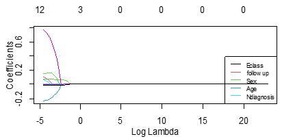
Figure 6. Coefficient plot of LASSO regression
Figure 5 is the mean square error of the estimates, since the Cross-validation $\lambda=0.2999$, the $\log \lambda=-0.523$, which was depicted in Figure 5. Figure 6 shows the coefficient of LASSO regression in line with Table 4. Figure 4 shows that the coefficients of follow-up and sex have been shrunken to zero.
In this investigation, health count data was subjected to modeling by employing a variety of frequentist, Bayesian, and regularized regression models, specifically, ridge and LASSO. Prior to the modeling of the life data, a simulation study encompassing frequentist models such as Poisson, Negative Binomial, Discrete Weibull, and Hurdle Negative Binomial was conducted. Additionally, the simulated data were modeled utilizing Bayesian models including DPMglmm, MCMCglmm, and Bayesian Discrete Weibull.
The findings from the simulation experiment revealed that, in the context of under-dispersed data, ridge regression surpassed LASSO and other frequentist and Bayesian models in terms of the Akaike Information Criterion (AIC). Conversely, based on the Bayesian Information Criterion (BIC), the Dirichlet Prior mixture model demonstrated superior performance. In terms of the Mean Squared Error (MSE), comparable performance between ridge and LASSO was observed, a pattern that manifested in the life data as well.
In conclusion, the outcomes of this study suggest that the superiority of ridge or LASSO in fitting count data is not absolute; instead, it is contingent upon the specific objectives of the study. If model selection is the primary goal, the use of the AIC suggests a preference for ridge regression, although their performance in terms of efficiency, as measured by the mean square error, is largely indistinguishable. Nevertheless, LASSO presents the unique characteristic of shrinking irrelevant variables to zero, thereby emphasizing the significant ones.
The authors hereby acknowledge Covenant University Centre for Research, Innovation and Discovery (CUCRID) for their support toward the completion of this research.
A. Other plots for ridge regression
B. Results of Bayesian discrete Weibull
Posterior estimation for Bayesian discrete Weibull
|
|
Estimate |
Lower |
Upper |
Zero. Included |
|
Int. SEX AGE Ndiag Follow-up Eclass Beta |
0.751743541 -0.040383163 0.002651343 0.973305062 -0.017341374 0.163865080 2.714366416 |
6.501612e-01 -1.080414e-01 -5.818799e-05 9.367946e-01 -1.372259e-01 -2.758960e-01 2.662595e+00 |
0.891886696 0.057647058 0.005475372 1.021458699 0.097705719 0.314701383 2.795901377 |
0 1 1 0 1 1 0 |
Source: Author's computation
[1] Cameron, A.C., Trivedi, P.K. (2005). Microeconometrics Methods and Application. 3rd ed., Cambridge University Press.
[2] Obadina, O.G., Adedotuun, A.F., Odusanya, O.A. (2021). Ridge estimation's effectiveness for multiple linear regression with multicollinearity: An investigation using monte-carlo simulations. Journal of the Nigerian Society of Physical Sciences, 278-281. http://dx.doi.org/10.46481/jnsps.2021.304
[3] Karigowda, R., Nagaraj, P.K. (2022). Off-grid based DOA estimation algorithm using auto-regression (1) Sparse Bayesian Learning with Linear Interpolation Model. Mathematical Modelling of Engineering Problems, 9(5): 1423-1431. https://doi.org/10.18280/mmep.090534
[4] Yendra, R., Hanaish, I.S., Fudholi, A. (2021). Power Bayesian markov chain monte carlo (MCMC) for modelling extreme temperatures in Sumatra Island using generalised extreme value (GEV) and generalised logistic (GLO) distributions. Mathematical Modelling of Engineering Problems, 8(3): 365-376. https://doi.org/10.18280/mmep.080305
[5] Tibshirani, R. (1996). Regression shrinkage and selection via the LASSO. Journal of the Royal Statistical Society Series B (Methodological), 58(1): 267-288. http://dx.doi.org/10.1111/j.2517-6161.1996.tb02080.x
[6] Hoerl, A.E., Kennard, R.W. (1970). Ridge regression: Biased estimation for nonorthogonal problems. Technometrics, 12: 55-67. http://dx.doi.org/10.1080/00401706.1970.10488634
[7] James, G., Witten, D., Hastie, T., Tibshirani, R. (2013). An Introduction to Statistical Learning. New York: springer.
[8] Emmert-Streib, F., Dehmer, M. (2019). High-dimensional LASSO-based computational regression models: regularization, shrinkage, and selection. Mach. Learn. Knowl. Extr., 1(1): 359-383. https://doi.org/10.3390/make1010021
[9] Ateeq, M.K., Sharathchandra, R.G., Meenakshi, R. (2019). Gene prediction in heterogeneous cancer tissues and establishment of least absolute shrinking and selection operator model of lung squamous cell carcinoma. International Journal of Life Science and Pharma Research, 9(4): 34-38.
[10] Amanda, E.C. (2020). Identifying influential variables in the prediction of type 2 diabetes using machine learning methods. Public Health Thesis, Georgia State University. https://scholarworks.gsu.edu/.
[11] Hu, F., Zhang, T. (2020). Study on risk factors of diabetic nephropathy in obese patients with type 2 diabetes mellitus. International Journal of General Medicine, 13: 351-360. https://doi.org/10.2147/IJGM.S255858
[12] Yazdi, M., Golilarz, N.A., Nedjati, A., Adesina, K.E. (2021). An improved lasso regression model for evaluating the efficiency of intervention actions in a system reliability analysis. Neural Comput & Applic, 33: 7913-7928. https://doi.org/10.1007/s00521-020-05537-8
[13] Chintalapudi, N., Angeloni, U., Battineni, G., Di Canio, M., Marotta, C., Rezza, G., Amenta, F. (2022). LASSO regression modeling on prediction of medical terms among seafarers’ health documents using tidy text mining. Bioengineering, 9(3): 124. https://doi.org/10.3390/ bioengineering9030124
[14] Okewole, D.M., Salako, R.J., Adekeye, K.S., Adesanya, S.O. (2022). Regularized regression model for predicting hypertension and type 2 diabetes mellitus in patients. Benin Journal of Statistics, 5: 61-74.
[15] Adedotun A.F., Onasanya O.K., Olusegun O.A., Agboola O.O., Okagbue H.I. (2022). Measure of volatility and its forecasting: Evidence from naira / dollar exchange rate. Mathematical Modelling of Engineering Problems, 9(2): 498-506. https://doi.org/10.18280/mmep.090228
[16] Huttunen, H., Manninen, T., Kauppi, J.P., Tohka, J. (2013). Mind reading with regularized multinomial logistic regression. Machine Vision and Applications, 24(6): 1311-1325. http://dx.doi.org/10.1007/s00138-012-0464-y
[17] Ogoke, U.P., Nduka, E.C., Nja, M.E. (2013). A new logistic ridge regression estimator using exponentiated response function. Journal of Statistical and Econometric Methods, 2(4): 161-171.
[18] Pereira, J.M., Basto, M., da Silva, A.F. (2016). The logistic lasso and ridge regression in predicting corporate failure. Procedia Economics and Finance, 39: 634-641. http://dx.doi.org/10.1016/S2212-5671(16)30310-0
[19] Månsson, K., Shukur, G., Kibria, B.G. (2018). Performance of some ridge regression estimators for the multinomial logit model. Communications in Statistics-Theory and Methods, 47(12): 2795-2804. http://dx.doi.org/10.1080/03610926.2013.784996
[20] Haselimashhadi, H., Vinciotti, V., Yu, K. (2016). A new Bayesian regression model for counts in medicine. arXiv:1601.02820 [stat.ME].
[21] Ismail, N., Zamani, H. (2013). Estimation of claim count data using negative binomial, generalized Poisson, zero-inflated negative binomial and zero-inflated generalized Poisson regression models. In Casualty Actuarial Society E-Forum, 41(20): 1-28.
[22] Jong, P., Heller, G.Z. (2008). Generalized Linear Models for Insurance Data. (1st ed., Cambridge University Press, New York. ISBN-13 978-0-511-38677-0).
[23] Yip, P. (1988). Inference about the mean of a poisson distribution in the presence of a nuisance parameter. Australian Journal of Statistics, 30: 299-306. http://dx.doi.org/10.1111/j.1467-842X.1988.tb00624.x
[24] Adesina, O.S., Olatayo, T.O., Agboola, O.O., Oguntunde, P.E. (2018). Bayesian dirichlet process mixture prior for count data. International Journal of Mechanical Engineering and Technology (IJMET), 9(12): 630-646.
[25] Adedotun, A.F., Adesina, O.S., Onasanya, O.K., Onos, E.S., Onuche, O.G. (2022). CountModels analysis of factors associated with road accidents in Nigeria. International Journal of Safety and Security Engineering, 12(4): 533-542. https://doi.org/10.18280/ijsse.120415
[26] Adedotun, A.F., Olanrewaju, K.O., Abass, I.T., Olumide, S.A., Oluwole, A.O., Onuche, G.O. (2022). Bayesian spatial analysis of socio-demographic factors influencing smoking, use of hard drugs and its residual geographic variation among teenagers of reproductive age in Nigeria. International Journal of Sustainable Development and Planning, 17(1): 277-288. https://doi.org/10.18280/ijsdp.170128
[27] Wang, Z., Ma, S., Zappitelli, M., Parikh, C., Wang, C.Y., Devarajan, P. (2016). Penalized count data regression with application to hospital stay after pediatric cardiac surgery. Statistical Methods in Medical Research, 25(6): 2685-2703. https://doi.org/10.1177/0962280214530608
[28] Noeel, F., Algamal, Z.Y. (2021). Almost unbiased ridge estimator in the count data regression models. Electronic Journal of Applied Statistical Analysis, 14(1): 44-57. https://doi.org/10.1285/i20705948v14n1p44
[29] Rashad, N.K., Hammood, N.M., Algamal, Z.Y. (2021). Generalized ridge estimator in negative binomial regression model. In Journal of Physics: Conference Series, 1897(1): 012019. https://doi.org/10.1088/1742-6596/1897/1/012019
[30] Adesina, O.S., Agunbiade, D.A., Oguntunde, P.E. (2021). Flexible Bayesian Dirichlet mixtures of generalized linear mixed models for count data. Scientific African, 13: e00963. https://doi.org/10.1016/j.sciaf.2021.e00963
[31] R Core Team. (2021). R: A language and environment for statistical computing. R Foundation for Statistical Computing, Vienna, Austria. https://www.R-project.org.
[32] Friedman, J., Hastie, T., Tibshirani, R. (2010). Regularization paths for generalized linear models via coordinate descent. Journal of Statistical Software, 33(1): 1-22. URL https://www.jstatsoft.org/v33/i01/
[33] Wickham, H., François, R., Henry, L., Müller, K. (2022). dplyr: A Grammar of Data Manipulation. R package version 1.0.8. https://CRAN.R-project.org/package=dplyr.
[34] Wickham, H., Averick, M., Bryan, J., Chang, W., McGowan, L.D.A., François, R., Yutani, H. (2019). Welcome to the Tidyverse. Journal of Open Source Software, 4(43): 1686. https://doi.org/10.21105/joss.01686
[35] Veronica Vinciotti. (2016). DWreg: Parametric Regression for Discrete Response. R package version 2.0. https://CRAN.R-project.org/package=DWreg.
[36] Brooks, M.E., Kristensen, K., Van Benthem, K.J., Magnusson, A., Berg, C.W., Nielsen, A., Bolker, B.M. (2017). glmmTMB balances speed and flexibility among packages for zero-inflated generalized linear mixed modeling. The R Journal, 9(2): 378-400. https://journal.r-project.org/archive/2017/RJ-2017-066/index.html.