Rachid El Chaal* | Khalid Hamdane | Moulay Othman Aboutafail
© 2022 IIETA. This article is published by IIETA and is licensed under the CC BY 4.0 license (http://creativecommons.org/licenses/by/4.0/).
OPEN ACCESS
Conducting extensive, time-consuming analysis campaigns is a typical technique to better understand and manage surface water quality. These usually generate a substantial amount of data that is challenging to comprehend. Principal component analysis may be advantageous for such a project (PCA). From the perspective of such an application, eight physico-chemical parameters are important: Sodium (Na+), Bicarbonate (HCO3-), Magnesium (Mg2+), Total Alkalinity (as CaCO3), Chlorides (Cl-), Potassium (K+), Calcium (Ca2+), Sulfates (SO42-), coming from the analysis of 100 water samples collected between February 2014 and December 2015 on 25 stations distributed on Inaouen catchment areas, were analyzed. The principal component analysis applied to the data showed that the variables could be grouped into two principal components. The interpretation of the results using these tools allowed us to understand that the parameters responsible for water quality are related to component Dim1 (HCO3-, CaCO3, K+, Cl-, Na+ and SO42-) and component Dim2 to the processes associated to (Ca2+ and Mg2+) for the physicochemical parameters, the Dim1 factorial design accounts for 67.80% of the variance; it is expressed towards its positive pole by HCO3-, CaCO3, K+, Cl-, Na+ and SO42-, which present good correlations between them. However, the Dim2 factorial plane represents only 17.60%, defined by the Ca2+ and Mg2+ ions towards its positive pole. The Dim1XDim2 plane's typological structure reveals the individualization of three different groupings based on their hydrochemical quality. A feasible reduction in the number of dimensions without a major loss of information was discovered by the PCA. This tool is a good choice from the standpoint of developing management tools.
Eigenvalue, correlations, covariance matrix, multivariate statistical methods, Principal Component Analysis (PCA), statistical processing, water quality, hydrochemical
In Morocco, the situation of the rivers is becoming increasingly worrying because of the essential quantities of untreated; polluting discharges poured into these aquatic ecosystems [1]. To study this situation closely, we chose the Inaouen catchment area, which is experiencing growing demography and continuous development of the industrial sector along its banks. This work represents the first study carried out on this hydrosystem. It aims to evaluate the impact of discharges on the quality of water resources through a physicochemical characterization [2]. To highlight the global quality of water and its Spatio-temporal evolution in the studied watercourses [3], we considered it interesting to make a synthesis of these results by the statistical method (principal component analysis PCA) [4].
We attempted to demonstrate that the principal component analysis (PCA) method could be a tool allowing us to specify with objectivity the state and quality of these waters. The study's objectives are to: evaluate the physicochemical quality of surface waters; and monitor the spatial evolution of the studied variables based on seasonal analytical monitoring of 25 stations distributed along the Inaouen watershed and its main tributaries [5-8]. In this study, we thus endeavored to show, on this medium, that the typology of the stations was related, on the one hand, to the physical or chemical characteristics of the surrounding environments and, on the other hand, to the degradation of the quality of the surface waters of the Inaouen catchment area, under the effect of the anthropic activity [3, 9].
Using PCA for data interpretation in this context seems like an intriguing solution to better understand water quality and the biological health of the ecosystems studied [10-13]. This method also has the benefit of identifying and connecting the many causes (sources) to the consequences on the seen aquatic systems [5-8]. Consequently, it is a better tool for managing water resources, enabling quick fixes for contamination issues [14].
It is in this context that the present study is conducted. It is based on using multivariate statistical analysis techniques, namely Principal Component Analysis (PCA), to understand the processes that govern surface water in the region.
2.1 Environment and study site
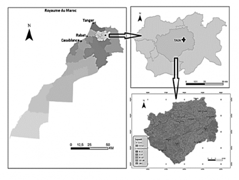
The study is only conducted in the Oued Inaouen watershed, which has a total measured area of 3,396 km2 and is located upstream of the Idriss I dam (Figure 1) [15]. The Sebou basin upstream of the Idriss I dam makes up 8.3% of the total area. Its boundaries are the Upper Sebou in the south, the Upper Ouergha in the north, and the Middle Mouloya watershed in the east. On the right bank of this basin, it primarily drains the marly formations of the Pre-Rifain relief. On the left bank, it primarily drains the carbonate formations of the Middle Atlas Causse. The Oued Inaouen receives the Oued Flows of Amlil, Larbaa, and Lahdar on its right bank. These tributaries gather the runoff from the pre-rific hills. On its left bank, the Oued Inaouen receives tributaries from the Middle Atlas limestones Matmata, Zerg, Bouzemlane, and Bouhlou, which are often karstic in this area and are partly fed by the Tazekka central massif. Fifty-two wastewater discharges from the city of Taza are spread. There could be up to 5,000,000 m3 of wastewater released into waterways each year. Given the population growth in the city of Taza, this flow is increasing year over year [3].
Figure 1. Geographical location of the study area
2.2 Samples
The sampling campaigns were carried out mainly on fixed dates throughout the study period from February 2014 to December 2015. The frequency of measurement is seasonal (spring, summer, autumn and winter) to obtain a reasonably representative picture of water quality and its seasonal, annual and multi-year evolution [16].
Our database contains 100 surface water samples (observations) collected in the province of Taza; water samples were collected, transported, and stored according to the National Drinking Water Office's (ONEP) policy and procedures [17]. A portion of the analysis was done there. Another portion was done at the Regional University Centre of Interface (CURI) attached to the Sidi Mohamed Ben Abdellah University (USMBA) of Fez at the time of sampling to avoid the change and temperature, conductivity, pH using a multi-parameter analyzer Type CONSORT - Model C535, and dissolved oxygen by the titration method of Winkler. The methods used at CURI Laboratory: volumetry for bicarbonates, chlorides, calcium and magnesium; molecular absorption spectrophotometry for sulfates, nitrates, nitrites, ammonium ions and orthophosphates; and flame spectrophotometry for sodium and potassium. The four heavy metals are analyzed by atomic absorption spectrum (AAS).
2.3 Physicochemical variables studied
The variables retained for this statistical study are the eight major ions: Sodium (Na+), Bicarbonate (HCO3-), Magnesium (Mg2+), Chlorides (Cl-), Potassium (K+), Calcium (Ca2+), Sulfates (SO42-) and Total Alkalinity (as CaCO3). The means and standard deviations of these studied parameters are reported in the Table 1.
Table 1. The statistical summary of data
|
Parameter |
Number of data |
Mean |
Median |
Minimum |
Maximum |
Variance |
Standard deviation |
|
HCO3- |
100 |
80,63 |
57,95 |
3,66 |
634,40 |
7788,82 |
88,25 |
|
CaCO3 |
100 |
66,09 |
47,50 |
3,00 |
520,00 |
5233,01 |
72,34 |
|
Mg2+ |
100 |
3,17 |
2,05 |
0,20 |
25,00 |
14,48 |
3,81 |
|
Na+ |
100 |
24,51 |
5,40 |
1,00 |
540,00 |
4197,42 |
64,79 |
|
K+ |
100 |
1,72 |
0,97 |
0,10 |
13,00 |
4,43 |
2,10 |
|
Cl- |
100 |
25,84 |
2,45 |
0,40 |
550,00 |
5676,23 |
75,34 |
|
Ca2+ |
100 |
17,79 |
15,00 |
1,00 |
110,00 |
316,65 |
17,79 |
|
SO42- |
100 |
7,83 |
5,00 |
0,28 |
150,00 |
244,37 |
15,63 |
2.4 Data standardization
Variables in the principal component analysis are frequently normalized [18, 19]. This is especially advised when the variables are measured in various units (such as kilograms, kilometres, centimetres, etc.); otherwise, the PCA result will be significantly impacted.
Making the variables similar is the goal. The variables are often normalized to have a mean of zero, a standard deviation of one, and a standard deviation of one [20, 21].
Technically speaking, the method entails converting the data by subtracting a reference value (the variable's mean) from each value and dividing the result by the standard deviation. The data left over after this transformation is referred to as centred-reduced data. Normalized PCA is the name of the PCA used to analyze these modified data [22].
Before PCA and clustering studies, data normalization was widely utilized in gene expression data analysis.
The information can be altered as follows after normalizing the variables [23]: $\frac{x_i-\operatorname{mean}(x)}{s d(x)}$.
Where mean(x) is the average of the values of x, and sd(x) is the standard deviation.
2.5 Statistical processing of data
As a multidimensional descriptive statistical technique, Principal Component Analysis (PCA) enables the analysis and presentation of a data set containing individuals characterized by quantitative variables [24, 25]. A statistical approach that allows the investigation of multivariate data is this one (data with several variables). It is possible to think of each variable as a different dimension [26]. It could be very challenging to show your dataset in a multidimensional hyperspace if it has more than three variables. The crucial data in a multivariate data table are extracted and visualized using principal component analysis [27]. This data is combined via PCA into a small number of new variables called principal components. The original variables are linearly combined to create these new variables [28]. There are fewer or the same number of principal components as there were original variables. The total variance or inertia of a data set is the information it holds [29]. The goal of PCA is to find the principal axes or principal components [30], otherwise known as the directions along which the data vary most. In other words, PCA preserves as much information as possible while condensing the dimensions of multivariate data to two or three principal components that can be graphically represented [31]. Giving a graphical representation of the data and the relationships between the variables is challenging when there are many observed variables [32].
The most important parameters that describe the quality of surface waters and illustrate their variability can be found using this method, which has been widely used to interpret hydrochemical data of hydro systems. Principal component analysis was the foundation for the statistical analysis.
R software (version 3.6.3) was used to generate the intermediate correlation matrix and project the variables into the space of the Dim1 and Dim2 axes.
2.6 PCA procedure
PCA replaces a family of variables with new variables called principal components (PC) [33-35]. The latter is of maximum variance and uncorrelated two by two. They are linear combinations of the original variables. Let us consider a set of data collected during a normal operation of the system under study. A matrix can represent these data [36].
$\mathbf{X}=[\mathbf{x}(1), \cdots, \mathbf{x}(N)]^T \in \mathbb{R}^{N \times m}$ (1)
where, $N$ is the number of observations and $m$ is the number of measured variables. Each row of the data matrix $\mathbf{X}$ represents an observation in the form of a vector of measurements collected at a time $k$ generally centred [37].
$\mathbf{x}(k)=\left[x_1(k), \cdots, x_m(k)\right]^T \in \mathbb{R}^m$ (2)
where, $x_j(k)$ with $j=\{1, \cdots, \mathrm{m}\}$ represents the measurement of the variable $j$ at time $k$. By definition, the covariance matrix is given in the research [37]:
$\Sigma=\mathbb{E}\left\{\mathbf{x} \mathbf{x}^T\right\}=\frac{1}{N} \mathbf{X}^T \mathbf{X} \in \mathbb{R}^{m \times m}$ (3)
According to the principle of PCA, it is assumed that a vector of components $\hat{\mathbf{t}} \in \mathbb{R}^{\ell}$ is associated with each observation vector whose representation it optimizes in the sense of minimizing the estimation error of $x$ or the maximization of the variance of $\hat{\mathbf{t}}$. At each time $k$, the vectors $\hat{\mathbf{t}}$ and $\mathbf{x}$ are linked by a linear transformation of type $\hat{\mathbf{t}}(k)=$ $\hat{P}^T \mathbf{x}(k)$ such that the transformation matrix $\hat{P} \in \mathbb{R}^{m \times \ell}$ verifies the orthogonality condition $\hat{P}^T \hat{P}=\mathbf{I}_{\ell} \in \mathbb{R}^{\ell \times \ell}$.
The columns of the matrix $\hat{P}$ are the vectors of an orthonormal basis of a subspace $\mathbb{R}^{\ell}$ of reduced representation of the original data. The linear transformation results in the projection of the original data expressed in the space of dimension $m$ to an orthogonal subspace of dimension $\ell$. The components $t_j(k)$ with $j=\{1, \cdots, \ell\}$ of the vector $\hat{\mathbf{t}}(k)$ are the projections of the elements of the data vector $\boldsymbol{x}(k)$ in the subspace $\mathbb{R}^{\ell}$.
The representation optimization based on the projection matrix $\hat{P}$ is obtained by minimizing the squared estimation error $o \mathbf{x}$ f. Let us note by $\hat{P}$ the optimal representation matrix, which can be given in study [37]:
$\hat{P}=\arg \min _{\grave{P}}\left\{J_e(\grave{P})\right\}$ (4)
where, $J_e$ is the criterion for the estimation error by PCA, which should be minimized [38]. Under the Orthogonality constraint of the projection matrix $\hat{P}$ We can write [39]:
$\begin{aligned} J_e(\hat{P}) & =\mathbb{E}\left\{\|\mathbf{x}-\hat{\mathbf{x}}\|^2\right\}=\mathbb{E}\left\{\left\|\mathbf{x}-\hat{P} \hat{P}^T \mathbf{x}\right\|^2\right\} \\ & =\mathbb{E}\left\{(\mathbf{x}-\hat{P} \hat{\mathbf{t}})^T(\mathbf{x}-\hat{P} \hat{\mathbf{t}})\right\}=\mathbb{E}\left\{\mathbf{x}^T \mathbf{x}-\hat{\mathbf{t}}^T \hat{\mathbf{t}}\right\} \\ & =\mathbb{E}\left\{\operatorname{tr}\left(\mathbf{x x}^T\right)-\hat{\mathbf{t}}^T \hat{\mathbf{t}}\right\}=\operatorname{tr}\{\Sigma\}-\mathbb{E}\left\{\hat{\mathbf{t}}^T \hat{\mathbf{t}}\right\} \\ & =\operatorname{tr}\{\Sigma\}-J_v(\hat{P})\end{aligned}$ (5)
where, $\operatorname{tr}\{$. denotes the trace of a square matrix. Since the term $\operatorname{tr}\{\Sigma\}$ is a constant, minimizing the criterion $J_e$ is the same as maximizing the $J_v$ Given by [39]:
$\begin{aligned} J_v(\hat{P})=\mathbb{E}\left\{\hat{\mathbf{t}}^T \hat{\mathbf{t}}\right\} & =\mathbb{E}\left\{\sum_{j=1}^{\ell} t_j^2\right\}=\sum_{j=1}^{\ell} \mathbb{E}\left\{t_j^2\right\} \\ = & \sum_{j=1}^{\ell} \operatorname{Var}\left\{t_j\right\}\end{aligned}$ (6)
From the previous equation, maximizing the $J_v$ equivalent to maximizing the variance of the $t_j$. Thus, the optimization problem is reformulated as follows [37]:
$\hat{\boldsymbol{P}}=\arg \min _{\hat{P}}\left\{J_e(\hat{P})\right\}=\arg \max _{\hat{P}}\left\{J_v(\hat{P})\right\}$ (7)
To determine the column vectors of the matrix $\hat{P}$, we note by $t \in \mathbb{R}$ the projection of the data vector $\mathbf{x}$ along a direction represented by a unit vector $p \in \mathbb{R}^m$. The scalar product $t=$ $\mathbf{x}^T p=p^T \mathbf{x}, \mathbf{x}$ obtains the component $\mathrm{t}$ under the constraint $\|p\|^2=p^T p=1$. In particular, it represents a new variable with a mean and a variance that depend on the statistical properties of $\mathbf{x}$ as follows [39-41]:
$\mathbb{E}\{t\}=\mathbb{E}\left\{p^T \mathbf{x}\right\}=p^T \mathbb{E}\{\mathbf{x}\}=0$ (8)
$\begin{aligned} \operatorname{Var}\{t\} & =\mathbb{E}\left\{(t-\mathbb{E}\{t\})^2\right\}=\mathbb{E}\left\{t^2\right\} \\ & =\mathbb{E}\left\{\left(p^T \mathbf{x}\right)\left(\mathbf{x}^T p\right)\right\}=p^T \mathbb{E}\left\{\mathbf{x x}^T\right\} p \\ & =p^T \Sigma p\end{aligned}$ (9)
The maximization of the projection variance, under the condition of a unit norm of the vector p, represents an equality-constrained optimization problem that the Lagrange function can formalize [40-43]:
$\mathcal{L}(p, \lambda)=J_v(p)-\lambda\left(p^T p-1\right)$ $=p^T \Sigma p-\lambda\left(p^T p-1\right)$ (10)
where, $\lambda \in \mathbb{R}$ is the Lagrange multiplier. Taking into account the symmetry of the matrix $\Sigma$, the vector $p$ maximizes the optimization criterion $J_v$ is a solution of the following system of equations [37]:
$\left\{\begin{array}{l}\partial \mathcal{L}(p, \lambda) / \partial p=\Sigma p-\lambda p=0 \\ \partial \mathcal{L}(p, \lambda) / \partial \lambda=p^T p-1=0\end{array}\right.$ (11)
Consequently, the solution of this system of equations is identified as a problem of estimating normalized eigenvalues and eigenvectors of the matrix $\Sigma$. Such a system of equations admits real solutions of the variables $\lambda$ obtained by solving the following characteristic equation [41]:
$\operatorname{Det}\left\{\Sigma-\lambda \mathbf{I}_m\right\}=0$ (12)
where, Det $\{$.$\} is the determinant of a square matrix. \mathbf{I}_m$ is the identity matrix of order $m$. The solutions of the previous equation represent the eigenvalues of $\Sigma$. To each eigenvalue, $\lambda$ is associated with an eigenvector $p$ verifying $\left(\Sigma-\lambda \mathbf{I}_m\right) p=0$.
This allows us to have $m$ eigenvectors $\mathbf{p}_i$ associated with the $m$ eigenvalues $\lambda_i$ of the matrix $\Sigma$, thus verifying the relation $\Sigma \mathbf{p}_i=\lambda_i \mathbf{p}_i$ with $i=\{1, \cdots, m\}$. In matrix form, such a relationship leads to writing the following [37, 44, 45]:
$\Sigma \mathbf{P}=\mathbf{P B}$ (13)
$\mathbf{P}=\left[\mathbf{p}_1, \cdots, \mathbf{p}_m\right] \in \mathbb{R}^{m \times m}$ represents the data projection matrix. It is orthonormal since its columns correspond to the eigenvectors of $\Sigma$:
$\mathbf{P}^T \mathbf{P}=\mathbf{P P}^T=\mathbf{I}_m \in \mathbb{R}^{m \times m}$ (14)
$\mathbf{B}=\operatorname{diag}\left\{\lambda_1, \cdots, \lambda_m\right\} \in \mathbb{R}^{m \times m}$ represents the diagonal matrix consisting of the diagonal elements of the eigenvalues of $\Sigma$.
From Eqns. (13) and (14), we can deduce that $\mathbf{P}^T \Sigma \mathbf{P}=\mathbf{B}$. This allows us to conclude that the first direction, having a maximum projection variance of $\mathbf{x}$, is carried by the eigenvector $\mathbf{p}_1$ associated with the largest eigenvalue $\lambda_1$. The latter represents the variance of such a direction. The second factorial axis also renders the maximum variance while orthogonal to the first. Its variance $\lambda_2$ is less important than that corresponding to the first direction. Therefore, the diagonal elements of $\mathbf{B}$ are arranged in descending order [46-49]: $\lambda_1 \geq \cdots \geq \lambda_m$
Considering the matrix $\mathbf{P}$, the data vector $\boldsymbol{x}(k)$ can be transformed without any loss of information into a vector of principal components (PC) [36, 37, 39]:
$\mathbf{t}(k)=\left[t_1(k), \cdots, t_m(k)\right]^T=\mathbf{P}^T \mathbf{x}(k) \in \mathbb{R}^m$ (15)
where, the $\mathrm{CP} t_j$ with $j=\{1, \cdots, m\}$ is defined by:
$t_j(k)=\mathbf{p}_j^T \mathbf{x}(k)=\mathbf{x}^T(k) \mathbf{p}_j$ (16)
These are statistically uncorrelated [37, 39]:
$\mathbb{E}\left\{t_i t_j\right\}=\mathbb{E}\left\{\mathbf{p}_i^T \mathbf{x x}^T \mathbf{p}_j\right\}=\mathbf{p}_i^T \Sigma \mathbf{p}_j=0 i \neq j$ (17)
The notation in matrix form allows us to define the matrix of CP as follows [40, 41]:
$\mathbf{T}=[\mathbf{t}(1), \cdots, \mathbf{t}(N)]^T=\mathbf{X P} \in \mathbb{R}^{N \times m}$ (18)
The determination of the data vector $x(k)$ à from the associated vector of CP $\mathbf{t}(k)$ is given by:
$\mathbf{x}(k)=\operatorname{Pt}(k)=\sum_{j=1}^m \mathbf{p}_j t_j(k)$ (19)
The data reduction is performed through the $\ell$ first $\mathrm{CP}$ with the largest variances. As a result, the $\ell$ first eigenvectors form the reduced vector subspace for the initial data. The estimation of $\hat{\mathbf{x}}(k)$ of the data vector $\boldsymbol{x}(k)$ in this reduced subspace (often called representation or principal subspace and denoted $\hat{S})$ is given by references [40, 42, 43, 50]:
$\hat{\mathbf{x}}(k)=\hat{\mathbf{P}} \hat{\mathbf{t}}(k)=\hat{\mathbf{P}} \hat{\mathbf{P}}^T \mathbf{x}(k)=\hat{\mathbf{C}} \mathbf{x}(k)$ (20)
where, the optimal representation matrix expressed in Eq. (7) is defined as follows:
$\hat{\mathbf{P}}=\left[\mathbf{p}_1, \cdots, \mathbf{p}_{\ell}\right] \in \mathbb{R}^{m \times \ell}$ (21)
$\hat{\mathbf{t}}(k)=\hat{\mathbf{P}}^T \mathbf{x}(k) \in \mathbb{R}^{\ell}$ represents the vector of the $\ell$ first $C P$. The matrix $\hat{\mathbf{C}} \in \mathbb{R}^{m \times m}$ thus characterizes the PCA model.
However, dimension reduction usually results in a loss of information that is recovered in a residual vector $\tilde{\mathbf{x}}(k)$. The latter is expressed in a residual subspace $\tilde{\mathcal{S}}$ consisting of the remainder of the CPs associated with the $(m-\ell)$ last eigenvectors [37, 39, 41]:
$\tilde{\mathbf{x}}(k)=\tilde{\mathbf{P}} \tilde{\mathbf{t}}(k)=\tilde{\mathbf{P}} \tilde{\mathbf{P}}^T \mathbf{x}(k)=\tilde{\mathbf{C}} \mathbf{x}(k)$ (22)
with
$\tilde{\mathbf{P}}=\left[\mathbf{p}_{\ell+1}, \cdots, \mathbf{p}_m\right] \in \mathbb{R}^{m \times(m-\ell)}$ (23)
and
$\tilde{\mathbf{C}}=\tilde{\mathbf{P}} \tilde{\mathbf{P}}^T=\mathbf{I}_m-\hat{\mathbf{C}}$ (24)
The matrix $\tilde{\mathbf{C}} \in \mathbb{R}^{m \times m}$ Describes the residual model. We can see here that PCA is a modelling approach that allows us to obtain a PCA model of a studied system.
The interpretation of the principle of PCA modelling represents a partitioning of the space $\mathbb{R}^m$ of measurements $\mathbf{x}(k)$ into the main subspace $\hat{\mathcal{S}}$ and a residual subspace $\tilde{\mathcal{S}}$. Therefore, the vector of measures $\mathbf{x}(k)$ is decomposed as follows:
$\mathbf{x}(k)=\hat{\mathbf{x}}(k)+\tilde{\mathbf{x}}(k)$ (25)
In particular, a geometric property of orthogonality between the estimated and the residual vector is always verified since [39, 41, 42]:
$\tilde{\mathbf{C}} \hat{\mathbf{C}}=\hat{\mathbf{C}} \tilde{\mathbf{C}}=\mathbf{0}_m \in \mathbb{R}^{m \times m}$ (26)
This implies that the principal subspace and the residual subspace are orthogonal for all values of $\ell$, thus [37, 40, 43],
$\tilde{\mathbf{x}}^T(k) \hat{\mathbf{x}}(k)=0$ (27)
3.1 Statistical analysis of results
3.1.1 Correlations between variables
A data matrix with eight variables and 100 samples was used to analyze the physicochemical data (8 variables and 100 individuals). The data was processed using the R program.
The strength of the relationships between the parameters analyzed can be determined by examining the bivariate linear correlations between them. Table 2 contains the correlation matrix for the eight parameters measured throughout our investigation. Because the sampling stations were pooled to construct this matrix, care must be taken when interpreting the correlation coefficients. Indeed, both spatial and temporal changes impact them at once. Interesting correlations are found in this table's significant Pearson correlation coefficients, which are highlighted in bold. This expresses the notion of a linear link between two variables that contradicts their independence. It is a common tool to describe simple relationships without worrying about cause and effect.
Consequently, there is a significant positive association between HCO3 and the following variables: CaCO3 (0.97), Na (0.80), K (0.72) and SO4 (0,75). Strong and positive correlations are observed between CaCO3 and the minerals Na, SO4 and K (R between 0.73 and 0.80) are seen between CaCO3 and the minerals Na, SO4 and K, as well as with Mg and Cl. It's also noteworthy to note how Mg and Na frequently correlate with the variables K, Cl, Ca, and SO4.
3.1.2 PCA results
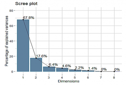
We carried out the statistical tests that permit PCA because its usage must always be justified. A score of 2748.85 for the Chi-square was obtained using Bartlett's sphericity test (with a degree of freedom of 378 and a significance level of p (p$\prec$0.0005), proving that the variables are substantially correlated to permit a reduction in the dimension. In a subsequent phase, we assessed the sampling's suitability concerning the viability of PCA using the Kaiser-Meyer-Olkin approach (KMO index). This acceptable adequacy is confirmed by the value obtained (0.816), which tends toward 1. The variance accumulation test, also known as the Scree test, in a PCA determines the number of components to be extracted. Component extraction should halt when the slope of the eigenvalue graph changes. The extracted dimensions' interpretability must be considered while deciding how many components to extract. The eigenvalue graph produced during this study is shown in Figure 2.
Figure 2. Graphical representation of calculated variance percentages
Table 2. The correlation matrix of the eight measured parameters
|
HCO3 |
CaCO3 |
Mg |
Na |
K |
Cl |
Ca |
SO4 |
|
|
HCO3 |
1,00 |
|||||||
|
CaCO3 |
0,97 |
1,00 |
||||||
|
Mg |
0,59 |
0,59 |
1,00 |
|||||
|
Na |
0,80 |
0,80 |
0,38 |
1,00 |
||||
|
K |
0,72 |
0,77 |
0,56 |
0,82 |
1,00 |
|||
|
Cl |
0,61 |
0,65 |
0,54 |
0,91 |
0,75 |
1,00 |
||
|
Ca |
0,48 |
0,41 |
0,74 |
0,10 |
0,22 |
0,28 |
1,00 |
|
|
SO4 |
0,75 |
0,73 |
0,33 |
0,85 |
0,64 |
0,76 |
0,14 |
1,00 |
Table 3. Eigenvalues and percentages expressed by the principal axes
|
Dimensions (factor) |
Eigenvalue |
Variance percent |
Cumulative eigenvalue |
Cumulative variance percent |
|
1 |
5.422 |
67.8 |
5.422 |
67.80 |
|
2 |
1.410 |
17.6 |
6.832 |
85.40 |
|
3 |
0.510 |
6.4 |
7.342 |
91.80 |
|
4 |
0.371 |
4.6 |
7.713 |
96.40 |
|
5 |
0.172 |
2.2 |
7.885 |
98.60 |
|
6 |
0.112 |
1.4 |
7.997 |
100 |
|
7 |
0.003 |
00 |
8.00 |
100 |
3.1.3 Analysis in the space of the variables of the factorial plane Dim1xDim2
After PCA, the number of principal axes to keep can be calculated using eigenvalues according to the Kaiser criterion which states that when normalizing the data, a principal component (PC) with an eigenvalue greater than one is said to reflect more variation than a single original variable. This serves as a typical cut-off point for keeping PCs. Keep in mind that this only works if the data is standardized
Sadly, there isn't a widely used objective approach for determining how many principal axes are enough. It will rely on the specific data set and application domain. In real-world situations, it is common to focus on the first few principal axes while looking for noteworthy data patterns. Our analysis's first two principal components account for 85.40% of the variation. This % is suitable.
Examining the eigenvalue plot provides another way to count the principal components (called the scree plot). Beyond which the remaining eigenvalues are all very modest and similar in size, the number of axes is determined.
Analyzing the numerical outcomes of this PCA reveals that the Dim1 axis accounts for more than half (i.e., 67.8%) of the total variance of the data, according to the eigenvalues (Figure 2 and Table 3). 17.6% of the overall variation in the data is explained by the Dim2 axis. As a result, the Dim1XDim2 factorial design extracts 85.40% of the variability from the data table. As a result, just these first two axes will be used to analyze the PCA findings.
The initial variables are more or less associated with them and are combined linearly to get the principal components. The starting variables are projected to account for the most information in the reduced dimension space defined by these components. The correlation coefficient values between the variables and the two components are displayed in Table 4. The correlations that best describe each component and are, therefore, the most significant are shown in bold.
Table 4. Correlation coefficients between the variables and the first two components
|
|
Dim1 |
Dim2 |
|
HCO3 |
0.924 |
0.056 |
|
CaCO3 |
0.932 |
0.051 |
|
Mg |
0.682 |
0.618 |
|
Na |
0.905 |
-0.385 |
|
K |
0.868 |
-0.136 |
|
Cl |
0.863 |
-0.179 |
|
Ca |
0.456 |
0.837 |
|
SO4 |
0.831 |
-0.345 |
Table 5. Contributions of variables (%)
|
|
Dim1 |
Dim2 |
|
HCO3 |
16.026 |
0.227 |
|
CaCO3 |
16.019 |
0.216 |
|
Mg |
8.582 |
27.155 |
|
Na |
15.132 |
10.548 |
|
K |
13.897 |
1.317 |
|
Cl |
13.739 |
2.297 |
|
Ca |
3.846 |
49.765 |
|
SO4 |
12.750 |
8.460 |
Figure 3. Graphical representation of the contributions of variables to the first five principal axes
Contributions of variables to the principal axes
We will pay close attention to variables that strongly influence the factorial axis in either a positive or negative way, making it easier to comprehend the reason for the variability the axes explain (Table 5).
A bar plot of the variables contributing most to the principal components Dim1 and Dim2 (Figures 3 and 4):
(a) For Dim1
(b) For Dim2
Figure 4. Graphical representation to highlight the most contributing variables for the first two principal axes
The red dotted line represents the expected average contribution in the graph above. The expected value would be 1/length(variables), which would equal 1/8, or 12.5% if the contribution of the variables were uniform. A variable that contributes more than this threshold to a specific component may be regarded as relevant for the component.
The variables HCO3, CaCO3, Na, K, Cl, and SO4 then contribute to the principal component Dim1, which means that they strongly attract the Dim1 axis in that direction and help to build that axis.
Additionally, the factors Mg and Ca help to form the principal component Dim2. They are therefore in charge of its creation and definition.
Figure 5. Graph of the contributions of the variables on the factorial plane Dim1xDim2
The correlation graph (Figure 5) highlights the most significant (or contributing) variables:
Quality of representation of the variables:
The quality of representation of the variables on the PCA map is called cos² (cosine squared).
Table 6. Value of the square cosines
|
|
Dim1 |
Dim2 |
|
HCO3 |
0.868 |
0.003 |
|
CaCO3 |
0.862 |
0.003 |
|
Mg |
0.465 |
0.382 |
|
Na |
0.820 |
0.148 |
|
K |
0.753 |
0.018 |
|
Cl |
0.744 |
0.032 |
|
Ca |
0.208 |
0.701 |
|
SO4 |
0.691 |
0.119 |
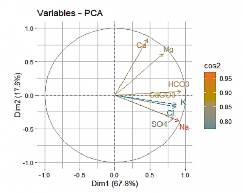
The high cos² of the variables HCO3, CaCO3, Na, K, Cl and SO4and of the variables Mg and Ca indicate a good representation of the variables on the main axis Dim1 and the main axis Dim2 (Figure 6 and Table 6), respectively. In this case, they are positioned near the circumference of the correlation circle. They are more important to interpret these two principal components.
Figure 6. Graphical representation to highlight the variables with a good representation on the first five principal axes
The correlation graph (Figure 7) can be used to emphasize the most significant (or contributing) variables:
Figure 7. Plot of cos² values of variables on the factorial plane Dim1 and Dim2
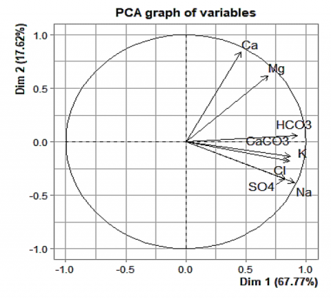
The correlation circle (Figure 8):
The quality of the variables' representation is measured by the distance between the variables and the origin. The variables HCO3, CaCO3, Na, Mg, Ca and SO4 are far from the origin, so they are well represented by the PCA. The correlation circle shows that the eight variables considered in the PCA contribute to the definition of the Dim1 x Dim2 factorial design.
The Dim1 component accounting for 67.8% of the variances is essentially made up of the mineral variables positively structuring the Dim1 component: HCO3, CaCO3, Na, K, Cl and SO4(which contribute with 87.53% to the formation of the Dim1 component), translating the alkalinity of the water and generally describing the mineralization of the water. The Dim1 component can be linked here to the notion of the trophic potential of waters.
The Dim2 component (17.60% of the variance) is constituted in its positive part by the variables Mg and Ca, which contribute with 76.92% to the formation of the component Dim2; these two variables structure the Dim2 component positively and generally describe the hardness of the water, whereas the Dim2 component is characterized by waters coming from the alteration of the mother rock.
Figure 8. Correlation plot of variables on the Dim1 and Dim2 factorial plane
3.1.4 Projection of individuals in the Dim1XDim2 factorial plane
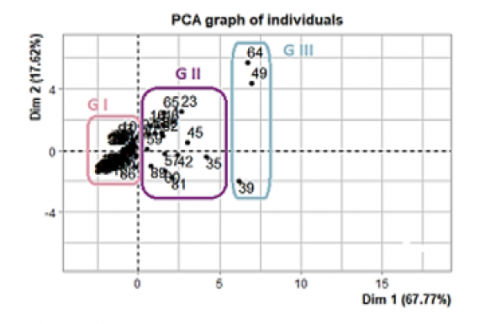
The sampling stations in the reconstructed planes of the Dim1 and Dim2 components are shown in Figure 9. The sample stations are divided into three major groupings, as may be seen from this illustration. Group G III, which includes stations 39, 49, and 64 in the positive half of component 1, and group G II, which includes a number of stations (23, 35, 42, 45, 65....). Most of the stations in group G I are found in component Dim2's negative portion.
Based on the factorial map Dim1 x Dim2 (Figure 9 and Figure 10), the PCA results show that the different stations are positioned (on Dim1) according to the mineralization and alkalinity of their waters. Thus, the least mineralized study stations are located on the negative side of the Dim2 component (G I). also, the stations with a medium or low hardness are located in the negative part of the Dim2 component (G I) and the positive part of the Dim2 component (G II).
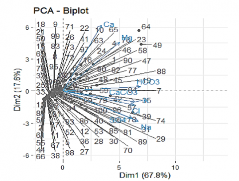
Group G III is characterized by high Mg and Ca contents (because the springs are on the same side of the variable). This reflects the hardness of these sources. While the group G II is medium rich in HCO3, CaCO3, Na, K, Cl and SO4 illustrate important mineralization. Let us finally point out that all the stations of the G I group positioned on the negative side of the Dim2 component are less mineralized than those of G II and G III (because their sources are on the opposite side of the variables), see Biplot (Figure 10).
Figure 9. Representation of the sampling stations on the Dim1XDim2 factorial plane
Figure 10. Biplot of sampling stations and variables on the Dim 1XDim2 factorial plane
The principal component analysis carried out on a data matrix comprising 8 physicochemical variables allowed us to identify two main axes which summarize the main information of this matrix: The Dim1 axis, which can be assimilated to an axis translating a gradient of mineralization and alkalinity and the Dim2 axis which would translate the degree of hardness. Similarly, the stations are well typed and therefore well-structured by their physicochemical data.
At the end of this PCA analysis, we can say that the stations are well typed and thus well-structured by their physicochemical data: A two-dimensional space was sufficient to summarize most of the information concerning the variability present in the initial 8-dimensional space.
Through this analysis, we have highlighted major trends in the data, such as groupings of individuals or oppositions between individuals or between variables (reflecting that the variables are inversely correlated). The graphical representations provided by PCA are simple and informative. The PCA can be the first analysis for the hydrochemical study whose results will be enriched by another factorial analysis or an automatic data classification.
[1] Bahhou, J., Mhamdi, M.A. (1999). Diet changes in the biochemical composition of the phytoplankton in the Idriss first reservoir (Fes, Morocco). Journal de Chimie Physique et de Physico-Chimie Biologique, 96: 339-351. https:/doi.org/10.1051/jcp:1999141
[2] Xu, S.G., Cui, Y.X., Yang, C.X., Wei, S.J., Dong, W.P., Huang, L.H. (2021). The fuzzy comprehensive evaluation (FCE) and the principal component analysis (PCA) model simulation and its applications in water quality assessment of Nansi Lake Basin, China. Environmental Engineering Research, 26(2): 200022. https://doi.org/10.4491/eer.2020.022
[3] Rezouki, S., Allali, A., Najat, T., Eloutassi, N., Fadli, M. (2021). Spatio-temporal evolution of the physico-chemical parameters of the Inaouen wadi and its tributaries. Moroccan Journal of Chemistry, 9(3): 576-587. https:/doi.org/10.48317/IMIST.PRSM/morjchem-v9i3.23521
[4] Mutlu, E., Arslan, N., Tokatli, C. (2021). water quality assessment of yassialan dam lake (karadeniz region, turkey) by using principal component analysis and water quality index. Acta Scientiarum Polonorum-Formatio Circumiectus, 20: 55-65. https://doi.org/10.15576/ASP.FC/2021.20.2.55
[5] Zavareh, M., Maggioni, V., Sokolov, V. (2021). Investigating water quality data using principal component analysis and granger causality. Water, 13(3): 343. https://doi.org/10.3390/w13030343
[6] Zeng, W.B., Wan, X.M., Wang, L.Q., Lei, M., Chen, T.B., Gu, G.Q. (2022). Apportionment and location of heavy metal(loid)s pollution sources for soil and dust using the combination of principal component analysis, Geodetector, and multiple linear regression of distance. Journal of Hazardous Materials, 438: 129468. https:/doi.org/10.1016/j.jhazmat.2022.129468
[7] Fatima, S.U., Khan, M.A., Siddiqui, F., Mahmood, N., Salman, N., Alamgir, A. (2022). Geospatial assessment of water quality using principal components analysis (PCA) and water quality index (WQI) in Basho Valley, Gilgit Baltistan (Northern Areas of Pakistan). Environmental Monitoring and Assessment, 194: 151. https:/doi.org/10.1007/s10661-022-09845-5
[8] Chauhan, N., Paliwal, R., Kumar, V., Kumar, S., Kumar, R. (2022). Watershed prioritization in Lower Shivaliks Region of India using integrated principal component and hierarchical cluster analysis techniques: A case of upper Ghaggar Watershed. Journal of the Indian Society of Remote Sensing, 50: 1051-70. https://doi.org/10.1007/s12524-022-01519-6
[9] AlaouiMhamdi, M., Aleya, L., Bahhou, J. (1996). Nitrogen compounds and phosphate of the Driss I reservoir (Morocco): Input, output and sedimentation. Hydrobiologia, 335: 75-82. https://doi.org/10.1007/BF00013685
[10] Arora, S., Keshari, A.K. (2021). Pattern recognition of water quality variance in Yamuna River (India) using hierarchical agglomerative cluster and principal component analyses. Environmental Monitoring and Assessment, 193: 494. https://doi.org/10.1007/s10661-021-09318-1
[11] Gong, M.Y., Miller, C., Scott, M., O’Donnell, R., Simis, S., Groom, S. (2021). State space functional principal component analysis to identify spatiotemporal patterns in remote sensing lake water quality. Stochastic Environmental Research and Risk Assessment, 35: 2521-36. https://doi.org/10.1007/s00477-021-02017-w
[12] Ramirez-Figueroa, J.A., Martin-Barreiro, C., Nieto-Librero, A.B., Leiva, V., Galindo-Villardon, M.P. (2021). A new principal component analysis by particle swarm optimization with an environmental application for data science. Stochastic Environmental Research and Risk Assessment, 35: 1969-84. https://doi.org/10.1007/s00477-020-01961-3
[13] Chao, L., Cao, Y., Chen, S., Wang, Y., Li, Y.F. (2021). evaluation of surface water quality in panjin of liao river basin by principal component analysis. Fresenius Environmental Bulletin, 30: 8284-8291
[14] Ferde, M., Costa, V.C., Mantovaneli, R., Wyatt, N.L.P., Rocha, P.D., Brandao, G.P. (2021). Chemical characterization of the soils from black pepper (Piper nigrum L.) cultivation using principal component analysis (PCA) and Kohonen self-organizing map (KSOM). Journal of Soils and Sediments, 21: 3098-3106. https:/doi.org/10.1007/s11368-021-02966-3
[15] El Chaal, R., Aboutafail, M.O. (2022). Statistical modelling by topological maps of Kohonen for classification of the physicochemical quality of surface waters of the inaouen watershed under matlab. Journal of the Nigerian Society of Physical Sciences, 4: 223-30. https://doi.org/10.46481/jnsps.2022.608
[16] El Chaal, R., Aboutafail, M.O. (2022). A comparative study of back-propagation algorithms: Levenberg-marquart and bfgs for the formation of multilayer neural networks for estimation of fluoride. Communications in Mathematical Biology and Neuroscience, 2022: 7355. https://doi.org/10.28919/cmbn/7355
[17] El Chaal, R., Aboutafail, M.O. (2021). Development of stochastic mathematical models for the prediction of heavy metal content in surface waters using artificial neural network and multiple linear regression., editors. E3S Web of Conferences, 314: 02001. https://doi.org/10.1051/e3sconf/202131402001
[18] Elemile, O.O., Ibitogbe, E.M., Folorunso, O.P., Ejiboye, P.O., Adewumi, J.R. (2021). Principal component analysis of groundwater sources pollution in Omu-Aran Community. Nigeria. Environmental Earth Sciences, 80: 690. https://doi.org/10.1007/s12665-021-09975-y
[19] Tasan, M., Demir, Y., Tasan, S. (2022). Groundwater quality assessment using principal component analysis and hierarchical cluster analysis in Alacam. Turkey. Water Supply, 22: 3431-47. https://doi.org/10.2166/ws.2021.390
[20] Dugger, Z., Halverson, G., McCrory, B., Claudio, D. (2022). Principal component analysis in MCDM: An exercise in pilot selection. Expert Systems with Applications, 188: 115984. https:/doi.org/10.1016/j.eswa.2021.115984
[21] Andries, E., Nikzad-Langerodi, R. (2022). Dual-constrained and primal-constrained principal component analysis. Journal of Chemometrics, 36(5): e3404. https://doi.org/10.1002/cem.3403
[22] Song, J.; Kim, K. (2022). Sparse multivariate functional principal component analysis. STAT, 11(1): e435. https://doi.org/10.1002/sta4.435
[23] Kamani, M.M., Haddadpour, F., Forsati, R., Mahdavi, M. (2022). Efficient fair principal component analysis. Machine Learning, 111: 3671-3702. https://doi.org/10.1007/s10994-021-06100-9
[24] Zhang, J., Siegle, G.J., Sun, T., D’andrea, W., Krafty, R.T. (2021). Interpretable principal component analysis for multilevel multivariate functional data. Biostatistics, kxab018. https://doi.org/10.1093/biostatistics/kxab018
[25] Li, A., Fu, J.Q., Shen, H.M., Sun, S.Z. (2021). A Cluster-Principal-Component-Analysis-Based Indoor Positioning Algorithm. IEEE Internet of Things Journal, 8: 187-96. https://doi.org/10.1109/JIOT.2020.3001383
[26] Gewers, F.L., Ferreira, G.R., De Arruda, H.F., Silva, F.N., Comin, C.H., Amancio, D.R.. (2021). Principal component analysis: A natural approach to data exploration. ACM Computing Surveys, 54(4): 1-34. https://doi.org/10.1145/3447755
[27] Yamashita, N. (2022). Principal component analysis constrained by layered simple structures. Advances in Data Analysis and Classification. https://doi.org/10.1007/s11634-022-00503-9
[28] Wang, H., Dai, Y.Y., Fu, L.C., Liu, F., Hu, J.L., Dong, X.Z. (2021). Power swing detecting method using principal components analysis. Energy Reports, 7: 1009-1014. https://doi.org/10.1016/j.egyr.2021.09.172
[29] Sarita, K., Devarapalli, R., Kumar, S., Malik, H., Marquez, F.P.G., Rai, P. (2022). Principal component analysis technique for early fault detection. Journal of Intelligent & Fuzzy Systems, 42: 861-72. https://doi.org/10.3233/JIFS-189755
[30] Demir, Y., Keskin, S., Cavusoglu, S. (2021). Introduction and applicability of nonlinear principal components analysis. Ksu tarim ve doga dergisi-ksu Journal of Agriculture and Nature, van yuzuncu yil, 24: 442-50. https://doi.org/10.18016/ksutarimdoga.vi.770817
[31] Denimal, J.J., Camiz, S. (2022). Complex principal component analysis: Theory and geometrical aspects. Journal of Classification, 39: 376-408. https://doi.org/10.1007/s00357-022-09412-0
[32] Barth, J., Katumullage, D., Yang, C.Y., Cao, J. (2021). Classification of Wines Using Principal Component Analysis. Journal of Wine Economics, 16: 56-67. https://doi.org/10.1017/jwe.2020.35
[33] Frost, H.R. (2022). Eigenvectors from Eigenvalues sparse principal component analysis. Journal of Computational and Graphical Statistics, 31: 486-501. https://doi.org/10.1080/10618600.2021.1987254
[34] Charpentier, A., Mussard, S., Ouraga, T. (2021). Principal component analysis: A generalized Gini approach. European Journal of Operational Research, Uqam, 294: 236-49. https://doi.org/10.1016/j.ejor.2021.02.010
[35] Tang, T.M., Allen, G.I. (2021). Integrated principal components analysis. Journal of Machine Learning Research, 22: 1-71
[36] Abdi, H., Williams, L.J. (2010). Principal component analysis. Wiley Interdisciplinary Reviews-Computational Statistics, 2: 433-59. https://doi.org/10.1002/wics.101
[37] Wold, S., Esbensen, K., Geladi, P. (1987). Principal component analysis. Chemometrics and Intelligent Laboratory Systems, 2: 37-52. https://doi.org/10.1016/0169-7439(87)80084-9
[38] Mnassri, B. (2012). Analyse de données multivariées et surveillance des processus industriels par analyse en composantes principales. Aix-Marseille.
[39] Bro, R., Smilde, A.K. (2014). Principal component analysis. Analytical Methods, 6: 2812-2831. https://doi.org/10.1039/c3ay41907j
[40] Vidal, R., Ma, Y., Sastry, S. (2005). Generalized Principal Component Analysis (GPCA). IEEE Transactions on Pattern Analysis and Machine Intelligence, 27: 1945-59. https://doi.org/10.1109/TPAMI.2005.244
[41] Tipping, M.E., Bishop, C.M. (1999). Probabilistic principal component analysis. Journal of the Royal Statistical Society Series B-Statistical Methodology, 61: 611-22. https://doi.org/10.1111/1467-9868.00196
[42] Hess, A.S., Hess, J.R. (2018). Principal component analysis. Transfusion, 58: 1580-1582. https://doi.org/10.1111/trf.14639
[43] Ringner, M. (2008). What is principal component analysis? Nature Biotechnology, 26: 303-304. https://doi.org/10.1038/nbt0308-303
[44] Aflalo, Y., Kimmel, R. (2017). Regularized Principal Component Analysis. Chinese Annals of Mathematics Series B, 38: 1-12. https://doi.org/10.1007/s11401-016-1061-6
[45] Sando, K., Hino, H. (2020). Modal principal component analysis. Neural Computation, 32: 1901-1935. https://doi.org/10.1162/neco_a_01308
[46] Boudou, A., Viguier-Pla, S. (2022). Principal components analysis and cyclostationarity. Journal of Multivariate Analysis, 189. https://doi.org/10.1016/j.jmva.2021.104875
[47] Siirtola, H., Saily, T., Nevalainen, T. (2017). Interactive Principal Component Analysis. 2017 21ST Int. Conf. Inf. Vis. Univ Tampere, COMMS, TAUCHI Res Ctr, Tampere, Finland, pp. 416-421. https://doi.org/10.1109/iV.2017.39
[48] Pimentel-Alarcon, D.L., Biswas, A., Solis-Lemus, C.R. (2017). Adversarial principal component analysis. In 2017 IEEE International Symposium on Information Theory (ISIT), Aachen, Germany, pp. 2363-2367. https://doi.org/10.1109/isit.2017.8006952
[49] Benkaddour, M.K., Bounoua, A. (2017). Feature extraction and classification using deep convolutional neural networks. PCA and SVC for face recognition, Traitement du Signal, 34(1-2): 77-91. https://doi.org/10.3166/TS.34.77-91
[50] Bendali, W., Saber, I., Bourachdi, B., Amri, O., Boussetta, M., Mourad, Y. (2022). Multi time horizon ahead solar irradiation prediction using GRU, PCA, and GRID SEARCH based on multivariate datasets. Journal Européen des Systèmes Automatisés, 5(1): 11-23. https://doi.org/10.18280/jesa.550102