Vimala Nagabotu*![]() | Anupama Namburu
| Anupama Namburu![]()
© 2024 The authors. This article is published by IIETA and is licensed under the CC BY 4.0 license (http://creativecommons.org/licenses/by/4.0/).
OPEN ACCESS
Obstetricians utilize cardiotocography (CTG) to assess the fetal heart and lungs during pregnancy. It can help determine if the foetus is healthy, in doubt, or suffering from disease by providing data on the fetal heart rate and uterine breathing. The analysis of CTG data has typically made use of machine learning (ML) techniques such as support vector machines and decision trees to forecast fetal health and enhance the detection procedure. Fetal heart rate and uterine contraction timing were recorded by CTG. Monitoring fetal health and ensuring normal fetal growth and development throughout pregnancy rely heavily on CTG intelligent categorization. Pregnancies with a higher risk of problems are the most common cases in which CTG is used to evaluate the health of the fetus. ML algorithms are utilized to evaluate state of the foetal health based on CTG-obtained factors. Compared to ML techniques, ensemble models have been shown to increase detection speed and effectiveness. Ensemble modeling refers to the practice of combining the scores or distributions from multiple related but distinct analytical models. In order to predict foetal health, ensemble models such as Boosting, AdaBoost, Extreme Gradient Boosting, Light gradient boost method (LightGBM), and stack models were used in the paper. When the outcomes are compared, the proposed stack model using logistic regression, decision tree, random forest and LightGBM proved to obtain the best performance with 96.71% success rate. The proposed methodology, which can be used to classify foetal health based on Fetal Heart Rate (FHR) data, is more efficient and superior to existing machine learning models, which have already been taken into consideration.
ensemble model, extreme gradient boosting, fetal health, LightGBM, logistic regression and stack model
Monitoring the health of the fetus over the whole pregnancy is no easy feat. Fetal and maternal death can result from delayed diagnosis of foetal health complications. Therefore, the FHR is a key indicator of the foetal health status that obstetricians use. CTG is the process, mostly used to note the FHR and are particularly useful for detecting early fetal acidosis and, as a result, making on time and appropriate decisions on operative deliveries for avoiding negative asphyxia outcomes such as neural development impairment, fetal deaths, cerebral palsy, and encephalopathy [1]. The obstetricians daily, inspect visually the FHR as per the recommendations of the national and international societies that are mostly concerned with deceleration and acceleration (frequency of signal, form, and depth, uterine synchrony contractions), long-term variabilities, and baseline levels. However, the FHR also impacted by hormones and infections, resulting in complicated temporal dynamics that cannot be predicted with visual interpretation. In order to assist the obstetricians, prediction algorithm may perform exceptionally well and assist in monitoring the fetal health state. In order to monitor the foetal health condition, the antenatal care CTG test is typically performed after the following 28th week (during the 7th month of pregnancy) [2]. Before 28 weeks of pregnancy, there is limited brain activity because the central nervous system is not fully developed. Thus, CTG monitoring before this gestational age usually indicates lower variability and benign spontaneous decelerations. The results of this test indicate whether foetal growth is abnormal, which subsequently aids obstetricians in formulating treatment recommendations. Given the significance of patient outcomes, even the slightest error could have a detrimental effect on a patient’s health. For the CTG test, a decision support system (DSS) frequently gives helpful insights of clinical data in the form of visual reports [3] and are interpreted obstetricians and highly dependent on their expertise. Despite the fact that these conventional DSSs have long assisted the field of obstetrics in predicting foetal health, they are less likely to predict ambiguous occasions. Accidental errors, however, put this approach at danger and could result in true-negative (misdiagnosis) results.
Decision support systems (DSSs) are computer programs that organizations and businesses use to aid in decision-making, evaluation, and the planning of future actions. Data science systems (DSSs) sort through and analyze massive volumes of data to produce comprehensive reports that aid in problem-solving and decision-making. Using analytical models, DSS takes advantage of trends, patterns, outliers, and aggregate data. While decision support systems can be helpful, they do not always provide a choice. Executives find problems, create answers, and make decisions by combining information from various sources, such as documents, statistics, insider knowledge, and business models.
Reducing the risk of intrapartum fetal hypoxia and its tragic outcomes requires careful and thorough interpretation of cardiotocography (CTG). Despite CTG's extensive use today, its specificity is compromised by inter- and intra-observer variability [4]. The fetal death rate was found to be four times lower when CTG was analyzed by a computer as opposed to being read visually, according to a study including 469 participants [5]. Despite CTG's widespread adoption, medico-legal concerns have increased for causes including incorrect interpretation of CTG and a lack of prompt follow-up [6]. In the decade between 2000 and 2010, lawsuits in the UK for birth asphyxia reached a peak of GBP 3.1 billion. As a result of prenatal neurological impairment, lawsuits were filed against 73.6% of obstetricians in the United States. As a precaution, doctors are more likely to perform needless C-sections because of the threat of litigation. Misinterpretation can also occur since there are no universally accepted standards for recognizing or interpreting FHR signals in the intermediate range [7]. Recently, soft-computing-based methods have been investigated to find improved interpretation of FHR results, and they have produced results that are comparable to the clinical interpretation, suggesting that these concerns can be resolved [8]. These methods can tell the difference between a healthy and an IUGR fetus [9].
Predicting pathological conditions using automated CTG interpretation has not been successful thus far. The high-risk characteristics needed to be identified with greater precision, hence soft computing-based solutions were developed. Measuring fetal weight [10], predicting hypoxia [11], and estimating gestational age [12] are all examples of areas where machine learning has been utilized successfully in prenatal healthcare.
The modern healthcare system increasingly relies on machine learning models to provide predictions about a wide range of health conditions; these robust models are, in general, rather reliable. However, numerous researchers [13] have employed various machine learning approaches to imple- ment some useful algorithms that can effectively forecast the medical state of a foetus by studying CTG data. The predictive power and error-tolerance of such systems are significantly improved.
Chauhan et al. [14] has reviewed the frequency domain, time domain and non linear models for analysing the FHR signal. The analysis showed that the frequency domain models are sensitive to the noise. The artifacts present in the data and time domain models depends only on the statistics of the data and do not refer the physiological variation parameters on the heart rate. The non linear methods have difficulties with the FHR signal being noisy, finite and non stationary. Machine ML based approach for analysing the FHR signal is more suitable for predicting the risk in fetal health. Linear regression (LR), Naive Bayes (NB), Support vector machine (SVM)- radial basis function, SVM Linear, and Classification trees [15] were among the classifiers being used to predict risk using FHR. The outcomes suggest that the method should made available in clinics to predict foetuses with intrauterine growth limitation [16].
There were great hopes for electronic fetal monitoring because it provided continuous monitoring, rather than the occasional auscultation used previously. A thorough meta-analysis of multi-center trials, however, found no evidence of an enhancement. Also, computerized fetal monitoring became the leading suspect for the increased rate of cesarean sections [17]. Even in low-risk pregnancies, there is a small chance of complications after these treatments. The cesarean procedures also require a longer time to heal than a vaginal birth and provide additional hazards, including newborn breathing issues, amniotic fluid embolism, and postpartum hemorrhage for the mother. Even among seasoned obstetricians, there is little agreement in fetal and maternal well-being assessments, leading to a high percentage of false-positives. Even when adhering to the guidelines offered by the International Federation of Obstetrics and Gynaecology (FIGO) the visual interpretation of fHR is left up to the clinician, which despite being associated with high sensitivity but low specificity, may result in a greater risk of harm than good when adhering to conventional guidelines.
Extream gradient Boost (XGBoost) regres-sors, LightGBM regressors, Category Boosting (CatBoost) regressor, and Natural gradient boosting (NGBoost) are some of the intriguing ensemble techniques that have recently been published to the literature and are based on gradient boost. These algorithms aim to attain high speed and accuracy. Many medical applications have shown that these boosting methods are beneficial. A scalable method, XGBoost has shown to be a formidable opponent when it comes to resolving machine learning issues. Lu et al. [18] analyzed FHR signal patterns using rule bases and the XGBoost algorithm. In order to transform a weak classifier into a stronger one, XGBoost takes advantage of merging hundreds of trees. The advantages of XGBoost include high precision, strong scalability, and difficulty in over fitting. With its help, distributed high-dimensional features can be handled.
During pregnancy, LightGBM is utilized for the purpose of forecasting the fetal weight [19]. LightGBM achieves rapid training performance by taking into account the cases with the largest gradients through selective sampling. During pregnancy, LightGBM is utilized to categorize the FHR signal in order to forecast the fetal weight [20]. Outperforming individual models in terms of projected accuracy, these ensemble learning technologies offer a systematic way for combining the predictive skills of several learners [21]. When dealing with datasets that include both linear and non-linear data types, ensemble techniques can be very useful. This is because multiple models can be coupled to handle such datasets [22]. It is possible to reduce bias and variance using ensemble methods, and the model is usually neither under- nor over-fitted [23]. Due to the fact that it is not always sufficient to depend on the output of a single machine learning model, an ensemble of models is invariably more dependable and less finicky [24]. Considering the advantages of the stack model algorithm, the fetal health classification based on FHR is proposed in this paper.
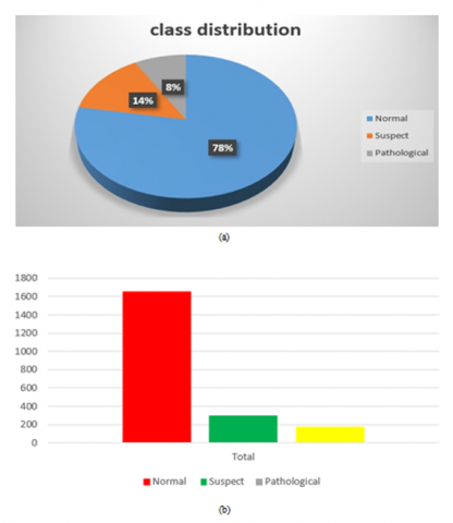
The University of California’s open-access Machine Learn- ing Repository provided the data set. It is a representation of 2,216 data points from third- trimester pregnant women. Below is a list of the 21 properties of these data points that have been used in this research to analyze FHR and uterine contraction on the CTG.
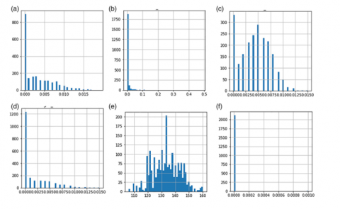
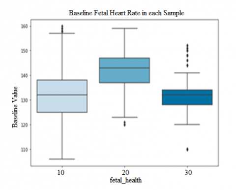
The entire data set is represented in different ways, the Figure 1 (a). The blue color in the figure represents the normal fetal count, green represents the pathological and the orange represents fetus in suspect. Likewise, the bar char is also shown in the Figure 1 (b) and Figure 2 represent the histogram of data. In the Figure 3 the box plot is shown, form the figure it can be infer that Base value, uterine contractions, fetal movement, abnormal short term variability, and histogram based parameters are the more impacting features considering all the parameters.
Figure 1. (a) Pie chart of the data set, (b) Bar chart of the data set
Figure 2. Histogram of individual features in the data set
Figure 3. Box plots of the data set
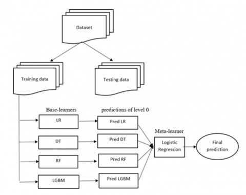
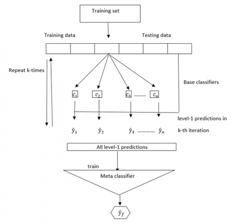
The main focus of this part is the process flow of fetal health classification using machine learning ensemble models. Figure 4 lays out the stages of the suggested procedure. The data is presented in a visually appealing format after being pre-processed.
Figure 4. Proposed model framework
Additionally, the data is divided into a test set and a train set. Both the base classifier's and the meta classifier's prediction effects impact the stack model ensemble learning technique's performance. The suggested ensemble model employs logistic regression as its meta classifier in addition to LR, DT, RFM, and LightGBM as its base classifiers. The following is a detailed explanation of the stack model.
3.1 Stack model
The terms stack model and stacked generalization refer to ensemble algorithms used in machine learning [25]. A meta-algorithm is employed to determine the optimal method for combining the results of multiple underlying machine learning algorithms [26]. Using a stack model's multiple efficient models, one can do classification or regression tasks and obtain results that surpass the performance of any single model used in the ensemble.
3.2 Basic architecture of stack model
In order to train the meta-model, the underlying models' non-sample data is extrapolated. A further way of looking at it is that the input/output pairings in the training set that the meta-model is adapted to are really the results that the base models were able to anticipate and produce using the data that wasn't utilized to train them. When it comes to regression, the basic models’ outputs can be real values, however when it comes to classification, they can be probability values, probability like values, or class labels.
3.3 Stack model ensemble method
Base learners: In this study, the union strategy creates a new set of features and then trains four basic learners, Logistic Regression, Decision Tree, Random Forest, and LightGBM—to use those features accurately.
Logistic Regression: Logistic regression is actually a progression of linear regression. Classical linear regression just performs regression and has the following fundamental structure:
$y=V^N x+a$ (1)
The problem of classification is solved by obtaining a pre- dicted value either 0 or 1 by linear regression [27]. However, linear regression produces the predicted value as a sequence of real values. The continuous function Sigmoid is then used to further alter it as a result:
$y=\frac{1}{1+e^{(-x)}}$ (2)
The sigmoid function can be used to translate the linear regression prediction result as a conditional probability to which the sample belongs to a specific class, and the classification result can then be produced using the predetermined classification threshold [28]. The belonging of the sample to positive and negative classes can be calculated by adding b to the weight vector A for the two-class problem:
$P(Y=1 \mid x)=\frac{\operatorname{Exp}(V \dot x)}{1+\operatorname{Exp}(V \dot x)}$ (3)
$P(Y=0 \mid x)=\frac{1}{1+\operatorname{Exp}(V \dot x)}$ (4)
In Eqs. (3) and (4) represent the logistic regression models. From the equation (3), if the linear function generates a value that increases to infinity, then the probability of the anticipated value belonging to a positive class and is nearer to 1, and otherwise it is nearer to 0. The box plots of the dataset are shown in Figure 3.
Decision Tree: In a decision tree, which is built on trees, each node along the way represents a data separation sequence that continues until the tree reaches a leaf node, where a Boolean result is obtained. It is structured using a node and a branch relationship, with nodes representing the goals of relational classification. Entropy and information gain are used in decision tree to make decision-making at various levels of nodes. When a node exclusively belongs to one class, entropy is 0. Entropy will be at its highest when the dataset is very disordered or when the classes are evenly split:
Entropy $=\sum_{i=1}^c-p_i * \log _2\left(p_i\right)$ (5)
Information Gain is used to quantify the dataset’s purity or homogeneity. Information gain is the distribution of data with regard to a response variable [22]. A variable is more informative and can be used as the root node if the information gain is large and split it if attribute has lower entropy. To create more manageable subsets of the dataset, the decision tree uses the information gain to acquire the attribute that does just that.
$\operatorname{Gain}(S, X)=\sum_{v \in V(X)} \frac{S_v}{S} \operatorname{Entropy}\left(S_v\right)$ (6)
where, V(X) is the range of features X and Sv is the subset of set S equal to the feature value of feature v.
Random Forest: The random forest employs the Gini index to determine if the nodes on the decision tree branch are associated or not. It is a multiple-decision set technique that may be used for regression and predictions. It classifies the data using a lot of decision trees:
Gini $=1-\sum_{i=1}^c\left(p_i\right)^2$ (7)
This formula was used to estimate the most likely branch on a node by computing the Gini of every branch according to the class and percentage. The overall number of classes in the data is represented by c, while the proportional prevalence of each class is represented by pi. The proposed model architecture is shown in Figure 4.
LightGBM: The LightGBM algorithm, which was derived from the GBDT method [29]. The method locates the leaf node from the already divided leaf nodes with the highest gain value; the depth of the tree is restricted to avoid over fitting and expedites the process of discovering the depth tree with optimal values. Additionally, if constant number of splits are maintained, then the error can be minimized and a maximum level of precision could be reached. Finding the optimum splitting node requires the greatest time and computing resources during the tree- building process. LightGBM uses a variety of strategies to achieve this, including the binding method, the histogram algorithm, gradient-based one- side sampling, and mutually exclusive features [30].
Meta-classifier: In our proposed work, logistic regression is presented as a solution to classification issues and is employed as a meta-classifier.
Ensemble of Classifiers: Figure 4 depicts the stack model ensemble learning prediction technique. Every single prediction model makes up the basic learner. First, multiple base learners are trained using the original dataset. Base learners are often trained using K-fold cross-validation during the training phase to lower the risk of model over fitting. The secondary learners are then taught to provide the final prediction outcomes after the base model’s prediction findings are combined into a new data set [31]. The Figure 5 shows the stages of the stack model algorithms and are explained in the below steps.
·First step is to separate the actual data set X into training data set Tr and the testing set Ts.
·On the base learner, do K-fold cross-validation by ran- domly by separating the actual training set Tr into K equivalents (Tr1, Tr2, ..., Trk), considering any one of them as K-fold test set, and rest of them as k-fold training set.
·The K-fold training set is used to train each base learner classifiers c1, c2,... , CK, predictions are formed using the K-fold test set, and the outcomes of each base learner’s classifiers are merged to form the secondary learner’s training set T¯r.
The stack model algorithm is shown in Figure 5.
Figure 5. Stack model algorithm
|
Algorithm |
|
INPUT: Consider training dataset $\operatorname{Tr}=\left\{x_i, y_i\right\}^m \quad\left(x_i \in X^n\right.$ $\left.y_i \in \mathrm{Y}\right)$ from $X$ OUTPUT: E, the ensemble classifier. Step1: Split the actual training set Tr into K equivalents (Tr1,Tr2,...,TrK) using k-fold validation. For all kin K do for all tints do step1.Learn the base classifier c1 based on Trk ENDFOR Define a new data set that contains $\left\{\bar{x}_i, y_i, \bar{x}_i=c_1\left(x_i\right), c_2\left(x_i\right), \ldots c T\left(x_i\right)\right\}$. step1.2 Next level classifier learning. For all $x_i \in \operatorname{Tr}_K$do Define a new data sets that contains $\bar{x}_{i, y_i}$, where $\bar{x}_i=c_1\left(x_i\right), c_2\left(x_i\right), \ldots c T\left(x_i\right)$. ENDFOR ENDFOR step2: Learning by second level classifier for all t in T do Learn the ct classifier ENDFOR Return $C(x)=\bar{c}\left(c_1\left(x_i\right), c_2\left(x_i\right), \ldots c T\left(x_i\right)\right)$ |
·Each base learner generates predictions on the initial test set Ts, and the secondary learners’ validation set T¯s which is created by averaging the prediction results.
·The training set T¯r and the validation set T¯s are obtained by the secondary learner, which then performs learning and training before producing the final prediction out- come.
The steps in the algorithm of the stack model are presented in algorithm 1. The K-fold cross-validation used in the stack model ensemble learning prediction approach lowers the likelihood that the model will become over fitted, and secondary training is carried out using the predictions of several base learners. This technique, which enhances the generalisation and accuracy of prediction outputs through machine learning, can get around the constraints of a single model and integrate variably with different models. The base model can select a strong learner, and the next stage model can select a simple learner when using stack model and improves the fusion effect and prevent over fitting.
Worldwide healthcare institutions have been grappling with the problem of infant mortality for decades. Despite our development of technologies that can measure numerous aspects of foetal health, reading and interpreting CTG data is not always achievable in places without a qualified obstetrician. Even in areas with access to medical experts, diagnosing a fetus one by one using CTG measurements [32] can be incredibly inefficient and time intensive. In contrast, fetal health may be classified by machine learning models in a fraction of the time it takes obstetricians to do so [33]. Machine learning models have the potential to provide practical answers to the foetal health problem due to their exceptionally precise predictions, but there have been significant obstacles to its widespread use, despite the technique's theoretical viability [34].
To begin, these models do not aid in pinpointing the source of the fetal pathology that has led to the diagnosis. If obstetricians are unable to determine the cause of the fetal distress, they will be unable to provide adequate care for their patients [35]. Another problem is that patients could not believe a machine's diagnosis if they can't comprehend the reasoning behind the model's conclusion.
Implementing an explainable model, which not only makes very accurate predictions but also explains to scientists how it made its conclusion, is the most effective strategy to address these issues [36]. When obstetricians have this information, they can better treat their patients by identifying the abnormal measurement and advising their patients on it. For example, if the model indicated a potentially dangerous foetal abnormality, it may also clarify how a low rate of uterine contractions influenced the prediction. Based on this information, the doctor can prescribe water and relaxation to help normalize levels, or in severe cases, medication like Oxytocin.
3.4 Stack model algorithm
In this proposed method we used, The University of Califor- nia’s open-access Machine Learning Repository provided the data set. The dataset can be splitted into 80% as training data 20% as testing data. In the suggested stack model ensemble learning algorithm, four ensemble machine learning algorithms like BOOSTING, ADABOOST, XGBoost, LightGBM are taken into consideration as base learners. Scikit Learn’s Grid output vector of the individual learners is stacked and given to the Logistic Regression as a meta learner; this module is designated as “Level 1” in the system architecture. The stack model is now prepared to make predictions using test data. Algorithm discusses the stack model Algorithm with cross validation used in this study.
4.1 Experimental setup
In order to find the accuracy of the stack model algorithm, The data set is obtained from the open-access Machine Learning Repository of the University of California. The data set contains the 21 features of fetal health classification with three classes: Normal, Suspect, and Pathology. The stack model algorithm was worked out with Python software on an i5 processor. The entire dataset can be divided into 80% used for training and 20% used for testing.
4.2 Quantitative analysis
Precision, recall, F1-score, and accuracy are the performance metrics used for quantitative analysis of the classification outcomes:
Precision $=\frac{T P}{T P+F P} * 100$ (8)
Recall $=\frac{T P}{T P+F N} * 100$ (9)
$F 1$ score $=2 * \frac{\text { Precision } * \text { Recall }}{\text { Precision }+ \text { Recall }}$ 10)
Accuracy $=\frac{T P+F N}{\mathrm{TP}+\mathrm{FN}+\mathrm{TN}+\mathrm{FN}}$ (11)
Kappa Score $=\frac{p_0-p_e}{1-p_e}$ (12)
where, TP: True positive; TN: True negative; FP: False positive; FN: False negative; pois the relative agreement among the classes; pethe hypothetical probability of change of class.
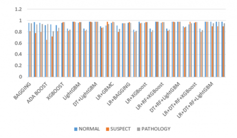
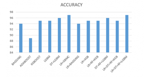
The F1-score, precision, recall and accuracy measures are given in Table 1. These performance measures are calculated for fetal health classification, namely, normal, suspect, and pathology, as typical in the open-access Machine Learning Repository of the University of California. The results proved that the stack model algorithm had extracted the classes of fetal accurately than other considered models in Table 1. The graphical representation of the performance measures is shown in Figure 6 and Figure 7. From the visual analysis it can see that the stack model is performing well.
Figure 6. Comparison of performance measures
Out of a total of 324 normal classes, the Bagging model correctly identified 315 as normal, mislabeled 9 as suspect, and 0 as pathology. Similarly, out of 60 suspect classes, 46 were incorrectly classified as suspect, 13 were correctly classified as normal, and 1 as pathology. Out of a total of 42 pathologies, 38 were incorrectly classed as normal, while 1 was considered suspicious. You may find the corresponding confusion matrix in Table 2. Based on these classification results, the Bagging model performed extremely well, with a precision value of 0.96%, a suspect value of 0.81%, and a pathology value of 0.95%. The recall value was 0.97%, the suspect value was 0.78%, and the pathology value was 0.93%. The F1-score value was 0.96%, the suspect value was 0.80%, and the pathology value was 0.94%. The model's overall accuracy was 94%. Out of a total of 324 normal classes, the AdaBoost model correctly identified 300 as normal, 22 as suspect, and 2 as pathology. Of the 60 suspect classes, 43 were incorrectly classified as suspect, 17 as normal, and 0 as pathology. Out of a total of 42 pathologies, 34 were incorrectly labeled as normal, and 0 were deemed suspicious. You may find the corresponding confusion matrix in Table 2. Based on these classification results, the AdaBoost model performed to specification with a normal precision of 0.92%, a suspect precision of 0.66%, and a pathology precision of 0.94%; a recall of 0.93%, a suspect precision of 0.72%, and a pathology F1-score of 0.87%; and an overall accuracy of 89%.
Figure 7. Comparison of accuracy
Table 1. Performance measure of the models
|
Model |
Metric |
Normal |
Suspect |
Pathology |
|
BAGGING |
Precision |
0.96 |
0.81 |
0.95 |
|
Recall |
0.97 |
0.78 |
0.93 |
|
|
F1-Score |
0.96 |
0.80 |
0.94 |
|
|
Support |
324 |
60 |
42 |
|
|
Accuracy |
94% |
|||
|
ADA BOOST |
Precision |
0.92 |
0.66 |
0.94 |
|
Recall |
0.93 |
0.72 |
0.81 |
|
|
F1-Score |
0.92 |
0.81 |
0.87 |
|
|
Support |
324 |
60 |
42 |
|
|
Accuracy |
89% |
|||
|
XGBoost |
Precision |
0.96 |
0.97 |
0.97 |
|
Recall |
0.86 |
0.82 |
0.84 |
|
|
F1-Score |
0.98 |
0.98 |
0.97 |
|
|
Support |
324 |
60 |
42 |
|
|
Accuracy |
95% |
|||
|
LightGBM |
Precision |
0.96 |
0.97 |
0.97 |
|
Recall |
0.86 |
0.82 |
0.84 |
|
|
F1-Score |
0.98 |
0.98 |
0.97 |
|
|
Support |
324 |
60 |
42 |
|
|
Accuracy |
95% |
|||
|
DT+LightGBM |
Precision |
0.98 |
0.98 |
0.98 |
|
Recall |
0.90 |
0.87 |
0.88 |
|
|
F1-Score |
0.91 |
0.98 |
0.94 |
|
|
Support |
324 |
60 |
42 |
|
|
Accuracy |
96% |
|||
|
LR+GBMC |
Precision |
0.96 |
0.98 |
0.97 |
|
Recall |
0.91 |
0.80 |
0.85 |
|
|
F1-Score |
0.95 |
0.95 |
0.95 |
|
|
Support |
324 |
60 |
42 |
|
|
Accuracy |
96% |
|||
|
LR+BAGGING |
Precision |
0.96 |
0.97 |
0.96 |
|
Recall |
0.84 |
0.80 |
0.82 |
|
|
F1-Score |
0.98 |
0.95 |
0.96 |
|
|
Support |
324 |
60 |
42 |
|
|
Accuracy |
94% |
|||
|
LR+XGBoost |
Precision |
0.96 |
0.97 |
0.97 |
|
Recall |
0.86 |
0.80 |
0.83 |
|
|
F1-Score |
0.98 |
0.98 |
0.98 |
|
|
Support |
324 |
60 |
42 |
|
|
Accuracy |
95% |
|||
|
LR+RF+XGBoost |
Precision |
0.96 |
0.97 |
0.97 |
|
Recall |
0.86 |
0.82 |
0.84 |
|
|
F1-Score |
0.98 |
0.98 |
0.97 |
|
|
Support |
324 |
60 |
42 |
|
|
Accuracy |
95% |
|||
|
DT+RF+LightGBM |
Precision |
0.98 |
0.98 |
0.98 |
|
Recall |
0.90 |
0.88 |
0.89 |
|
|
F1-Score |
0.93 |
0.98 |
0.95 |
|
|
Support |
324 |
60 |
42 |
|
|
Accuracy |
96% |
|||
|
LR+DT+RF+XGBoost |
Precision |
0.96 |
0.97 |
0.97 |
|
Recall |
0.86 |
0.80 |
0.83 |
|
|
F1-Score |
0.98 |
0.98 |
0.98 |
|
|
Support |
324 |
60 |
42 |
|
|
Accuracy |
95% |
|||
|
LR+DT+RF+LightGBM |
Precision |
0.97 |
0.98 |
0.98 |
|
Recall |
0.89 |
0.85 |
0.87 |
|
|
F1-Score |
0.93 |
0.95 |
0.94 |
|
|
Support |
324 |
60 |
42 |
|
|
Accuracy |
96.71% |
|||
Table 2. Confusion matrix of the models
|
Model |
Class |
Normal |
Suspect |
Pathology |
Total |
|
BAGGING |
Normal |
315 |
9 |
0 |
324 |
|
Suspect |
13 |
46 |
1 |
60 |
|
|
Pathology |
3 |
1 |
38 |
42 |
|
|
ADA BOOST |
Normal |
300 |
22 |
2 |
324 |
|
Suspect |
17 |
43 |
0 |
60 |
|
|
Pathology |
8 |
0 |
34 |
42 |
|
|
XGBoost |
Normal |
315 |
8 |
1 |
324 |
|
Suspect |
12 |
48 |
0 |
60 |
|
|
Pathology |
1 |
0 |
41 |
42 |
|
|
LightGBM |
Normal |
315 |
8 |
1 |
324 |
|
Suspect |
12 |
48 |
0 |
60 |
|
|
Pathology |
1 |
0 |
41 |
42 |
|
|
DT+LightGBM |
Normal |
317 |
6 |
1 |
324 |
|
Suspect |
5 |
52 |
3 |
60 |
|
|
Pathology |
1 |
0 |
41 |
42 |
|
|
LR+GBMC |
Normal |
319 |
4 |
1 |
324 |
|
Suspect |
12 |
48 |
0 |
60 |
|
|
Pathology |
2 |
0 |
40 |
42 |
|
|
LR+BAGGING |
Normal |
314 |
9 |
1 |
324 |
|
Suspect |
12 |
48 |
0 |
60 |
|
|
Pathology |
2 |
0 |
40 |
42 |
|
|
LR+XGBoost |
Normal |
315 |
8 |
1 |
324 |
|
Suspect |
12 |
48 |
0 |
60 |
|
|
Pathology |
1 |
0 |
41 |
42 |
|
|
LR+RF+XGBoost |
Normal |
315 |
8 |
1 |
324 |
|
Suspect |
11 |
49 |
0 |
60 |
|
|
Pathology |
1 |
0 |
41 |
42 |
|
|
DT+RF+LightGBM |
Normal |
317 |
6 |
1 |
324 |
|
Suspect |
5 |
52 |
3 |
60 |
|
|
Pathology |
1 |
0 |
41 |
42 |
|
|
DT+LR+XGBoost |
Normal |
315 |
8 |
1 |
324 |
|
Suspect |
11 |
49 |
0 |
60 |
|
|
Pathology |
1 |
0 |
41 |
42 |
|
|
LR+DT+RF+XGBoost |
Normal |
315 |
8 |
1 |
324 |
|
Suspect |
12 |
48 |
0 |
60 |
|
|
Pathology |
1 |
0 |
41 |
42 |
|
|
LR+DT+RF+LightGBM |
Normal |
317 |
6 |
1 |
324 |
|
Suspect |
5 |
54 |
1 |
60 |
|
|
Pathology |
1 |
0 |
41 |
42 |
Out of a total of 324 normal classes, the XGBoost model correctly identified 315 as normal, mislabeled 8 as suspect, and categorized 1 as pathology. Similarly, out of 60 suspect classes, 48 were incorrectly classified as suspect, 12 as normal, and 0 as pathology. We incorrectly identified one case as normal and zero as questionable out of a total of forty-two pathologies. You may find the corresponding confusion matrix in Table 2. The XGBoost model performed admirably in this classification task, with normal, suspect, and pathology precision values of 0.97%, 0.86%, and 0.83%, respectively. The model also achieved an F1-score of 0.98%, suspect 0.98%, and pathology 0.98%, and an overall accuracy of 95%.
The LightGBM model correctly identified 315 out of 324 normal cases, mislabeled 8 as suspect cases, and categorized 1 as pathology. Of the 60 cases in the suspicious class, 48 were erroneously classified as suspect cases, 12 as normal, and 0 as pathology. We incorrectly identified one case as normal and zero as questionable out of a total of forty-two pathologies. You may find the corresponding confusion matrix in Table 2. Based on these classification results, the LightGBM model performed admirably, with standard accuracy of 0.96%, suspect accuracy of 0.97%, and pathology accuracy of 0.97%; recall values of 0.96%, suspect accuracy of 0.80%, and pathology accuracy of 0.83%; F1-score values of 0.98%, suspect accuracy of 0.98%, and pathology accuracy of 0.98%; and overall accuracy of 95%.
We incorrectly identified one case as normal and zero as questionable out of a total of forty-two pathologies. You may find the corresponding confusion matrix in Table 2. Here are the classification results: the DT+LightGBM model achieved a performance of 0.98% for normal, 0.90% for suspect, and 0.91% for pathology; 0.98% for recall, 0.87% for suspect, and 0.98% for pathology; 0.98% for F1-score, 0.88% for suspect, and 0.94% for pathology; and a total accuracy of 96%.
Out of a total of 324 normal classes, the LR+GBMC model correctly identified 319 as normal, mislabeled 4 as suspicious, and labelled 1 as pathology. Similarly, out of 60 questionable classes, 48 were incorrectly classified as suspect, 11 as normal, and 1 as pathology. We incorrectly identified one case as normal and zero as questionable out of a total of forty-two pathologies. You may find the corresponding confusion matrix in Table 2. The LR+GBMC model achieved a 96% overall accuracy with these classification results: normal precision = 0.96%, suspect 0.91%, and pathology 0.95%; recall = 0.98%, suspect = 0.80%, and pathology = 0.95%; F1-score = 0.97%, suspect = 0.95%, and pathology = 0.95%.
Out of a total of 324 normal classes, the LR+BAGGING model correctly identified 314 as normal, mislabeled 9 as suspicious, and categorized 1 as pathology. Similarly, out of 60 suspect classes, 48 were incorrectly classified as suspect, 12 as normal, and 0 as pathology. Out of a total of 42 pathologies, 40 were incorrectly labeled as normal and 1 as questionable. You may find the corresponding confusion matrix in Table 2. The LR+BAGGING model achieved a 94% overall accuracy rate based on these classification results: normal 0.96% precision, suspect 0.84%, and pathology 0.98% recall; suspect 0.80% and pathology 0.95%, respectively, and F1-score values of 0.96%, 0.82%, and 0.96%, respectively, for normal and suspect categories.
Out of a total of 324 normal classes, the LR+XGBoost model correctly identified 315 as normal, mislabeled 8 as suspect, and categorized 1 as pathology. Similarly, out of 60 suspect classes, 48 were incorrectly classified as suspect, 12 as normal, and 0 as pathology. We incorrectly identified one case as normal and zero as questionable out of a total of forty-two pathologies. You may find the corresponding confusion matrix in Table 2. The LR+XGBoost model achieved a 95% overall accuracy with these classification results: normal precision = 0.96%, suspect 0.86%, and pathology 0.98%; recall = 0.97%, suspect 0.80%, and pathology 0.98%; F1-score = 0.97%, suspect 0.83%, and pathology 0.98%.
Out of 324 normal cases, 8 were incorrectly categorized as suspect and 1 as pathology by the LR+RF+XGBoost model. Of 60 suspect cases, 49 were incorrectly classified as suspect, 11 were correctly classified as normal, and 0 were classified as pathology. We incorrectly identified one case as normal and zero as questionable out of a total of forty-two pathologies. You may find the corresponding confusion matrix in Table 2. The LR+RF+XGBoost model was able to achieve a 95% overall accuracy rate based on these classification results: normal performance: 0.96%, suspect performance: 0.86%, and pathology performance: 0.98%. Normal recall: 0.97%, suspect performance: 0.82%, and pathology performance: 0.98%. F1-score: 0.97%, suspect performance: 0.84%, and pathology performance: 0.98%.
Out of a total of 324 normal classes, the DT+RF+LightGBM model correctly identified 317 as normal, incorrectly classified 6 as suspect, and further mislabeled 1 as pathology. Of the 60 suspect classes, 52 were classified as suspect and incorrectly, 5 as normal, and 3 as pathology. We incorrectly identified one case as normal and zero as questionable out of a total of forty-two pathologies. You may find the corresponding confusion matrix in Table 2. Based on these classification results, the DF+RF+LightGBM model achieved a 96% overall accuracy, with a recall of 0.98%, a suspect of 0.88%, and a pathology of 0.98%; an F1-score of 0.98%, a suspect of 0.89%, and a pathology of 0.95%; and overall precision of 0.98%, 0.90%, and 0.93%, respectively.
Out of a total of 324 normal classes, the LR+DT+RF+XGBoost model correctly identified 315 as normal, mislabeled 8 as suspect, and categorized 1 as pathology. Similarly, out of 60 suspect classes, 48 were incorrectly classified as suspect, 12 as normal, and 0 as pathology. We incorrectly identified one case as normal and zero as questionable out of a total of forty-two pathologies. You may find the corresponding confusion matrix in Table 2. Here are the classification results for the LR+DT+RF+XGBoost model: normal performance: 0.96%, suspect 0.86%, and pathology 0.98%; recall: 0.97%, suspect 0.80%, and pathology 0.98%; F1-score: 0.97%, suspect 0.83%, and pathology 0.98%; and overall accuracy: 95%.
Out of 324 normal cases, 5 were incorrectly classified as suspects and 1 as pathology by the LR+DT+RF+LightGBM model. Of 60 suspect cases, 53 were incorrectly classified as suspects, 6 were correctly classified as normal, and 1 was classified as pathology. We incorrectly identified one case as normal and zero as questionable out of a total of forty-two pathologies. You may find the corresponding confusion matrix in Table 2. Based on these classification results, the LR+DT+RF+LightGBM model performed admirably. Its precision value was 0.97% for normal, 0.98% for suspect, and 0.98% for pathology. The recall value was 0.89% for normal, 0.85% for suspect, and 0.87% for pathology. The F1-score value was 0.93% for normal, 0.95% for suspect, and 0.94% for pathology. The overall accuracy was 96.71%. With a kappa score of 0.9167, the evaluated stack ensemble model outperforms the state-of-the-art models. An argument in favor of the stack model might be made that the Staking ensemble learning method has significantly enhanced the evaluation of the base learning model. Comparing the suggested model's performance to that of prior research models is shown in Table 3.
Table 3. Comparison between the proposed model and previous researchers’ models
|
Methodology |
Dataset and Predict Classes |
Accuracy (%) |
F1-Score |
Kappa Score |
|
Deep Forest [27], 2021 |
21,3 |
95.07 |
0.9201 |
- |
|
Random Forest [28], 2021 |
10,3 |
92.01 |
0.8262 |
0.8262 |
|
Support Vector Machine [29], 2019 |
21,3 |
92.39 |
0.8424 |
- |
|
Random Forest [30], 2019 |
21,3 |
94.8 |
0.948 |
- |
|
Na¨ıve Bayes [31], 2019 |
16,3 |
85.88 |
0.895 |
- |
|
Random Forest [32], 2019 |
21,3 |
95.11 |
- |
- |
|
CART with Gini Index [15], 2018 |
21,3 |
90.12 |
0.9 |
- |
|
Random Forest [33], 2018 |
21,3 |
93.4 |
- |
0.817 |
|
META-DES, ensemble classifier [34], 2015 |
21,3 |
84.62 |
- |
- |
|
Bagging based Random Forest [35], 2015 |
21,3 |
94.73 |
0.9047 |
- |
|
stacking Ensemble Learning [4], 2021 |
10,3 |
96.05 |
- |
0.8875 |
|
Stacked model [36], 2021 |
21,3 |
96.08 |
0.9336 |
- |
|
Stack model |
21,3 |
96.71 |
0.94 |
0.9167 |
Prevention and reduction of perinatal mortality can be achieved through accurate fetal health prediction or identification. Reports from CTG tests can be sorted into one of three categories based on the FHR, FHR fluctuation, decelerations, and accelerations: suspicious, normal, or pathological. This research presents a stack model based method for fetal health classification. We introduced the stack model, an ensemble approach, and showed how it was used to classify foetal health using the FHR dataset. The benefit of a stack model is that it can outperform any individual model in an ensemble by utilizing multiple effective models to complete classification or regression tasks and generate predictions. When it comes to non-invasive and cost-effective methods of continuously monitoring the health of the fetus, CTG is currently your sole option. Despite the rise of automation, CTG analysis remains a challenging signal processing operation. The intricate and dynamic patterns of the developing foetal heart are challenging to understand. In instance, there is a general trend toward exceedingly imprecise human and machine evaluations of suspicious cases. In addition, the initial and second stages of labor have significantly different dynamics of the FHR. The performance of the proposed algorithm stack model is compared and experimented with various Machine learning Techniques namely Boosting, Ada boosting and XGBoost and LightGBM, DT+LightGBM, LR+LightGBM, LR+BAGGING, LR+XGBoost, LR+RF+XGBoost, DT+RF+LightGBM, LR+DT+RF+XGBoost, LR+DT+RF+LightGBM and the classification accuracy of the respective algorithms are 94%, 89%, 95%, 95%, 96%, 96%, 94%, 95%, 95%, 96%, 95%. Compared to its predecessors, the stack model is superior, having attained a performance level of 96.71%. The suggested approach outperforms the previously considered state-of-the-art machine learning algorithms when it comes to classifying fetal health using FHR data. With the given training data and in the ensemble models under consideration, the suggested model is run. Additional samples necessitate enhancements. Becoming hybrid and combining the strengths of many models and optimization methodologies might further improve the model. To determine the optimal fitness value for precise health categorization, hybrid optimization techniques like Particle Swarm Optimization and Artificial Bee Colony Optimization can be utilized. For improved precision, deep learning models such as ResNet50 can be used.
[1] Spilka, J., Frecon, J., Leonarduzzi, R., Pustelnik, N., Abry, P., Doret, M. (2016). Sparse support vector machine for intrapartum fetal heart rate classification. IEEE Journal of Biomedical and Health Informatics, 21(3): 664-671. https://doi.org/10.1109/JBHI.2016.2546312
[2] Arif, M.Z., Ahmed, R., Sadia, U.H., Tultul, M.S.I., Chakma, R. (2020). Decision tree method using for fetal state classification from cardiotography data. Journal of Advanced Engineering and Computation, 4(1): 64-73. http://doi.org/10.25073/jaec.202041.273
[3] Subasi, A., Kadasa, B., Kremic, E. (2020). Classification of the cardiotocogram data for anticipation of fetal risks using bagging ensemble classifier. Procedia Computer Science, 168: 34-39. https://doi.org/10.1016/j.procs.2020.02.248
[4] Bhowmik, P., Bhowmik, P.C., Ali, U.M.E., Sohrawordi, M. (2021). Cardiotocography data analysis to predict fetal health risks with tree-based ensemble learning. International Journal of Information Technology and Computer Science, 5: 30-40. https://doi.org/10.5815/ijitcs.2021.05.03
[5] Chen, J.Y., Liu, X.C., Wei, H., Chen, Q.Q., Hong, J.M., Li, Q.N., Hao, Z.F. (2019). Imbalanced cardiotocography multi-classification for antenatal fetal monitoring using weighted random forest. In Smart Health: International Conference, ICSH 2019, Shenzhen, China, July 1-2, 2019, Proceedings 7, pp. 75-85. https://doi.org/10.1007/978-3-030-34482-5_7
[6] Iraji, M.S. (2019). Prediction of fetal state from the cardiotocogram recordings using neural network models. Artificial Intelligence in Medicine, 96: 33-44. https://doi.org/10.1016/j.artmed.2019.03.005
[7] Ponsiglione, A.M., Cosentino, C., Cesarelli, G., Amato, F., Romano, M. (2021). A comprehensive review of techniques for processing and analyzing fetal heart rate signals. Sensors, 21(18): 6136. https://doi.org/10.3390/s21186136
[8] Liu, L., Jiao, Y., Li, X., Ouyang, Y., Shi, D. (2020). Machine learning algorithms to predict early pregnancy loss after in vitro fertilization-embryo transfer with fetal heart rate as a strong predictor. Computer Methods and Programs in Biomedicine, 196: 105624. https://doi.org/10.1016/j.cmpb.2020.105624
[9] Ogunyemi, D., Jovanovski, A., Friedman, P., Sweatman, B., Madan, I. (2019). Temporal and quantitative associations of electronic fetal heart rate monitoring patterns and neonatal outcomes. The Journal of Maternal-Fetal & Neonatal Medicine, 32(18): 3115-3124. https://doi.org/10.1080/14767058.2018.1456523
[10] Kong, Y., Xu, B., Zhao, B., Qi, J. (2021). Deep gaussian mixture model on multiple interpretable features of fetal heart rate for pregnancy wellness. In Pacific-Asia Conference on Knowledge Discovery and Data Mining, pp. 238-250. https://doi.org/10.1007/978-3-030-75762-5_20
[11] Avuçlu, E., Elen, A. (2020). Classification of cardiotocography records with Naïve Bayes. International Scientific and Vocational Studies Journal, 3(2): 105-110.
[12] Haque, E., Gupta, T., Singh, V., Nene, K., Masurkar, A. (2022). Detection and classification of fetal heart rate (FHR). In International Conference on Artificial Intelligence and Sustainable Engineering: Select Proceedings of AISE 2020, pp. 437-447. https://doi.org/10.1007/978-981-16-8542-2_35
[13] Cömert, Z., Boopathi, A.M., Velappan, S., Yang, Z., Kocamaz, A.F. (2018). The influences of different window functions and lengths on image-based time-frequency features of fetal heart rate signals. In 2018 26th Signal Processing and Communications Applications Conference (SIU), pp. 1-4. https://doi.org/10.1109/SIU.2018.8404247
[14] Chauhan, V.K., Dahiya, K., Sharma, A. (2019). Problem formulations and solvers in linear SVM: A review. Artificial Intelligence Review, 52(2): 803-855. https://doi.org/10.1007/s10462-018-9614-6
[15] Ramla, M., Sangeetha, S., Nickolas, S. (2018). Fetal health state monitoring using decision tree classifier from cardiotocography measurements. In 2018 Second International Conference on Intelligent Computing and Control Systems (ICICCS), pp. 1799-1803. https://doi.org/10.1109/ICCONS.2018.8663047
[16] Kumar, G.R., Sheshanna, K.V., Basha, S.R., Reddy, P.K.K. (2021). An improved decision tree classification approach for expectation of cardiotocogram. In Proceedings of International Conference on Computational Intelligence, Data Science and Cloud Computing: IEM-ICDC 2020, pp. 327-333. https://doi.org/10.1007/978-981-33-4968-1_26
[17] Kuo, P.L., Yen, L.B., Du, Y.C., Chen, P.F., Tsai, P.Y. (2021). Combination of XGBoost analysis and rule-based method for intrapartum cardiotocograph classification. Journal of Medical and Biological Engineering, 41(4): 534-542. https://doi.org/10.1007/s40846-021-00642-y
[18] Lu, Y., Fu, X., Chen, F., Wong, K.K. (2020). Prediction of fetal weight at varying gestational age in the absence of ultrasound examination using ensemble learning. Artificial Intelligence in Medicine, 102: 101748. https://doi.org/10.1016/j.artmed.2019.101748
[19] Ma, Y., Xiao, Y., Wei, G., Sun, J. (2018). Foetal ECG extraction using non-linear adaptive noise canceller with multiple primary channels. IET Signal Processing, 12(2): 219-227. https://doi.org/10.1049/iet-spr.2016.0605
[20] Otchere, D.A., Ganat, T.O.A., Gholami, R., Lawal, M. (2021). A novel custom ensemble learning model for an improved reservoir permeability and water saturation prediction. Journal of Natural Gas Science and Engineering, 91: 103962. https://doi.org/10.1016/j.jngse.2021.103962
[21] Schober, P., Vetter, T.R. (2021). Logistic regression in medical research. Anesthesia and Analgesia, 132(2): 365. https://doi.org/10.1213/ANE.0000000000005247
[22] Charbuty, B., Abdulazeez, A. (2021). Classification based on decision tree algorithm for machine learning. Journal of Applied Science and Technology Trends, 2(01): 20-28. https://doi.org/10.38094/jastt20165
[23] Hafiz, P., Nematollahi, M., Boostani, R., Jahromi, B.N. (2017). Predicting implantation outcome of in vitro fertilization and intracytoplasmic sperm injection using data mining techniques. International Journal of Fertility & Sterility, 11(3): 184-190. https://doi.org/10.22074/ijfs.2017.4882
[24] Ke, G., Meng, Q., Finley, T., Wang, T., Chen, W., Ma, W., Ye, Q.W., Liu, T.Y. (2017). LightGBM: A highly efficient gradient boosting decision tree. Advances in Neural Information Processing Systems, 30.
[25] Zhu, H., Li, Y., Li, R., Li, J., You, Z., Song, H. (2020). SEDMDroid: An enhanced stacking ensemble framework for Android malware detection. IEEE Transactions on Network Science and Engineering, 8(2): 984-994. https://doi.org/10.1109/TNSE.2020.2996379
[26] Pedregosa, F., Varoquaux, G., Gramfort, A., Michel, V., Thirion, B., Grisel, O., et al. (2011). Scikit-learn: Machine learning in Python. The Journal of Machine Learning Research, 12: 2825-2830.
[27] Chen, Y., Guo, A., Chen, Q., Quan, B., Liu, G., Li, L., Hong, J.M., Hao, Z. (2021). Intelligent classification of antepartum cardiotocography model based on deep forest. Biomedical Signal Processing and Control, 67: 102555. https://doi.org/10.1016/j.bspc.2021.102555
[28] Prasetyo, S.E., Prastyo, P.H., Arti, S. (2021). A cardiotocographic classification using feature selection: A comparative study. JITCE (Journal of Information Technology and Computer Engineering), 5(01): 25-32. https://doi.org/10.25077/jitce.5.01.25-32.2021
[29] Agrawal, K., Mohan, H. (2019). Cardiotocography analysis for fetal state classification using machine learning algorithms. In 2019 International Conference on Computer Communication and Informatics (ICCCI), pp. 1-6. https://doi.org/10.1109/ICCCI.2019.8822218
[30] Imran Molla, M.M., Jui, J.J., Bari, B.S., Rashid, M., Hasan, M.J. (2021). Cardiotocogram data classification using random forest based machine learning algorithm. In Proceedings of the 11th National Technical Seminar on Unmanned System Technology 2019: NUSYS'19, pp. 357-369. https://doi.org/10.1007/978-981-15-5281-6_25
[31] Afridi, R., Iqbal, Z., Khan, M., Ahmad, A., Naseem, R. (2019). Fetal heart rate classification and comparative analysis using cardiotocography data and KNOWN classifiers. International Journal of Grid and Distributed Computing (IJGDC), 12: 31-42.
[32] Islam, S., Yulita, I. (2020). Predicting fetal condition from cardiotocography results using the random forest method. In Proceedings of the 7th Mathematics, Science, and Computer Science Education International Seminar, MSCEIS 2019, 12 October 2019, Bandung, West Java, Indonesia. http://dx.doi.org/10.4108/eai.12-10-2019.2296540
[33] Sontakke, S.A., Lohokare, J., Dani, R., Shivagaje, P. (2019). Classification of cardiotocography signals using machine learning. In Intelligent Systems and Applications: Proceedings of the 2018 Intelligent Systems Conference (IntelliSys), pp. 439-450. https://doi.org/10.1007/978-3-030-01057-7_35
[34] Cruz, R.M., Sabourin, R., Cavalcanti, G.D., Ren, T.I. (2015). META-DES: A dynamic ensemble selection framework using meta-learning. Pattern Recognition, 48(5): 1925-1935. https://doi.org/10.1016/j.patcog.2014.12.003
[35] Shah, S.A.A., Aziz, W., Arif, M., Nadeem, M.S.A. (2015). Decision trees based classification of cardiotocograms using bagging approach. In 2015 13th international conference on frontiers of information technology (FIT), pp. 12-17. https://doi.org/10.1109/FIT.2015.14
[36] Feng, J., Liang, J., Qiang, Z., Li, X., Chen, Q., Liu, G., Hong, J.M., Hao, Z.F., Wei, H. (2021). Effective techniques for intelligent cardiotocography interpretation using XGB-RF feature selection and stacking fusion. In 2021 IEEE International Conference on Bioinformatics and Biomedicine (BIBM), pp. 2667-2673. https://doi.org/10.1109/BIBM52615.2021.9669694