Hassan Muwafaq Gheni*![]() | Laith A. Abdul-Rahaim
| Laith A. Abdul-Rahaim![]()
© 2024 The authors. This article is published by IIETA and is licensed under the CC BY 4.0 license (http://creativecommons.org/licenses/by/4.0/).
OPEN ACCESS
Intelligent Transportation Systems (ITS) have extensively utilized driver behavior monitoring systems to mitigate the risk of traffic accidents caused by factors such as aggression and distraction. However, existing methods often rely on computer vision techniques, raising concerns about privacy violations and vulnerability to spoofing attacks. These attacks can potentially result in inaccurate analysis of driver behavior and compromise the effectiveness of the system. To mitigate this issue, the proposed system relies on in-vehicle sensors and the driving signal obtained from the CAN-BUS, which provide direct and reliable measurements of driver behavior. By analyzing real-time data collected from multiple drivers, the hybrid deep learning model is trained to recognize patterns and characteristics indicative of safe and unsafe driving behavior. The driving signal obtained from the Controller Area Network bus (CAN-BUS), including acceleration, RPM, speed, accelerator pedal value, and throttle position signal, etc., is utilized to recognize safe and unsafe driver behavior. The utilization of a hybrid deep learning model, which combines Convolutional Neural Network (CNN) and Long Short-Term Memory (LSTM), is a deliberate choice in order to harness the respective advantages of both methods. This decision is driven by the aim to overcome the challenges encountered by previous approaches by capitalizing on the strengths of CNN and LSTM. The model is trained and tested on a real-time dataset collected from multiple drivers. Experimental results demonstrate the effectiveness of the proposed method in accurately detecting driver behavior, addressing the public health concern of traffic accidents.
road safety, driver behaviour, deep learning, hybrid model, CAN-BUS
To ensure safe and responsible driving, drivers must remain fully attentive to their performance and diligently concentrate on the road ahead of them [1]. Unfortunately, the driver's consideration can be easily diverted by various activities, events, and surroundings, leading to distractions that can compromise safe driving practices [2]. Driver distraction may occur in a variety of ways, such as visual (when a driver's eyes are taken off the road), manual (when a driver's hands are taken off the wheel), and cognitive (when a driver loses concentration on the road) [3]. These types of distractions can significantly increase the risk of a car crash or other types of accidents.
The increasing usage of vehicles in modern times has resulted in undesirable consequences, such as traffic congestion, accidents, injuries, fatalities, and financial losses. A survey conducted by the National Highway Traffic Safety Administration (NHTSA) and Virginia Tech Transportation Institute (VTTI) revealed that a minimum of 80% of accidents and 65% of near-accidents that take place every day on roads and highways are associated with distractions or poor decision-making while driver driving on roads and highways [4, 5]. Additionally, secondary tasks such as visual, auditory, and haptic-related tasks, like using vehicle displays, listening to the radio, or using a smartphone, can still affect driving safety [6].
The concept of driver behaviour is intricate and pertains to the Driver's ability to manage and control the vehicle in a specific environment and context for each driving scenario [7]. The Driver plays a crucial role in ensuring driving safety as they manage and manoeuvre the vehicle through a set of actions.
Research and technology advancements have led to significant developments in driver behavior detection. Various approaches are being explored, including computer vision-based methods, sensor-based techniques, biometric data analysis, and machine learning algorithms [8-15]. Computer vision techniques employ cameras and video data to track driver behavior, facial expressions, and eye movements, enabling detection of distractions and fatigue. However, concerns regarding privacy violations and occasional failures in specific situations have been raised despite notable progress in computer vision and camera-based human identification.
However, combining these technologies can help us get closer to our objective of creating a reliable end to end system for tracking the risk of driver distraction in commonplace circumstances [16]. An offering method for tracking drivers' actions as well as carrying out modern technology and advances in artificial intelligence (AI) gives us various capabilities that can significantly expand our potential in this area [17]. Improved CAN-BUS and electronics have also been developed for analysis, real-time monitoring, reporting, and command over potentially distracting automated decision-making by applying deep learning to big datasets generated via CAN-BUS sensor.
To achieve the highest accuracy with the smallest time window size and the least amount of data, we propose an in-vehicle sensor based system for the detection of aggressive driving in real-time behaviours using Convolutional Neural Networks (CNN) combined with Recurrent Neural Networks (RNN/LSTM). The following contributions assist the paper in achieving its main goal.
An efficient deep-learning model is proposed to detect aggressive Driver behaviour utilizing in-vehicle data from CAN-BUS sensor. The architecture we have proposed achieves better performance than existing state-of-the-art methods. It demonstrates improved accuracy, effective memory use, and reduced computational complexity.
Our proposed framework for driver behaviour can achieve classification with a shorter time-series window as compared to prior research.
Our study specifically examines the impact of anomaly data presence and window size, which refers to the number of time steps and the level of overlap achieved through sliding windows, on the accuracy of the results.
Classification of driving behaviour has received a lot of research over the past few years. To develop a self-driving system, preliminary research has been done to develop dynamic models of the interaction between humans and vehicles [18].
The most dependable way to collect data from naturalistic experiments is to use in-vehicle sensors, which is recommended [19-21]. These include requiring drivers to repeatedly perform synthetic tasks aggressively and safely when performing manoeuvres in a controlled setting, such as braking, accelerating, turning, etc. One method that is not feasible for obtaining ground truth data on unsafe driving is to request individuals to engage in risky driving behaviour on public roads on purpose was done to more accurately identify driving manoeuvres like starting, stopping, passing, etc. [22-24]. Driver behavior analysis using CAN-BUS data has garnered significant attention, utilizing various techniques ranging from traditional methods to machine learning and deep learning approaches.
Different ML tools have been successfully applied in this field using supervised and unsupervised learning methods. One of the primary challenges facing supervised learning models in classifying driving styles is the lack of external knowledge or "ground truth" regarding what constitutes safe versus unsafe driving. However, unsupervised models rarely succeed in producing classifications that can be directly connected to driving safety. Several methods for labelling driving behaviour have been suggested in research utilizing supervised learning methods [25].
2.1 Traditional machine learning techniques
In recent years, machine learning techniques have gained prominence, enabling automated feature extraction and modeling of driver behavior. Algorithms such as decision trees, random forests, and support vector machines have been used to classify driver actions based on CAN-BUS and IMU data.
Chen et al. [26] used an inertial measuring unit (IMU) sensor to examine drivers' behavior when making left- and right-hand turns. To identify the Driver when turning, the scholar observed the characteristics provided. The vehicle's acceleration at the end of the arch and the deviation of the given acceleration along the end of the turning axis were among the data gathered for the Driver's behaviour classification.
Carmona et al. [22] Use a piece of improvised hardware that combines data from the CAN bus with information from the GPS and Inertial Measurement Unit (IMU). In several experiments, the exact route was then driven twice by ten drivers in a normal and aggressive manner. Aggressive behaviour was graded by Japanese risk consultants [27]. They were used to generate driver profiles and ranged from one to five, with five being the most aggressive. Additionally, in order to encourage drivers to adopt safer driving habits based on the Korean Roadway Operating Guidelines, researchers developed a framework to recognize potentially aggressive driving behaviors. They also provided feedback to drivers. Drivers were categorized into low, medium, and high aggressiveness levels [28]. Inertial signals were also used by Zylius [29] to distinguish between aggressive and safe driving habits. The drivers in Lithuania were divided into two groups (aggressive and safe) due to the experts' assistance in identifying the safe and aggressive signals. Existing approaches for driver behavior detection, such as Support Vector Machines (SVM), Random Forests (RF), and Artificial Neural Networks (ANN), often rely on manual feature engineering. These methods require domain expertise to handcraft relevant features from the raw sensor data. However, this process can be time-consuming and may not effectively capture complex behavior patterns.
2.2 Deep learning technique
Such Convolutional Neural Networks are deep learning algorithms. (CNN) [30-34], Recurrent Neural Network (RNN), clustering, etc. Have been put into practice for numerous driver-style applications [35]. Recurrent neural network (RNN) architectures have been demonstrated to be effective at modelling driver behaviour in the studies [36] and [37]. RNN was trained using data collected by smartphone sensors, and it has produced noteworthy results for characterizing driving behaviour. Chen et al. [38] Have presented the development, architecture, and technological aspects of the cognitive internet of vehicles. The authors covered real-time driver monitoring methods that can significantly lower traffic accidents. All concepts above, frameworks, and projects attempted to manage and control the driver distraction factor, but none succeeded. Additionally, none of these studies addressed the problem of efficiently and dependably managing sizable data volumes gathered from numerous remote sensors and cars. Table 1 presents the driver behavior based on unseen data collected from various sources such as CAN-Bus, IMU (Inertial Measurement Unit), GPS, etc., as observed in previous studies.
Table 1. Related research of driver behaviour detection
|
Research |
Data Used |
Driver Behavior Analyzed |
Model |
Window-Overlap |
Anomaly Detection |
|
|
Experiment Hardware |
Features |
|||||
|
Al-Rakhami et al. [39] |
public data [40] |
Accel x, Accel y, Accel z, Gyro x, Gyro y, Gyro z |
Non-aggressive, Aggressive breaking, Aggressive acceleration, Aggressive left lane change, Aggressive right lane change |
DNN |
N/A |
N/A |
|
Alamri et al. [40] |
Used Shimmer Version 3 wearable body sensors |
Accel x, Accel y, Accel z, Gyro x, Gyro y, Gyro z |
Non-aggressive, Aggressive breaking, Aggressive acceleration, Aggressive left lane change, Aggressive right lane change |
DCNN |
4-0.4 |
N/A |
|
Chen et al. [26] |
Android app |
gyroscope, accelerometer, and magnetometer |
Safe, un safe |
SVM, RF |
N/A |
N/A |
|
Carmona et al. [22] |
SIMBA, GPS, IMU |
Mean throttle, STD RPM, Mean speed |
Safe, un safe |
GMM |
20-10 |
N/A |
|
Lee and Jang [28] |
digital tachograph (DTG) |
Speed, Acceleration, raw data |
Aggressive, safe |
Self-organizing map (SOM) and K-means clustering |
15-10 |
N/A |
|
Ma et al. [41] |
Racelogic’s VBOX3i, and IMU |
Latitude, Longitude, Heading, Velocity, Height, Vertical velocity, Longitudinal acceleration, Lateral acceleration |
aggressive, normal, and cautious |
k-means clustering |
10 |
N/A |
|
Andria et al. [42] |
MPU 6050, OBD (ELM327), and GPS |
Vehicle speed variation, Engine rotation speed Variation, Mean acceleration, Standard deviation of acceleration |
Aggressive, safe |
N/A |
N/A |
N/A |
|
Shahverdy et al. [24] |
OBD, smartphone |
acceleration, gravity, throttle, speed, and Revolutions Per Minute (RPM |
normal, aggressive, distracted, drowsy, and drunk |
2D- CNN |
50 |
N/A |
|
Al-Hussein et al. [32] |
OBD, IMU, Lidar, ultrasonic |
Speed, Distance to Vehicle Ahead, Acceleration, Deceleration, Steering |
Safe, Aggressive |
CNN, RNN, DNN |
10 |
N/A |
This section presents an overview of the data collection process from in-vehicle sensors, followed by data processing techniques and the use of deep learning models for driver behavior classification. The subsequent evaluation and validation procedures were employed to ensure the reliability and accuracy of the models, while a separate analysis of robustness was conducted to assess their performance in the presence of anomalies.
3.1 Data description
3.1.1 Participants
A cohort of 4 full-time male drivers was recruited for this study. The drivers in the study had an age range of 20 to 40 years, with an average age of 26.3 years and a standard deviation of 7.3 years. Their driving experience ranged from 4 to 20 years, with an average of 7 years and a standard deviation of 7 years. To minimize systematic errors, naturalistic driving experiments were conducted using identical equipment for all participants.
During the testing phase, real-world driving data was collected to analyze each driver's response to more than four ride requests throughout a single day of journeys. To ensure uniformity, all drivers were instructed to utilize the vehicle between 1 p.m. and 4 p.m. and were exposed to identical weather and road conditions. Prior to participation, informed consent was obtained from all participants, and measures were taken to prioritize driver safety and maintain the confidentiality of their data.
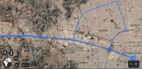
Figure 1. Driver route loop
The data acquisition experiment took place in an urban environment that encompassed a variety of road types. These included express lanes, arterial roads, continuous curved roads, one roundabout, and six signalized intersections. The chosen location provided a diverse range of driving scenarios for data collection. The specific road types and their spatial arrangement within the urban area are visually depicted in Figure 1. This comprehensive selection of road configurations ensures the inclusion of various driving scenarios, allowing for a comprehensive analysis of driver behavior and performance within an urban context. the participants were exposed to identical weather conditions during the testing period. While the specific details of the weather conditions are not mentioned in the provided information, measures were taken to ensure uniformity among participants.
3.1.2 Design and installation of the data acquisition system
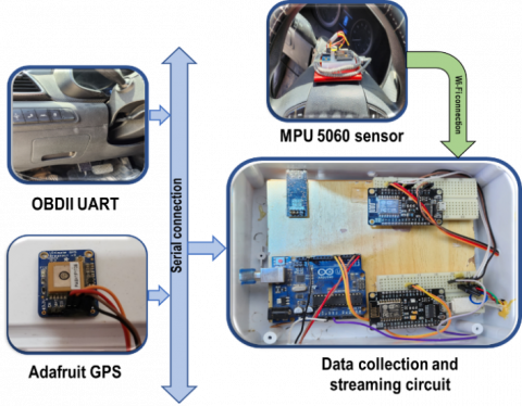
Data collection involved the utilization of three distinct sensor types to gather relevant information. These sensors encompassed the measurement of the accelerator pedal value, throttle position signal, coolant temperature, long-term fuel trim bank 1, and short-term fuel trim bank 1.
Additionally, RPM, speed derived from the OBD-II UART sensor, yaw angle ascertained from the MPU5060 sensor, and vehicle location acquired from the Adafruit GPS breakout were recorded. By incorporating these sensor technologies, a comprehensive dataset was compiled, facilitating the analysis of various vehicle parameters and characteristics. Figure 2 illustrates the physical circuit setup for the in-vehicle sensors, including the OBD-II UART sensor, Adafruit GPS breakout, and MPU5060 sensor. This schematic representation showcases the interconnection and positioning of these sensors within the vehicle. The circuit design ensures the accurate and reliable acquisition of data from these sensors, enabling the collection of essential information for the study.
These sensors were configured to record data at a sampling rate of 1Hz, where the average value of all the data within one second was considered as the representative value for that particular second. Figure 3 provides a visual representation of this data sampling process.
3.1.3 Normalization of features and sample structure
Data preparation is essential of deep learning pipeline, a two-step process of standardization was employed. The first step involved mean subtraction, where the mean value of the data was subtracted from each data point. This process helps center the data around zero, making it easier for the model to learn and converge efficiently. The second step involved division by the standard deviation, which scales the data to have a unit variance. By dividing each data point by the standard deviation, the data was normalized and brought to a common scale, minimizing the impact of varying magnitudes among different features. This standardization process ensures that each feature contributes equally during the training phase, preventing any particular feature from dominating the learning process. By undergoing this two-step data preparation process, the deep learning pipeline was able to handle the input data effectively and improve the model's performance and generalization capabilities.
Figure 2. Physical circuit of in-vehicle sensors
Figure 3. Visual representation of collected data
$\mu=\frac{1}{M} \sum_1^M d_i$ (1)
$\sigma=\sqrt{\frac{\sum_1^M\left(d_i-\mu\right)}{M}}$ (2)
$d_{standardized}=\frac{d_{\text {actual }}-\mu}{\sigma}$ (3)
Eq. (3) outlines the process of standardization, where each data point ($d_{actual}$) is subtracted by the mean (μ) and divided by the standard deviation (σ). This standardization process ensures that the data is transformed to have a mean of 0 and a standard deviation of 1, enabling fair comparisons and analysis across the dataset.
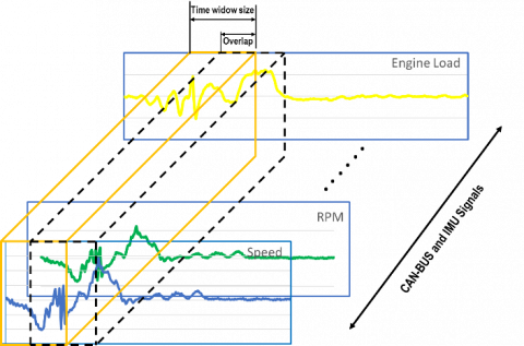
A sliding window approach with a step size of 10 seconds and an overlap window of 9 seconds was applied to the in-vehicle sensor data collected from the OBD-II UART sensor, Adafruit GPS breakout, and MPU5060 sensor. This sliding window technique facilitated the segmentation of the continuous sensor data into smaller, temporally overlapping windows for analysis. By setting the step size to 1 seconds and the overlap window to 9 seconds, a significant portion of the data was shared between adjacent windows, ensuring a comprehensive coverage of the sensor readings as shown in Figure 4. This approach allowed for the extraction of temporal patterns and trends in the sensor data, enabling the investigation of dynamic changes in vehicle performance, location, and orientation over time. It also facilitated the application of various time-series analysis techniques to derive meaningful insights from the collected sensor data.
Figure 4. Overlapping window sliding
3.2 Classification model
Driving datasets can be understood as collections of sequential data points arranged in a time series structure. These time series problems being classified into two categories according to the number of variables involved: univariate time series, which focus on a single variable, and multivariate time series, which incorporate multiple variables. In the context of driving datasets, it is common to have at least four time series features such as speed, acceleration, etc. This suggests that a time series with multiple variables classification issue can be used to frame the challenge of driver categorization. In the subsequent stage of our methodology, the dataset was transformed into a 3-dimintion array structure (features, samples, steps), where features denote the features number, samples represent the samples number in the dataset, and steps corresponds to window size.
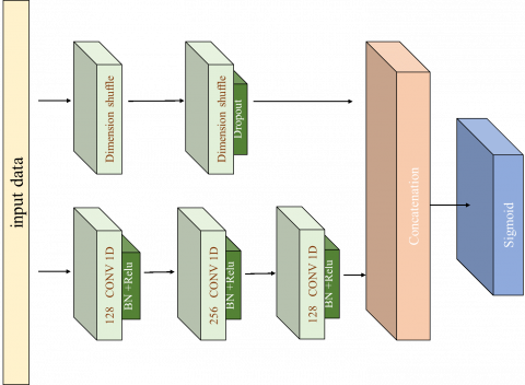
To enhance the classification of time series data, Karim et al. [43] introduced hybrid deep learning model including Fully Convolution network with Long short-term memory (FCN-LSTM) network, as illustrated in Figure 5. By employing the FCN-LSTM architecture, the researchers achieved remarkable improvements and enhanced accuracy across a variety of time series classification challenges with minimum data preprocessing. The FCN-LSTM model combines the strengths of Convolutional Neural Networks (CNNs), which are renowned for their effectiveness in time series classification, with Long Short-Term Memory (LSTM) networks to capture temporal dependencies within the sequences.
In this study, we employing driving data along with FCN-LSTM to classify drivers. Without any previous feature engineering, such as the use of statistical characteristics, the data was simply entered into the model. We can attain an ideal preprocessing time using this approach. Each of these methods, as shown in Figure 5, uses the same data input, but from several angles. The data is delivered to the CNN block as a univariate time series with several time steps. k This change is made to lessen the problem of the data rapidly becoming overfit.
According to Figure 5, the FCN-LSTM architecture incorporates both a fully convolutional block and an LSTM block with dropout, as described in the study [43]. The fully convolutional block comprises three successive temporal convolutional blocks with filter widths of 128, 256, and 128, respectively, following the convolution block structure proposed by Wang et al. [44]. Each convolutional block consists of batch normalization [45], followed by a temporal convolutional layer with a momentum of 0.99 and an epsilon value of 0.001. A ReLU activation function is applied after the convolutional layer. Subsequently, a global average pooling operation is performed after the last convolution block.
Figure 5. FCN-LSTM proposed model
Concurrently, the time series input undergoes a dimension shuffle layer to reorganize its structure. The resulting transformed time series is subsequently fed into the LSTM block, which consist of LSTM layer. A dropout layer is applied after the LSTM block. The output from the global pooling layer and the LSTM block is merged through concatenation and then forwarded to a softmax classification layer.
Long short-term memory networks (LSTMs) have emerged as an advancement over conventional recurrent neural networks, addressing the challenge of vanishing gradients. LSTMs tackle this problem by incorporating memory cells and gating mechanisms that effectively regulate the storage and retrieval of past states. In each time step, an LSTM maintains a hidden vector (h) and a memory vector (m), which play a crucial role in controlling state updates and generating outputs.
The data is divided into 10-time increments, where each increment represents a time series of 10 seconds. The architecture utilizes a dual-branch structure to process the data.
In the first branch, the data is processed through the CNN block. The CNN block treats the data as a univariate time series with multiple time steps.
In the second branch, the data undergoes a dimension shuffle operation before entering the LSTM block. This operation reshapes the data, allowing the LSTM block to interpret it as a multivariate time series. The dimension shuffle layer rearranges the data to be perceived as 10 variables with a single time step. This transformation enables the LSTM block to effectively model temporal dependencies and capture the dynamics of driver behavior over time.
The outputs from both branches, representing the spatial features from the CNN block and the temporal patterns from the reshaped data in the LSTM block, are concatenated. This concatenation integrates the spatial and temporal information in a seamless manner. By combining these components, the FCN-LSTM architecture captures both local spatial features and global temporal dependencies, resulting in a more comprehensive understanding and accurate prediction of driver behavior.
4.1 Experiment setup
To investigate driver behaviour using the FCN-LSTM deep learning model, a dataset was collected specifically for this study. The dataset comprises driving data captured from various sensors and devices installed in vehicles (explained in section 3.1). The collected dataset was divided into training and testing sets using an 80:20 ratio. This means that 80% of the data was allocated for training the FCN-LSTM model, while the remaining 20% was reserved for evaluating its performance. The splitting process was carried out randomly to ensure representative samples in both sets.
To assess the performance of the FCN-LSTM model, various evaluation metrics were utilized. These metrics include accuracy, precision, recall, and F1-score.
Accuracy $=\frac{(\mathrm{TP}+\mathrm{TN})}{(\mathrm{TP}+\mathrm{TN}+\mathrm{FP}+\mathrm{FN})}$ (4)
Precision $=\mathrm{TP} /(\mathrm{TP}+\mathrm{FP})$ (5)
Recall $=\mathrm{TP} /(\mathrm{TP}+\mathrm{FN})$ (6)
$\mathrm{F} 1-$ measure $=\frac{2 ×(\text { Presicsion } × \text { Recall })}{(\text { Presion }+ \text { Recall })}$ (7)
Additionally, confusion matrices were generated to gain insights into the classification results and identify any potential biases or errors.
The deep learning methodologies utilized in this research are extensively elucidated in Table 2. Based on the collected data, the driver behaviour classification techniques employed were evaluated using diverse metrics, and their rankings are presented as follows: FCN-LSTM>1D CNN, LSTM>ANN. The performance results presented in the tables unequivocally indicate that the proposed approach outperforms other existing methodologies. All experiments were conducted moderate performance capabilities equipped with suitable hardware Core (TM) i7-6600U, including GPUs (NVIDIA Quadro M500M), to accelerate the training process. The FCN-LSTM model was implemented using TensorFlow 2.6 as deep learning frameworks.
Table 2. User-defined parameter for proposed model
|
Model |
Parameters |
|
ANN |
3 Layer, 30 neuron |
|
LSTM |
2 Layer, 20 neuron |
|
1D CNN |
3 Layer, 128 units |
4.2 Results and discussion
To assess the performance of our models, we conducted a comparative analysis with several other methods as depicted in Table 2 using the same evaluation metrics.
Furthermore, the FCN-LSTM algorithm emerged as the most effective approach for driver behaviour classification. The proposed technique showcased superior performance across various metrics, such as accuracy, F1-score, and Area under the curve. The evaluation of the four machine learning methods (ANN, CNN, LSTM, FCN-LSTM) according to different window sizes with overlap revealed consistent superiority of the FCN-LSTM model over the other models.
The tables (Tables 3-6) showcase the metric performance of the proposed models for different window sizes-overlap size in seconds: (5-3), (10-5), (10-7), and (10-9). Table 3 reveals the performance of the models for the window size- overlap size of (5-3) seconds. The FCN-LSTM model outperformed the other models with the highest accuracy of 94.39%, an F1 score of 94%, and an impressive AUC of 94.10%.
Moving to Table 4, which represents the metric performance for the window size of (10-5) seconds, we can observe that the FCN-LSTM model again exhibited superior performance. It achieved an exceptional accuracy of 96.23%, an F1 score of 96.00%, and an AUC of 96.16%.
Table 3. The metric performance of the proposed models for window size (5-3) second
|
Model |
Accuracy |
F1 Score |
AUC |
|
ANN |
92.89% |
93.00% |
92.38% |
|
1D CNN |
93.84% |
94.00% |
93.39% |
|
LSTM |
93.16% |
93.00% |
92.62% |
|
FCN-LSTM |
94.39% |
94.00% |
94.10% |
Table 4. The metric performance of the proposed models for window size (10-5) second
|
Model |
Accuracy |
F1 Score |
AUC |
|
ANN |
82.19% |
82% |
81.36% |
|
1D CNN |
92.81% |
93% |
92.34% |
|
LSTM |
93.15% |
93% |
92.86% |
|
FCN-LSTM |
96.23% |
96% |
96.16% |
In Table 5, corresponding to the window size of (10-7) seconds, the FCN-LSTM model continued to demonstrate remarkable performance. It achieved an accuracy of 95.46%, an F1 score of 96.00%, and an AUC of 95.96%. Lastly, Table 6 presents the metric performance for the window size of (10-9) seconds. In this case, the FCN-LSTM model maintained its exceptional performance, achieving a remarkable accuracy of 99.01%, an F1 score of 99.00%, and an AUC of 98.87%.
Table 5. The metric performance of the proposed models for window size (10-7) second
|
Model |
Accuracy |
F1 Score |
AUC |
|
ANN |
91.96% |
92% |
91.59% |
|
1D CNN |
94.02% |
94% |
93.68% |
|
LSTM |
95.88% |
96% |
95.59% |
|
FCN-LSTM |
95.46% |
96% |
95.96% |
Table 6. The metric performance of the proposed models for window size (10-9) second
|
Model |
Accuracy |
F1 Score |
AUC |
|
ANN |
92.02% |
92% |
91.55% |
|
1D CNN |
98.42% |
98% |
98.28% |
|
LSTM |
96.77% |
97% |
96.65% |
|
FCN-LSTM |
99.01% |
99% |
98.87% |
Overall, the tables demonstrate that the FCN-LSTM model consistently outperformed other models across different window sizes. It achieved higher accuracy, F1 score, and AUC values, indicating its effectiveness in accurately classifying driver behaviour. These findings highlight the superiority of the FCN-LSTM model over alternative approaches, underscoring its potential for real-world driver behaviour classification tasks.
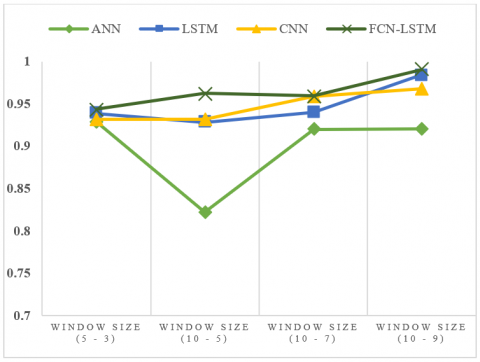
Figure 6. FCN-LSTM proposed model
The accuracy of the proposed models exhibits variation across different window sizes and overlaps. Figure 6 depicts the accuracy curves for the proposed models (ANN, LSTM, CNN, FCN-LSTM) for four distinct window sizes. For the initial window size of (5-3) seconds, the proposed models achieve a notably high accuracy level. However, as the window size increases to 10 seconds while reducing the overlap to 50%, the accuracy tends to decrease. Conversely, for the third window size, where the overlap increases to 7 seconds, the accuracy shows improvement. These findings emphasize the influence of window size and overlap on the accuracy of the models. Notably, the models demonstrate the highest accuracy when the overlap size is 9 seconds, representing 90% of the signal. However, Smaller window sizes capture fine-grained details, while larger window sizes capture long-term dependencies. Higher overlaps enhance temporal context, while reduced overlaps may limit contextual information.
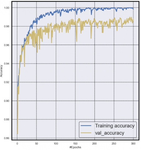
Figure 7. Accuracy learning curve of the FCN-LSTM
Figure 7 illustrating the training accuracy and validation accuracy for the FCN-LSTM model with a window size of (10-9) seconds over 300 epochs provids valuable insights into the model's performance throughout the training process. The training accuracy curve represents the accuracy achieved by the model on the training dataset at each epoch. It shows how well the model is learning from the training data over time. The validation accuracy curve, on the other hand, illustrates the accuracy of the model on a separate validation dataset at each epoch. The validation dataset serves as a benchmark to evaluate the model's generalization and performance on unseen data.
4.3 Robustness to data anomalies
The accuracy of driver behaviour heavily depends on the reliability of car sensor data. However, sensors are vulnerable to malfunctions, failures, and potential hacking, which can introduce inaccuracies and abnormal data into the model. This can result in incorrect predictions. To address this challenge, it is important for a driver behaviour system to incorporate mechanisms that can effectively detect and correct anomalies, ensuring accurate predictions. To evaluate the model's performance in the presence of anomalies, a proposed robustness analysis aims to assess its ability to maintain accurate predictions even when anomalous data is present.
Table 7. The metric performance of the proposed models for window size (10-9) second
|
Anomaly Rate |
Anomaly Duration |
ANN |
LSTM |
1DCNN |
FCN-LSTM |
|
0% |
1 s |
92.30 |
96.56 |
98.14 |
99.01 |
|
10 s |
92.30 |
96.56 |
98.14 |
99.01 |
|
|
1% |
1 s |
92.23 |
96.42 |
97.94 |
98.35 |
|
10 s |
92.09 |
96.56 |
98.07 |
98.35 |
|
|
10% |
1 s |
91.40 |
96.01 |
97.66 |
98.14 |
|
10 s |
90.92 |
95.46 |
97.11 |
98.28 |
|
|
30% |
1 s |
89.82 |
95.39 |
95.74 |
97.04 |
|
10 s |
89.89 |
93.33 |
95.74 |
97.04 |
|
|
50% |
1 s |
87.83 |
94.91 |
93.67 |
95.19 |
|
10 s |
86.73 |
90.44 |
93.74 |
94.43 |
To conduct our analysis, we select a subset of random sensors from a total of 12 features for modification. In this case, we choose 7 sensors to be modified. We simulate different rates of anomalies, specifically 1%, 10%, 30% and 50% of the total samples from the validation set. For each rate, we introduce random values into the selected 7 features, thereby modifying the data. Additionally, we simulate two different anomaly durations, namely 1 second and 10 seconds. The performance of the FCN-LSTM model surpasses that of the other models consistently across various anomaly rates and durations, as demonstrated in Table 7. It attains the highest accuracy in the majority of cases, indicating its superior performance compared to the alternative models.
This paper highlights the significant promise and potential of driver behavior classification using deep learning models with in-vehicle data. The utilization of deep learning models such as ANN, LSTM, CNN, and FCN-LSTM has demonstrated high accuracy in analyzing and classifying driver behavior by leveraging the rich information captured by in-vehicle sensors. These models extract meaningful patterns and features from sensors like accelerometers, gyroscopes, and GPS data. However, certain challenges remain in this field, including ensuring data privacy and security, addressing the interpretability of deep learning models, and promoting their explain ability. Additionally, the generalization of models across diverse driving scenarios and the scalability of real-time applications requires further investigation. Despite these challenges, driver behavior classification based on deep learning with in-vehicle data has showcased promising results. The advancements in driver behavior classification using deep learning models have the potential for significant real-world impact. Firstly, they can greatly enhance driver safety by providing insights into driver behavior patterns and identifying risky behaviors. Moreover, these models can contribute to the development of intelligent transportation systems by enabling a deeper understanding of driver behavior in various driving scenarios. Continued research and development in this area will drive further advancements and practical applications in the analysis of driver behavior.
[1] Yang, S., Kuo, J., Lenné, M.G. (2021). Effects of distraction in on-road level 2 automated driving: Impacts on glance behavior and takeover performance. Human Factors, 63(8): 1485-1497. https://doi.org/10.1177/0018720820936793
[2] Morgenstern, T., Wögerbauer, E.M., Naujoks, F., Krems, J.F., Keinath, A. (2020). Measuring driver distraction-Evaluation of the box task method as a tool for assessing in-vehicle system demand. Applied Ergonomics, 88: 103181. https://doi.org/10.1016/j.apergo.2020.103181
[3] McDonald, A.D., Ferris, T.K., Wiener, T.A. (2020). Classification of driver distraction: A comprehensive analysis of feature generation, machine learning, and input measures. Human Factors, 62(6): 1019-1035. https://doi.org/10.1177/0018720819856454
[4] Box, S. (2006). Transportation institute releases findings on driver behavior and crash factors.
[5] Obregón-Biosca, S.A., Romero-Navarrete, J.A., Betanzo-Quezada, E. (2018). Traffic crashes probability: A socioeconomic and educational approach. Transportation Research Part F: Traffic Psychology and Behaviour, 58: 619-628. https://doi.org/10.1016/j.trf.2018.06.041
[6] Nowosielski, R.J., Trick, L.M., Toxopeus, R. (2018). Good distractions: Testing the effects of listening to an audiobook on driving performance in simple and complex road environments. Accident Analysis & Prevention, 111: 202-209. https://doi.org/10.1016/j.aap.2017.11.033
[7] Abou Elassad, Z.E., Mousannif, H., Al Moatassime, H., Karkouch, A. (2020). The application of machine learning techniques for driving behavior analysis: A conceptual framework and a systematic literature review. Engineering Applications of Artificial Intelligence, 87: 103312. https://doi.org/10.1016/j.engappai.2019.103312
[8] Shahar, M.S.M., Mazalan, L. (2021). Face identity for face mask recognition system. In 2021 IEEE 11th IEEE Symposium on Computer Applications & Industrial Electronics (ISCAIE), pp. 42-47. https://doi.org/10.1109/ISCAIE51753.2021.9431791
[9] Li, M., Xu, H., Huang, X., Song, Z., Liu, X., Li, X. (2018). Facial expression recognition with identity and emotion joint learning. IEEE Transactions on Affective Computing, 12(2): 544-550. https://doi.org/10.1109/TAFFC.2018.2880201
[10] Ali, K., Hughes, C.E. (2021). Facial expression recognition by using a disentangled identity-invariant expression representation. In 2020 25th International Conference on Pattern Recognition (ICPR), IEEE, pp. 9460-9467. https://doi.org/10.1109/ICPR48806.2021.9412172
[11] Cheng, A.L., Bier, H., Latorre, G. (2018). Actuation confirmation and negation via facial-identity and-expression recognition. In 2018 IEEE Third Ecuador Technical Chapters Meeting (ETCM), pp. 1-6. https://doi.org/10.1109/ETCM.2018.8580319
[12] Chen, J., Chen, J., Wang, Z., Liang, C., Lin, C.W. (2020). Identity-aware face super-resolution for low-resolution face recognition. IEEE Signal Processing Letters, 27: 645-649. https://doi.org/10.1109/LSP.2020.2986942
[13] Yang, H., Zhang, Z., Yin, L. (2018). Identity-adaptive facial expression recognition through expression regeneration using conditional generative adversarial networks. In 2018 13th IEEE International Conference on Automatic Face & Gesture Recognition (FG 2018), pp. 294-301. https://doi.org/10.1109/FG.2018.00050
[14] Li, Z., Niu, Z., Kuang, G., Li, P. (2020). Living identity verification via dynamic face-speech recognition. In 2020 Information Communication Technologies Conference (ICTC), IEEE, pp. 265-271. https://doi.org/10.1109/ICTC49638.2020.9123311
[15] Wei, J., Wang, Y., Li, Y., He, R., Sun, Z. (2021). Cross-spectral iris recognition by learning device-specific band. IEEE Transactions on Circuits and Systems for Video Technology, 32(6): 3810-3824. https://doi.org/10.1109/TCSVT.2021.3117291
[16] Eisenman, S.B., Miluzzo, E., Lane, N.D., Peterson, R.A., Ahn, G.S., Campbell, A.T. (2010). BikeNet: A mobile sensing system for cyclist experience mapping. ACM Transactions on Sensor Networks (TOSN), 6(1): 1-39. https://doi.org/10.1145/1653760.1653766
[17] Khan, M.Q., Lee, S. (2019). A comprehensive survey of driving monitoring and assistance systems. Sensors, 19(11): 2574. https://doi.org/10.3390/s19112574
[18] Pentland, A., Liu, A. (1999). Modeling and prediction of human behavior. Neural Computation, 11(1): 229-242. https://doi.org/10.1162/089976699300016890
[19] Al-Hussein, W.A., Kiah, M.L.M., Por, L.Y., Zaidan, B.B. (2021). Investigating the effect of social and cultural factors on drivers in Malaysia: A naturalistic driving study. International Journal of Environmental Research and Public Health, 18(22): 11740. https://doi.org/10.3390/ijerph182211740
[20] Li, Z., Zhang, K., Chen, B., Dong, Y., Zhang, L. (2019). Driver identification in intelligent vehicle systems using machine learning algorithms. IET Intelligent Transport Systems, 13(1): 40-47. https://doi.org/10.1049/iet-its.2017.0254
[21] Alsrehin, N.O., Klaib, A.F., Magableh, A. (2019). Intelligent transportation and control systems using data mining and machine learning techniques: A comprehensive study. IEEE Access, 7: 49830-49857. https://doi.org/10.1109/ACCESS.2019.2909114
[22] Carmona, J., de Miguel, M.A., Martin, D., Garcia, F., de la Escalera, A. (2016). Embedded system for driver behavior analysis based on GMM. In 2016 IEEE Intelligent Vehicles Symposium (IV), pp. 61-65. https://doi.org/10.1109/IVS.2016.7535365
[23] Ferreira, J., Carvalho, E., Ferreira, B.V., de Souza, C., Suhara, Y., Pentland, A., Pessin, G. (2017). Driver behavior profiling: An investigation with different smartphone sensors and machine learning. PLoS One, 12(4): e0174959. https://doi.org/10.1371/journal.pone.0174959
[24] Shahverdy, M., Fathy, M., Berangi, R., Sabokrou, M. (2020). Driver behavior detection and classification using deep convolutional neural networks. Expert Systems with Applications, 149: 113240. https://doi.org/10.1016/j.eswa.2020.113240
[25] McNew, J.M. (2012). Predicting cruising speed through data-driven driver modeling. In 2012 15th International IEEE Conference on Intelligent Transportation Systems, pp. 1789-1796. https://doi.org/10.1109/ITSC.2012.6338762
[26] Chen, D., Cho, K.T., Shin, K.G. (2017). Mobile IMUs reveal driver's identity from vehicle turns. arXiv Preprint arXiv: 1710.04578. https://doi.org/10.48550/arXiv.1710.04578
[27] Li, Y., Miyajima, C., Kitaoka, N., Takeda, K. (2015). Evaluation method for aggressiveness of driving behavior using drive recorders. IEEJ Journal of Industry Applications, 4(1): 59-66. https://doi.org/10.1541/ieejjia.4.59
[28] Lee, J., Jang, K. (2019). A framework for evaluating aggressive driving behaviors based on in-vehicle driving records. Transportation Research Part F: Traffic Psychology and Behaviour, 65: 610-619. https://doi.org/10.1016/j.trf.2017.11.021
[29] Zylius, G. (2017). Investigation of route-independent aggressive and safe driving features obtained from accelerometer signals. IEEE Intelligent Transportation Systems Magazine, 9(2): 103-113. https://doi.org/10.1109/MITS.2017.2666583
[30] Choi, G., Lim, K., Pan, S.B. (2022). Driver identification system using 2D ECG and EMG based on multistream CNN for intelligent vehicle. IEEE Sensors Letters, 6(6): 1-4. https://doi.org/10.1109/LSENS.2022.3175787
[31] Hong-yu, H.U., Jia-rui, L.I.U., Fei, G.A.O., Zhen-hai, G.A.O., Xing-tai, M.E.I., Guang, Y.A.N.G. (2020). Driver identification based on 1-D convolutional neural networks. China Journal of Highway and Transport, 33(8): 195.
[32] Al-Hussein, W.A., Por, L.Y., Kiah, M.L.M., Zaidan, B.B. (2022). Driver behavior profiling and recognition using deep-learning methods: In accordance with traffic regulations and experts guidelines. International Journal of Environmental Research and Public Health, 19(3): 1470. https://doi.org/10.3390/ijerph19031470
[33] Aslan, C., Genç, Y. (2021). Driver identification using vehicle diagnostic data with fully convolutional neural network. In 2021 29th Signal Processing and Communications Applications Conference (SIU), IEEE, pp. 1-4. https://doi.org/10.1109/SIU53274.2021.9477850
[34] Chen, J., Wu, Z., Zhang, J. (2019). Driver identification based on hidden feature extraction by using adaptive nonnegativity-constrained autoencoder. Applied Soft Computing, 74: 1-9. https://doi.org/10.1016/j.asoc.2018.09.030
[35] Alatabani, L.E., Ali, E.S., Saeed, R.A. (2021). Deep learning approaches for IoV applications and services. In Intelligent Technologies for Internet of Vehicles. Cham: Springer International Publishing, pp. 253-291. https://doi.org/10.1007/978-3-030-76493-7_8
[36] Morton, J., Wheeler, T.A., Kochenderfer, M.J. (2016). Analysis of recurrent neural networks for probabilistic modeling of driver behavior. IEEE Transactions on Intelligent Transportation Systems, 18(5): 1289-1298. https://doi.org/10.1109/TITS.2016.2603007
[37] Carvalho, E., Ferreira, B.V., Ferreira, J., De Souza, C., Carvalho, H.V., Suhara, Y., Pentland, A.S., Pessin, G. (2017). Exploiting the use of recurrent neural networks for driver behavior profiling. In 2017 International Joint Conference on Neural Networks (IJCNN), IEEE, pp. 3016-3021. https://doi.org/10.1109/IJCNN.2017.7966230
[38] Chen, M., Tian, Y., Fortino, G., Zhang, J., Humar, I. (2018). Cognitive internet of vehicles. Computer Communications, 120: 58-70. https://doi.org/10.1016/j.comcom.2018.02.006.
[39] Al-Rakhami, M.S., Gumaei, A., Hassan, M.M., Alamri, A., Alhussein, M., Razzaque, M.A., Fortino, G. (2021). A deep learning-based edge-fog-cloud framework for driving behavior management. Computers & Electrical Engineering, 96: 107573. https://doi.org/10.1016/j.compeleceng.2021.107573
[40] Alamri, A., Gumaei, A., Al-Rakhami, M., Hassan, M.M., Alhussein, M., Fortino, G. (2020). An effective bio-signal-based driver behavior monitoring system using a generalized deep learning approach. IEEE Access, 8: 135037-135049. https://doi.org/10.1109/ACCESS.2020.3011003
[41] Ma, Y., Li,W., Tang, K., Zhang, Z., Chen, S. (2021). Driving style recognition and comparisons among driving tasks based on driver behavior in the online car-hailing industry. Accident Analysis & Prevention, 154: 106096. https://doi.org/10.1016/j.aap.2021.106096
[42] Andria, G., Attivissimo, F., Di Nisio, A., Lanzolla, A.M.L., Pellegrino, A. (2016). Development of an automotive data acquisition platform for analysis of driving behavior. Measurement, 93: 278-287. https://doi.org/10.1016/j.measurement.2016.07.035
[43] Karim, F., Majumdar, S., Darabi, H., Chen, S. (2017). LSTM fully convolutional networks for time series classification. IEEE Access, 6: 1662-1669. https://doi.org/10.1109/ACCESS.2017.2779939
[44] Wang, Z.G., Yan, W.Z., Oates, T. (2017). Time series classification from scratch with deep neural networks: A strong baseline. 2017 International Joint Conference on Neural Networks (IJCNN), Anchorage, USA, pp. 1578-1585. https://doi.org/10.1109/IJCNN.2017.7966039.
[45] Ioffe, S., Szegedy, C. (2015). Batch normalization: Accelerating deep network training by reducing internal covariate shift. In International conference on machine learning, pp. 448-456.