Lili Yang
OPEN ACCESS
The optimal control inputs obtained by the traditional robot motion optimization methods are nonzero at the start and end of robot motion, making it difficult to control the attitude motion of the robot directly with the motor. To solve the problem, this paper combines the particle swarm optimization (PSO) with spline approximation into a new method, which can replace the Fourier approximation in traditional algorithm. Firstly, the author set up the dynamic model of the system, and transformed the motion planning problem with nonholonomic constraints into the optimal control problem, under the conservation of angular momentum. Next, the spline approximation and the PSO were employed to optimize the trajectory of the attitude motion of the system, and control the inputs to zero at the start and end of robot motion, such that the robot could move from the initial position to the desired destination in a motion cycle. The proposed algorithm was proved through numerical experiment as capable of effectively controlling the attitude motion of nonholonomic hopping robot.
one-legged hopping robot, nonholonomic constraint, attitude motion planning, spline approximation, particle swarm optimization (PSO)
With the continuous development of robotics, the working environment of robots has become increasingly diverse and complex. The traditional fixed-point operations in simple environment are gradually being replaced by autonomous operations in non-structured environments, such as space exploration, archaeological exploration and geological exploration.
The motions of mobile robots [1] mainly include: wheeled or tracklaying motion, bionic crawling or walking, and hopping. Among them, hopping is the most suitable motion in complex or unknown working environments. A hopping robot can get across large obstacles several times its height, making it an ideal substitute for human. In addition, the hopping robot enjoys unique advantages in specific environments like microgravity space. Hopping can expand the radius and range of motion, and save more energy than other motions. Therefore, hopping robot boasts better adaptivity to various environments than other kinds of robots [2].
When moving in the air, a hopping robot obeys the conservation of angular momentum and thus faces several nonholonomic constraints, which may also arise if the contact between rigid bodies is not sliding or rolling [3]. In this case, the attitude control of the robot becomes a typical nonholonomic motion problem [4]. The nonholonomic features of the robot system are resulted from the non-integral angular velocity. Specifically, the dimension number of the generalized coordinates of the system is more than that of the control input, and the nonholonomic constraints cannot be expressed as the constraint form of configuration space by integration.
The nonholonomic system is a special nonlinear system. The motion control of such a system is more difficult than that in general systems, and has become a research hotspot in recent years [5-7]. Some scholars have attempted to optimize the trajectory and control law of robot motion with optimization methods like Fourier approximation, Ritz approximation and variable structure control. For example, Yang (2013) [8] designed numerical algorithms for attitude motion control based on several optimization strategies (i.e. particle swarm optimization (PSO), genetic algorithm (GA) and quasi newton algorithm), and obtained the optimal trajectory and control law of the robot system. However, the optimal control inputs obtained by the above methods are nonzero at the start and end of robot motion. Thus, it is difficult to control the attitude motion of the robot directly with the motor.
To solve the problem, this paper combines the PSO with spline approximation into a new method, which can replace the Fourier approximation in traditional algorithm. Firstly, the author set up the dynamic model of the system, and transformed the motion planning problem with nonholonomic constraints into the optimal control problem, under the conservation of angular momentum. Next, the spline approximation and the PSO were employed to optimize the trajectory of the attitude motion of the system, and control the inputs to zero at the start and end of robot motion, such that the robot could move from the initial position to the desired destination in a motion cycle. The proposed algorithm was proved through numerical experiment as capable of effectively controlling the attitude motion of nonholonomic hopping robot.
Figure 1. Model of one-legged hopping robot
Our hopping robot system consists of a body and a leg that can rotate and flex freely. Without considering the flexible deformation, the author attempted to build a rigid model for the robot system. As shown in Figure 1, the robot has 2 degrees-of-freedom (DOFs), i.e. capable of moving in the plane. According to the theory of dynamics of multi-body system, the mobile robot obeys the conservation of angular momentum in the absence of external force or moment. The angular momentum of the robot can be expressed as [2]:
$\mathrm{I\dot{ }\!\!\theta\!\!\text{ }+m(l+d}{{\mathrm{)}}^{\mathrm{2}}}\mathrm{(\dot{ }\!\!\theta\!\!\text{ }+\dot{ }\!\!\psi\!\!\text{ })}$ (1)
where I is the inertial matrix of the body; m is the mass of the leg (assumed to concentrate on the foot); d is the upper leg length; ψ is the rotation angle of the leg relative to the body; l is the flex quanity of the leg; θ is the rotation angle of the body. ψ, l and θ are collectively known as the configuration parameters of the robot, q=(ψ,l,θ).
Since the initial angular momentum of the robot is zero, the following can be derived from formula (1):
$\mathrm{I\dot{ }\!\!\theta\!\!\text{ }+m(l+d}{{\mathrm{)}}^{\mathrm{2}}}\mathrm{(\dot{ }\!\!\theta\!\!\text{ }+\dot{ }\!\!\psi\!\!\text{ })=0}$ (2)
Formula (2) can be considered as Pfaffian constraints expressed by the three generalized velocities of the system, $\dot{ψ}$, $\dot{l}$ and $\dot{θ}$. As the basis of the constrained 2D zero space, two vector fields $\dot{ψ}=u_1$ and $\dot{l}=u_2$ corresponding to the ψ and l of the leg can be taken as the control inputs of the system. In this way, the change law of the three configuration parameters are controlled by two control inputs when the robot moves in the plane. Substituting $\dot{ψ}=u_1$ and $\dot{l}=u_2$ into formula (2), we have:
$\mathrm{\dot{q}=B(q)u}$ (3)
where $B\mathrm{(}q\mathrm{)=}\left[ \begin{align} & \begin{matrix} \mathrm{1} & \mathrm{0} \\\end{matrix} \\ & \begin{matrix} \mathrm{0} & \mathrm{1} \\\end{matrix} \\ & \begin{matrix} \mathrm{-}\frac{\mathrm{m(l+d}{{\mathrm{)}}^{\mathrm{2}}}}{\mathrm{I+m(l+d}{{\mathrm{)}}^{\mathrm{2}}}} & \mathrm{0} \\\end{matrix} \\\end{align} \right]$; $u\mathrm{=}\left[ \begin{matrix} {\mathrm{\dot{ }\!\!\Psi\!\!\text{ }}} \\ {\mathrm{\dot{l}}} \\\end{matrix} \right]$.
Derived from the system’s conservation of angular momentum, formula (3) exists in the integrable form. In other words, the one-legged hopping robot system is constrained by an integrable angular velocity, a typical nonholonomic constraint [9]. The motion state q in the motion-time horizon can be obtained by formula (3), which is integrated with the adaptive fourth-order-Runge-Kutta method.
Formula (3) provides a function of q relative to u and t. In fact, this formula specifies the attitude motion of a one-legged hopping robot (three configuration parameters) under two control inputs. Under nonholonomic constraint, the common goal of motion planning is to find the control input u such that the system moves from a given initial position $q_0=(ψ_0,l_0,θ_0 )^T∈R^3$ to the desired destination $q_f=(ψ_f,l_f,θ_f )^T∈R^3$ over a specific period of time T, consuming the minimal energy [10]. The optimal law of control input $u(t)∈R^2,t∈[0,T]$ can be obtained by optimizing the objective function.
The attitude motion of the robot is an energy-consuming process. The smoother the change of attitude motion, the less the energy consumption [11]. Considering the above, the minimal energy consumption can be selected as the objective of the optimization:
$J(u)\mathrm{=}\int_{\mathrm{0}}^{\mathrm{T}}{\mathrm{}u,u\mathrm{dt}}$ (4)
where, $u(t)∈L_2([0, T])$ is the set of square integrable functions in [0,T]. The value of $u(t)=[u_1(t),⋯,u_n(t)]^T$ is traditionally determined by Fourier base functions. The results are measurable vector functions in Hilbert Spaces. Here, the value is obtained by spline approximation instead. To be specific, the author employed the cubic spline interpolation, which is the most popular way of piecewise-polynomial approximation [12]. This method is continuously differentiable on the interval and has a continuous second derivative.
For a set of nodes $0=t_0<t_1<⋯<t_N=T$, the cubic spline function s(t_i) on each sub-interval can be established. Then, we have $s(t_i)=u_i (i=1,2,⋯,N-1)$ at the interval nodes, with $u_i$ being the components corresponding to the control input at the interval nodes. Under the boundary conditions $s^″ (0)=0$ and $s^″ (T)=0$, the following can be obtained by natural cubic spline interpolation:
$u\text{(}t\text{)=}s\text{(}\lambda ,t\text{)}, t\in [0,T]$ (5)
where $λ=[u_0,u_1,⋯,u_N ]^T$ are the control input vectors in [0,T]. Substituting formula (5) into formula (4), the objective function of the robot system can be obtained. Then, the control input vector λ can be regarded as a new control variable.
Considering the accuracy constraints on the system motion to the destination, formula (4) can be rewritten as follows with the introduction of a penalty function:
$\mathbf{J}\text{(}\lambda ,\mu \text{)}=\int_{0}^{T}{{{[s(\lambda ,t)]}^{2}}\text{d}t}+\mu \,{{\left\| f(\lambda )-{{q}_{f}} \right\|}^{2}}$ (6)
where μ>0 is the penalty factor; f(λ) is the final position of the robot determined by formula (3) after a set of control inputs u(t) is inputted into that formula. Therefore, the search for the u that minimizes the value of formula (4) can be converted into the search for the λ that minimizes the value of formula (6). Through the above analysis, the attitude motion planning problem of the hopping robot under nonholonomic constraints was transformed into the problem of minimizing formula (6).
In this chapter, the PSO is applied to the attitude motion planning of the robot system. As an evolutionary computing technique, the PSO is a population-based algorithm mimicking the social behaviors of animals, such as fish schooling and bird flocking. By this method, the objective function does not have to be differentiable, and the global optimum of nonlinear optimization problems can be obtained rapidly.
During the implementation of the PSO, each alternative solution is considered as a particle. A number of particles constitute a population that looks for the optimal solution in the search space. The position of each particle should be optimized to track the optimal position of the current population. Meanwhile, each particle has a velocity that determines the direction and distance of its flight. In practical applications, the initial position and velocity of each particle are randomly generated, and the optimal solution of the whole population is searched in the solution space iteratively.
Let D be the number of dimensions of each particle, $X_i=(x_{i1},x_{i2},...,x_{iD})$ be the position vector of particle i, and $V_i=(v_{i1},v_{i2},...,v_{iD}$ be the velocity vector of particle i. In each iteration, each particle updates itself by tracking the local best-known value $P_i$ and the global best-known value $P_g$. The position and velocity of each particle can be updated by [13]:
$\begin{align} & {{V}_{id}}(t+1)=w\cdot {{v}_{id}}(t)+{{c}_{1}}\cdot {{r}_{1}}\cdot [{{P}_{id}}(t)-{{x}_{id}}(t)]+ \\ & {{c}_{2}}\cdot {{r}_{2}}\cdot [{{P}_{gd}}(t)-{{x}_{id}}(t)] \\\end{align}$ (7)
${{X}_{\mathrm{id}}}(\mathrm{t+1})\mathrm{=}{{x}_{\mathrm{id}}}(\mathrm{t})\mathrm{+}{{v}_{\mathrm{id}}}(\mathrm{t+1})$ (8)
where w is inertial value; c1 and c2 are acceleration factors; r1 and r2 are two random numbers uniformly distributed in the interval [0, 1]. The position and velocity of a particle in the dimension d(1≤d≤D) have fixed value ranges. If either parameter exceeds its corresponding range, the boundary value should be taken.
The PSO algorithm is implemented through the following steps:
(1) Initialization
Under the given parameters w, c1, c2, r1 and r2, the position $X_i$ and velocity $V_i$ of each particle are initialized. The local best-known value $P_i$ and the global best-known value $P_g$ are calculated and recorded. The objective function value of each particle is calculated according to formula (6).
(2) Iteration
The position and velocity of each particle are iterated and updated by formulas (7) and (8), respectively.
(3) Judgment
If better than that before the update, the new objective function value of a particle should be adopted. If better than those before the update, the new $P_i$ and $P_g$ should be adopted.
(4) Testing
The program should be terminated and the optimal solution should be recorded, if the maximum number of iterations is reached; otherwise, return to Step (2) and start the next iteration.
The PSO algorithm for one-legged hopping robot motion planning was verified through the simulation of a planar moving robot. The mass and geometric parameters of the robot were set as: $I=16.66kg⋅m^2$, $m=10kg$, $l=0.5m$ and $d=0.5m$.
The parameters of the PSO [14] were initialized as: particle number n=15, acceleration factor $c_1=c_2=1.494$, inertial value w=0.9~0.4, and the number of iterations=500. The particle number was set to 15, because the simulation result will remain the same if there are more than 15 particles.
The motion parameters were defined as follows. The motion time T=5s was divided into five equal parts. The control inputs at the start and end of motion were both set to zero. The number of parameters for each control input was set to 4. The dimension of λ corresponding to two control inputs was set to 8, that is, the dimension of the particle is D=8 when the PSO is applied.
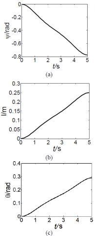
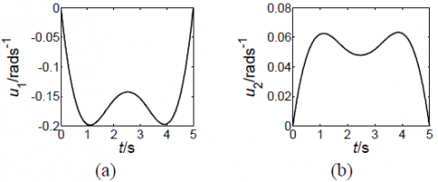
The simulation experiment was carried out on Matlab software. The initial and final coordinates of the robot were assumed to be $[0 0 0)]^T$ and $[-(π/4 0.25 π/12)]^T$, respectively. The simulation results are displayed in Figures 2 and 3.
Figure 2. Motion trajectories of robot configuration parameters
Figure 3. Optimal control input law of robot motion
The above figures show that the trajectory of the robot, as well as the angular velocity and expansion linear velocity of the leg, were all smooth and continuous. Besides, the initial and final velocities were both zero.
In engineering, the motor control of robot attitude motion requires the initial and final control inputs to be zero. However, the common optimization methods like Fourier approximation cannot guarantee the control inputs are zero at the start and end of the robot motion. To solve the problem, this paper combines spline approximation and the PSO into a novel algorithm, and uses it to solve the optimal control problem of attitude motion planning for a hopping robot system under nonholonomic constraints. The proposed algorithm can optimize the motion trajectory of the robot, eliminating the nonzero initial and final values of the control inputs. The algorithm inherits the advantages of the PSO, such as simple structure, limited number of parameters, ease of programming and fast convergence. The research findings shed new light on solving motion control problems of nonholonomic systems.
This work was supported by Zibo science and technology development plan (2016kj010057).
[1] Khaksar, W., Vivekananthen, S., Saharia, K.S.M., Yousefi, M., Ismail, F.B. (2015). A review on mobile robots motion path planning in unknown environments. 2015 IEEE International Symposium on Robotics and Intelligent Sensors (IRIS), pp. 295-300. http://dx.doi.org/10.1109/IRIS.2015.7451628
[2] Raibert, M.H. (2007). Legged robots that balance. IEEE Expert, 1(4): 89-89. http://dx.doi.org/10.1109/MEX.1986.4307016
[3] Bazzi, S., Shammas, E., Asmar, D. (2014). A novel method for modeling skidding for systems with nonholonomic constraints. Nonlinear Dynamics, 76(2): 1517-1528. https://doi.org/10.1007/s11071-013-1225-9
[4] Khan, M.U., Shuai, L., Wang, Q., Shao, Z. (2016). Formation control and tracking for co-operative robots with non-holonomic constraints. Journal of Intelligent & Robotic Systems, 82(1): 163-174. https://doi.org/10.1007/s10846-015-0287-y
[5] Saska, M., Spurný, V., Vonásek, V. (2016). Predictive control and stabilization of nonholonomic formations with integrated spline-path planning. Robotics & Autonomous Systems, 75: 379-397. https://doi.org/10.1016/j.robot.2015.09.004
[6] Roozegar, M., Mahjoob, M.J., Jahromi, M. (2016). Optimal motion planning and control of a nonholonomic spherical robot using dynamic programming approach: simulation and experimental results. Mechatronics, 39: 174-184. https://doi.org/10.1016/j.mechatronics.2016.05.002
[7] Fareh, R., Rabie, T. (2016). Tracking trajectory for nonholonomic mobile manipulator using distributed control strategy. International Symposium on Mechatronics & Its Applications. https://doi.org/10.1109/ISMA.2015.7373473
[8] Yang, L.L. (2013). The numerical method to nonholonomic motion planning of a hopping robot. Manufacturing Automation, 50: 545-553. https://doi.org/10.3969/j.issn.1009-0134.2013.13.026
[9] Janiak, M., Tchoń, K. (2011). Constrained motion planning of nonholonomic systems. Systems & Control Letters, 60(8): 625-631. https://doi.org/10.1016/j.sysconle.2011.04.022
[10] Wu, J.W., Shi, S.C., Liu, H., Cai, H.G. (2011). Spacecraft attitude disturbance optimization of space robot in target capturing process. Robot, 33(1): 16-21. https://doi.org/10.3724/SP.J.1218.2011.00016
[11] Su, P., He, G.P., Xu, M. (2012). Research on motion simulation of hopping robot based on minimum energy-loss principle. Machinery Design & Manufacture, 4: 171-173. https://doi.org/10.3969/j.issn.1001-3997.2012.04.064
[12] Yaghoobi, S., Moghaddam, B.P., Ivaz, K. (2017). An efficient cubic spline approximation for variable-order fractional differential equations with time delay. Nonlinear Dynamics, 87(2): 815-826. https://doi.org/10.1007/s11071-016-3079-4
[13] Poli, R., Kennedy, J., Blackwell, T. (2007). Particle swarm optimization. Swarm Intelligence, 1(1): 33-57. https://doi.org/10.1007/s11721-007-0002-0
[14] Venter, G., Sobieszczanski-Sobieski, J. (2012). Particle Swarm Optimization. 9-th Aiaa/usaf/nasa/issmo Symposium on Multidisciplinary Analysis & Optimization Conference, 41(8): 1583-1585 https://doi.org/10.2514/2.2111