Rania O. Al-Sadi*![]() | Abdul-Sattar J. Al-Saif
| Abdul-Sattar J. Al-Saif![]()
© 2023 IIETA. This article is published by IIETA and is licensed under the CC BY 4.0 license (http://creativecommons.org/licenses/by/4.0/).
OPEN ACCESS
This study introduces a novel method aimed at deriving approximate solutions for diffusive prey-predator systems. The proposed method seeks to circumvent the limitations of extant techniques, which frequently grapple with obtaining accurate analytical solutions and managing intricate computational operations. This new approach amalgamates the Shehu transformation, Akbari-Ganji’s method, and Padé Approximant to facilitate a more precise and efficient solution. The accuracy, efficiency, and effectiveness of the proposed method are assessed through the analysis of two exemplar cases in one- and two-dimensional spaces. Results gleaned from the novel method underscore its superior accuracy and efficiency compared to traditional methods used for approximating analytical solutions to similar problems. Further, the utilization of infographics and tables elucidates the significance, validity, and indispensability of the proposed approach. This research augments our comprehension of biological systems and their interactions with the environment, thereby presenting a valuable contribution to the academic discourse.
Shehu transformation, Akbari -Ganji’s method, Padé approximant, diffusive prey-predator systems, convergence, stability
Predator-prey dynamics form the cornerstone of vibrant ecosystems, with the relationship between predator and prey constituting a pivotal interaction among the various interspecies partnerships in ecology. Differential equation-based mathematical models are typically employed to simulate interactions where populations overlap. The seminal predator-prey model was introduced by Lotka and Volterra in the early 20th century, consisting of two first-order ordinary differential equations [1, 2]. Subsequent academic discourse has yielded numerous models addressing diverse problems related to intricate natural interactions. Notably, valuable contributions have been made by researchers employing density-dependent reactions [3].
The stability of fixed points is a critical issue in population dynamical models, with numerous mathematical models presented to explore this [4-8]. Furthermore, the resolution of the predator-prey relationship is another targeted area, as evidenced by several studies [9-12].
Reaction-diffusion systems have been scrutinized across various disciplines, including physics, chemistry, biology, and economics [13-19]. Particularly, it has been established that these systems can generate self-organized patterns. The system dynamics, specifically the fusion of nonlinear reactions of growth processes and diffusion, are solely responsible for these spatial patterns, not the inhomogeneity of initial or boundary conditions [20]. Turing instabilities are chiefly accountable for stable spatial pattern developments, with the co-development of Turing and Hopf instabilities inducing steady spatial structures and temporal oscillations respectively.
Despite the evident importance of studying this system via various simulation techniques, the nonlinearity of these equations poses a challenge to their resolution using integrative transformation methods. Existing knowledge indicates that combining integrative transformations with analytical methods can reduce computational operations and complexity [21-23].
Among the many analytical methods for solving differential equations is the Akbari-Ganji approach, developed by Mirgolbabaee et al. [24], applicable to a range of nonlinear ordinary and partial differential equations. Meanwhile, the Padé approximation, crafted by Henri Padé in 1890, optimizes the accuracy and convergence of solutions by approximating a function near a specific point [25]. More recent is the Shehu transformation, introduced by Maitama and Zhao in 2019 [26].
Present challenges in prey-predator models include difficulties in obtaining accurate analytical solutions and managing complex, time-consuming computational treatments. To mitigate these issues and to procure more precise solutions expediently, this study proposes a new method: the integration of the Shehu transformation, the Akbari-Ganji method, and the algorithms of the Padé approximation method, henceforth referred to as SAGPM.
This paper is divided into seven sections. Following this introduction, Section 2 presents the proposed technical algorithm, which is then applied to analyze various diffusive prey-predator systems in Section 3. Subsequent numerical results are introduced and compared with earlier works in Section 4. Sections 5 and 6 cover the convergence and stability analyses of prey-predator systems, respectively. The final section summarizes the key findings of this study.
Application of the proposed approach and comparison with previous studies addressing the same problem have underscored the effectiveness and efficiency of the suggested strategy in terms of accuracy and convergence. The results obtained and the methodologies employed in this study may potentially contribute to the development of ecological models and enrich our understanding of prey-predator interactions.
The fundamental notion of the SAGPM is based on Shehu’s transformation method and Akbari-Ganji’s method with Padé’s approximant algorithms, will be summarized below:
2.1 Shehu transformation
A generalization of the Laplace and Sumudu integral transforms, the Shehu transformation was first introduced by Maitama and Zhao in 2019 [26]. The authors used it to solve differential equations.
The Shehu transformation is found across set x:
$\begin{gathered}x=\left\{g(t): \exists N, m_1, m_2>0,|g(t)|<N \exp \left(\frac{|t|}{m_j}\right) \text {, if } t\in(-1)^j \times[0, \infty)\right\}\end{gathered}$
by the following integral:
$S[g(t)]=G(v, u)=\int_0^{\infty} \exp \left(\frac{-v t}{u}\right) g(t) d t=\lim _{a \rightarrow \infty} \int_0^a \exp \left(\frac{-v t}{u}\right) G(t) d t, v>0, u>0$ (1)
The inverse Shehu transformation is given by S-1G(v,u)=g(t), for t ≥0.
Equivalently
$g(t)=S^{-1}[G(v, u)] \frac{1}{2 \pi i} \int_{a-i \infty}^{a+i \infty} \frac{1}{u} \exp \left(\frac{v t}{u}\right) G(v, u) d v$, (2)
where, v and u are the variables of the Shehu transformation, α is a real constant, and the integral in Eq. (2) is taken along v =a in the complex plane v=x+iy.
2.1.1 Shehu transformation of some functions and derivatives
If $S\{g(t)\}=G(v, u)$ then:
- $S\left\{\frac{u g}{d t}\right\}=\frac{v}{u} G(v, u)-g(0)$
- $S\left\{\frac{d^2 g}{d t^2}\right\}=\frac{v^2}{u^2} G(v, u)-\frac{v}{u} g(0)-g^{\prime}(0)$
- $S\left\{g^{(n)}(t)\right\}=\frac{v^n}{u^n} G(v, u)-\sum_{k=0}^{n-1}\left(\frac{v}{u}\right)^{n-(k+1)} g^{(k)}(0)$
- $S\{t\}=\frac{\mathrm{v}^2}{\mathrm{u}^2}$
- $S\{\exp (a(t))\}=\frac{\mathrm{v}}{\mathrm{u}-\mathrm{av}}$
- $S\{\cos (t)\}=\frac{\mathrm{vu}}{\mathrm{u}^2+\mathrm{v}^2}$
- $S\{\sin (\mathrm{t})\}=\frac{\mathrm{vu}}{\mathrm{u}^2-\mathrm{v}^2}$
- $S\left\{\frac{\mathrm{t}^{\mathrm{n}}}{\mathrm{n} !}\right\}=\left(\frac{\mathrm{v}}{\mathrm{u}}\right)^{\mathrm{n}+1}, \mathrm{n}=0,1,2, \ldots$
2.1.2 Basic notions of Shehu transformation method
To illustrate the idea of how to apply the Shehu Transformation Method, we'll assume we have the following equation
$\frac{d \emptyset(t)}{d t}+\emptyset(t)=0$ (3)
With initial condition:
$\varnothing(0)=1$ (4)
Applying Shehu transformation on both sides of Eq. (3), we get:
$\frac{\mathrm{v}}{\mathrm{u}} \emptyset^*(\mathrm{v}, \mathrm{u})-\emptyset(0)+\emptyset^*(\mathrm{v}, \mathrm{u})=0$ (5)
Substituting the given initial condition and simplifying, we get:
$\emptyset^*(\mathrm{v}, \mathrm{u})=\frac{u}{v+u}$ (6)
Taking the inverse Shehu transformation on both sides of Eq. (6), we get
$\emptyset(t)=\exp (-t)$
2.2 Akbari-Ganji’s Method (AGM)
This method, which was created by Mirgolbabaee et al. [24], is a great one for computing and can be used to solve many nonlinear differential equations. It assumes that the answer is a finite series, so it must be obtained by solving a series of algebraic problems.
Using AGM, one can write the differential equation for a function θ (z) and its derivatives as follows:
In equation:
$q_k=f\left(\theta, \theta^{\prime}, \theta^{\prime \prime}, \ldots, \theta^{(m)}\right)=0, \theta=\theta(z)$ (7)
qk is the nonlinear differential equation of mth-order derivatives with boundary conditions:
$\theta(z)=\theta_0, \theta^{\prime}(z)=\theta_1, \ldots, \theta^{(m-1)}(z)=\theta_{m-1}$, at $z=0$ (8a)
$\theta(z)=\theta_{L_0}, \theta^{\prime}(\mathrm{z})=\theta_{L_1}, \ldots, \theta(z)=\theta_{L_{m-1}}$, at $z=L$ (8b)
The differential equation's solution is taken into consideration to solve Eq. (7) with the conditions (8a and 8b):
$\theta(z)=\sum_{i=0}^n a_i z^i$ (9)
By choosing more terms, Eq. (9) may be solved accurately. The solution to the differential Eq. (7) requires the determination of (n+1) unknown coefficients if the series (9) has (n) degrees. The boundary conditions (8a) and (8b) are used for Eq. (9) in the manner described below:
We have the following at z=0:
$\left\{\begin{array}{l}\theta(0)=a_0=\theta_0 \\ \theta^{\prime}(0)=a_1=\theta_1 \\ \theta^{\prime \prime}(0)=a_2=\theta_2 \\ \vdots\end{array}\right.$ (10)
when z=L:
$\left\{\begin{array}{l}\theta(L)=a_0+a_1 L+\ldots+a_n L^n=\theta_{L_0} \\ \theta^{\prime}(L)=a_1+2 a_2 L+\ldots+n a_n L^{n-1}=\theta_{L_1} \\ \theta^{\prime \prime}(L)=2 a_2+6 a_3 L \ldots+n(n-1) a_n L^{n-2}=\theta_{L_2} \\ \vdots\end{array}\right.$ (11)
After substituting Eq. (9) into Eq. (7), and after that we apply the boundary conditions to it, we obtain:
$\begin{aligned} & q_0=f\left(\theta(0), \theta^{\prime}(0), \theta^{\prime \prime}(0), \ldots, \theta^{(m)}(0)\right) \\ & q_1=f\left(\theta(L), \theta^{\prime}(L), \theta^{\prime \prime}(L), \ldots, \theta^{(m)}(L)\right)\end{aligned}$ (12)
Application of the boundary conditions on the derivatives of the differential Eq. (12) is:
${q^{\prime}}_k^{\prime}:\left\{\begin{array}{l}f\left(\theta^{\prime}(0), \theta^{\prime \prime}(0), \theta^{\prime \prime \prime}(0), \ldots, \theta^{(m+1)}(0)\right) \\ f\left(\theta^{\prime}(L), \theta^{\prime \prime}(L), \theta^{\prime \prime \prime}(L), \ldots, \theta^{(m+1)}(L)\right)\end{array}\right.$ (13)
$q^{\prime \prime}{ }_k:\left\{\begin{array}{l}f\left(\theta^{\prime \prime}(0), \theta^{\prime \prime \prime}(0), \theta^{\prime \prime \prime}(0), \ldots, \theta^{(m+2)}(0)\right) \\ f\left(\theta^{\prime \prime}(L), \theta^{\prime \prime \prime}(L), \theta^{\prime \prime \prime \prime}(L), \ldots, \theta^{(m+2)}(L)\right)\end{array}\right.$ (14)
From Eqs. (10)-(14), (n+1) equations may be worked out, and so (n+1) unknown coefficients of Eq. (9), such as a0, a1, a2, ..., and an can be computed. By locating the coefficients of Eq. (9), the solution to Eq. (7) will be achieved.
2.3 Padé approximant
The Padé approximant [25], a particular and traditional kind of rational approximation, is credited to George Frobenius, who proposed the idea and investigated the properties of rational power approximation. Henri Padé made significant contributions in 1890 by formulating it as the quotient of two polynomials of different degrees. It offers a better approximation of the function than truncating the Taylor series, particularly when the Taylor series does not converge and contains poles.
The Padé approximation is defined as:
$P_m^l=\frac{\sum_{n=0}^l a_n z^n}{\sum_{n=0}^m b_n z^n}$ (15)
where b0=1.
The function θ(z) written by:
$\theta(z)=\sum_{n=0}^{\infty} d_n z^n$ (16)
Also, $\theta(z)-P_m^l=o\left(z^{l+m+1}\right)$
thus,
$\sum_{n=0}^{\infty} d_n z^n=\frac{\sum_{n=0}^l a_n z^n}{\sum_{n=0}^m b_n z^n}$ (17)
or
$d_0+d_1 z^1+d_2 z^2+\cdots=\frac{a_0+a_1 z^1+a_2 z^2+\cdots}{1+b_1 z^1+b_2 z^2+\cdots}$
from Eq. (17), obtain the following system equations
$\begin{aligned} & a_0=c_0 \\ & a_1=d_1+d_0 b_1 \\ & a_2=d_2+d_1 b_1+d_0 b_2 \\ & \vdots\end{aligned}$
solve the above system of equations for an and bn let the numerator degree to l and the denominator degree to m.
$\begin{aligned} & a_0=d_0 \\ & a_1=d_1+d_0 b_1 \\ & a_2=d_2+d_1 b_1+d_0 b_2 \\ & \vdots \\ & a_l=d_l+d_{l-1} b_1+d_{l-2} b_2+\cdots+d_0 b_l \\ & 0=d_{l+1}+d_l b_1+d_{l-1} b_2+\cdots d_{l-m+1} b_m \\ & 0=d_{l+2}+d_{l+1} b_1+d_l b_2+\cdots+d_{l-m+2} b_m \\ & \vdots \\ & 0=d_{l+m}+d_{l+m-1} b_1+d_{l+m-2} b_2+\cdots+d_l b_m\end{aligned}$
Consequently, the following stages sum up the basic idea of the new method SAGPM.
We consider the following system:
$\left.\begin{array}{l}\frac{\partial \emptyset}{\partial t}=d_1 \Delta \emptyset+f(\emptyset, \varphi) \\ \frac{\partial \varphi}{\partial t}=d_2 \Delta \varphi+g(\emptyset, \varphi)\end{array}\right\}$, (18)
where, $\emptyset$ and φ population densities of prey and predator and d1 and d2 are positive constant diffusion coefficients.
Before applying the new method, we have transformed the system Eq. (18) into ordinary differential equations using the traveling waves. After that we applied Shehu transform on both sides of the resulting equations. Then we have applied the inverse Shehu transform on both sides of the equations in the previous step, and consider the AGM as polynomials series with constant coefficients, after substituting the polynomials series into the last equations and finding the values of constant coefficients. Finally, we have applied Padé approximation of an order [l/m] on a power series solution obtained by using (SAGPM), to get the final solution with arbitrarily values for l and m.
In this part, two examples of prey-predator systems are solved in the one-dimension and the two-dimension using the new method. This section aims to present the relationship between sharks (predator) and fish (prey) groups. We'll focus on the conditions in which sharks and fish can coexist such that their populations oscillate, but no community ever goes extinct.
3.1 A one-dimensional example (E1)
Consider the one-dimensional prey-predator model [11]:
$\left.\begin{array}{l}\frac{\partial \emptyset}{\partial t}=d_1 \frac{\partial^2 \emptyset}{\partial x^2}+\alpha \emptyset-\beta \emptyset \varphi \\ \frac{\partial \varphi}{\partial t}=d_2 \frac{\partial^2 \varphi}{\partial x^2}-\gamma \varphi+\varepsilon \emptyset \varphi\end{array}\right\}$ (19)
With boundary conditions:
$\left.\frac{\partial \emptyset}{\partial x}\right|_{x=0}=0,\left.\frac{\partial \emptyset}{\partial x}\right|_{x=1}=0,\left.\frac{\partial \varphi}{\partial x}\right|_{x=0}=0,\left.\frac{\partial \varphi}{\partial x}\right|_{x=1}=0$
and initial conditions:
$\left.\begin{array}{c}\emptyset(x, 0)=\emptyset_0(x)=70 x^2(x-1)^2 e^{-3.5 x} \\ \varphi(x, 0)=\varphi_0(x)=70 x^2(x-1)^2 e^{3.5(x-1)}\end{array}\right\}$
where, α the serves as a representation of the prey, γ the death rate of the predator, β and ε the interaction rate between prey and predator.
To transform the system into ordinary differential equations using the traveling waves, consider:
$\left.\begin{array}{l}\emptyset(x, t)=\emptyset\left(z_1\right), z_1=x-c_1 t, \\ \varphi(x, t)=\varphi\left(z_2\right), z_2=x-c_2 t.\end{array}\right\}$ (20)
we must substitute Eq. (20) into Eq. (19), we get:
$\left.\begin{array}{l}d_1 \emptyset^{\prime \prime}+c_1 \emptyset^{\prime}+\alpha \emptyset-\beta \emptyset \varphi=0, \\ d_2 \varphi^{\prime \prime}+c_2 \varphi^{\prime}-\gamma \varphi+\varepsilon \emptyset \varphi=0 .\end{array}\right\}$ (21)
Applying Shehu transformation on both sides of Eq. (21), we get:
$\left.\begin{array}{c}d_1\left(\frac{v^2}{u^2} \emptyset^*-\frac{v}{u} \emptyset_0-\emptyset_0^{\prime}\right)+c_1\left(\frac{v}{u} \emptyset^*-\emptyset_0\right)+ \\ S[\alpha \emptyset-\beta \emptyset \varphi]=0, \\ d_2\left(\frac{v^2}{u^2} \varphi^*-\frac{v}{u} \varphi_0-\varphi_0^{\prime}{ }\right)+c_2\left(\frac{v}{u} \varphi^*-\varphi_0\right)+ \\ S[-\gamma \varphi+\varepsilon \emptyset \varphi]=0 .\end{array}\right\}$ (22)
Applying the inverse Shehu transformation on both sides of Eq. (22), we get:
$\left.\emptyset=S^{-1}\left[\mu_1\left(d_1\left(\frac{v}{u} \emptyset_0+\emptyset_0^{\prime}\right)+c_1 \emptyset_0-S[\alpha \emptyset-\beta \emptyset \varphi]\right)\right], \quad \varphi=S^{-1}\left[\mu_2\left(d_2\left(\frac{v}{u} \varphi_0-\varphi_0^{\prime}\right)+c_2 \varphi_0-S[-\gamma \varphi+\varepsilon \emptyset \varphi]\right)\right].\right\}$, (23)
where,
$\mu_1=\frac{u^2}{d_1 v^2}+\frac{u}{c_1 v}, \quad \mu_2=\frac{u^2}{d_2 v^2}+\frac{u}{c_2 v}$
By AGM, let:
$\emptyset\left(z_1\right)=\sum_{i=0}^n a_i z_1^i$ and $\varphi\left(z_2\right)=\sum_{i=0}^n b_i z_2^i$, (24)
we must substitute Eq. (24) in Eq. (23), we get:
$\left.\begin{array}{c}\sum_{i=0}^n a_i z_1^i=S^{-1}\left[\mu_1\left(d_1\left(\frac{v}{u} \emptyset_0+\emptyset_0^{\prime}\right)+c_1 \emptyset_0-S\left[\alpha \sum_{i=0}^n a_i z_1^i-\beta \sum_{i=0}^n a_i z_1^i \sum_{i=0}^n b_i z_2^i\right]\right)\right] \\ \sum_{i=0}^n b_i z_2^i=S^{-1}\left[\mu_2\left(d_2\left(\frac{v}{u} \varphi_0-\varphi_0^{\prime}\right)+c_2 \varphi_0-S\left[-\gamma \sum_{i=0}^n b_i z_2^i+\varepsilon \sum_{i=0}^n a_i z_1^i \sum_{i=0}^n b_i z_2^i\right]\right)\right.\end{array}\right\}$ (25)
When n=1, after simplification, Eq. (25) becomes:
$\left.\begin{array}{c}f\left(\emptyset\left(z_1\right)\right)=c_1 a_1+\alpha\left(z a_1+a_0\right)- \\ \beta\left(z b_1+b_0\right)\left(z a_1+a_0\right)=0, \\ g\left(\varphi\left(z_2\right)\right)=c_2 b_1-\gamma\left(z b_1+b_0\right)+ \\ \varepsilon\left(z a_1+a_0\right)\left(z b_1+b_0\right)=0,\end{array}\right\}$ (26)
The constant coefficients of Eq. (26) which are a0, a1, b0, and b1 can be computed by applying boundary conditions in the form of:
$\emptyset(0)=\emptyset_0 \rightarrow a_0=\emptyset_0, \quad \varphi(0)=\varphi_0 \rightarrow b_0=\varphi_0$
On both Eq. (26) and its derivatives, the initial conditions are applied as follows:
$\begin{gathered}f\left(\emptyset\left(z_1=0\right)\right)=a_0=\emptyset_0, \\ g\left(\varphi\left(z_2=0\right)\right): b_0=\varphi_0, \\ f^{\prime}\left(\emptyset\left(z_1=0\right)\right):-\beta a_0 b_0+\alpha a_0+c_1 a_1=0, \\ g^{\prime}\left(\varphi\left(z_2=0\right)\right): \varepsilon a_0 b_0+c_2 b_1-\gamma b_0=0 .\end{gathered}$
With the help of Maple software, unknown constant coefficients $a_i$ and $b_i$ can now be found by solving the above equations, these coefficients are as below:
$a_0=\emptyset_0, a_1=\frac{-\emptyset_0\left(-\beta \varphi_0+\alpha\right)}{c_1}, b_0=\varphi_0, b_1=\frac{-\varphi_0\left(\varepsilon \emptyset_0-\gamma\right)}{c_2}$
Then,
$\begin{gathered}\emptyset=\emptyset_0-\frac{\emptyset_0\left(-\beta \varphi_0+\alpha\right)}{c_1} z_1 \\ \varphi=\varphi_0-\frac{\varphi_0\left(\varepsilon \emptyset_0-\gamma\right)}{c_2} z_2\end{gathered}$
Now, take the Padé approximant, with l=0, m=1, we get the solutions of the system:
$\begin{aligned} \emptyset_{[0,1]} & =\frac{\emptyset_0}{1+\frac{1}{c_1}\left(-\beta \varphi_0+\alpha\right) z_1} \\ \varphi_{[0,1]} & =\frac{\varphi_0}{1+\frac{1}{c_2}\left(\varepsilon \emptyset_0-\gamma\right) z_2}\end{aligned}$
Then,
$\begin{gathered}\emptyset_{[0,1]}=\frac{70 x^2(x-1)^2 e^{-3.5 x}}{1+\frac{1}{c_1}\left(-\beta\left(70 x^2(x-1)^2 e^{3.5(x-1)}\right)+\alpha\right)\left(x-c_1 t\right)} \\ \varphi_{[0,1]}=\frac{70 x^2(x-1)^2 e^{3.5(x-1)}}{1+\frac{1}{c_2}\left(\varepsilon\left(70 x^2(x-1)^2 e^{-3.5 x}-\gamma\right)\right)\left(x-c_2 t\right)}\end{gathered}$
3.2 A two-dimensional example (E2)
Consider the two-dimensional [10] prey-predator model:
$\begin{aligned} & \frac{\partial \emptyset}{\partial t}=\frac{\partial^2 \emptyset}{\partial x^2}+\frac{\partial^2 \emptyset}{\partial y^2}+\alpha \emptyset-\beta \emptyset \varphi \\ & \frac{\partial \varphi}{\partial t}=\frac{\partial^2 \varphi}{\partial x^2}+\frac{\partial^2 \varphi}{\partial y^2}-\gamma \varphi+\varepsilon \emptyset \varphi\end{aligned}$ (27)
with boundary conditions:
$\begin{aligned} & \left.\frac{\partial \emptyset}{\partial x}\right|_{x=0}=0,\left.\frac{\partial \emptyset}{\partial x}\right|_{x=1}=0,\left.\frac{\partial \varphi}{\partial x}\right|_{x=0}=0,\left.\frac{\partial \varphi}{\partial x}\right|_{x=1}=0 \\ & \left.\frac{\partial \emptyset}{\partial y}\right|_{y=0}=0,\left.\frac{\partial \emptyset}{\partial y}\right|_{y=1}=0,\left.\frac{\partial \varphi}{\partial y}\right|_{y=0}=0,\left.\frac{\partial \varphi}{\partial y}\right|_{y=1}=0\end{aligned}$
$\emptyset(x, y, 0)=\emptyset_0=\sqrt{x y}, \varphi(x, y, o)=\varphi_0=e^{x+y}$
where, α the serves as a representation of the prey, γ the death rate of the predator, β and ε the interaction rate between prey and predator.
To transform the system Eq. (27) into ordinary differential equations using the traveling waves, consider:
$\left.\begin{array}{l}\emptyset(x, y, t)=\emptyset\left(z_1\right), z_1=k_x x+k_y y-c_1 t \\ \varphi(x, y, t)=\varphi\left(z_2\right), z_2=k_x x+k_y y-c_2 t\end{array}\right\}$ (28)
we must substitute Eq. (28) into Eq. (27), we get:
$\left.\begin{array}{l}k_x \emptyset^{\prime \prime}+k_y \emptyset^{\prime \prime}+c_1 \emptyset^{\prime}+\alpha \emptyset-\beta \emptyset \varphi=0 \\ k_x \varphi^{\prime \prime}+k_y \varphi^{\prime \prime}+c_2 \varphi^{\prime}-\gamma \varphi+\varepsilon \emptyset \varphi=0\end{array}\right\}$ (29)
By taking Shehu transformation on both sides of Eq. (29), we get:
$\left.\begin{array}{c}\rho\left(\frac{v^2}{u^2} \emptyset^*-\frac{v}{u} \emptyset_0-\emptyset_0^{\prime}\right)+c_1\left(\frac{v}{u} \emptyset^*-\emptyset_0\right)+ \\ S[\alpha \emptyset-\beta \emptyset \varphi]=0, \\ \rho\left(\frac{v^2}{u^2} \varphi^*-\frac{v}{u} \varphi_0-\varphi_0^{\prime}\right)+c_2\left(\frac{v}{u} \varphi^*-\varphi_0\right)+ \\ S[-\gamma \varphi+\varepsilon \emptyset \varphi]=0\end{array}\right\}$ (30)
where, ρ=kx+ky
Taking the inverse Shehu transformation on both sides of Eq. (30), we get,
$\left.\begin{array}{l}\emptyset=S^{-1}\left[\mu_1\left(\begin{array}{c}\left.\rho\left(\frac{v}{u} \emptyset_0+\emptyset_0^{\prime}\right)+c_1 \emptyset_0-\right) \\ S[\alpha \emptyset-\beta \emptyset \varphi]\end{array}\right)\right] \\ \varphi=S^{-1}\left[\mu_2\left(\begin{array}{c}\left.\rho\left(\frac{v}{u} \varphi_0-\varphi_0^{\prime}\right)+c_2 \varphi_0-\right) \\ S[-\gamma \varphi+\varepsilon \emptyset \varphi]\end{array}\right)\right]\end{array}\right\}$ (31)
where,
$\mu_1=\frac{u^2}{d_1 v^2}+\frac{u}{c_1 v^{\prime}}, \mu_2=\frac{u^2}{d_2 v^2}+\frac{u}{c_2 v}$
By AGM, let:
$\emptyset\left(z_1\right)=\sum_{i=0}^n a_i z_1^i$ and $\varphi\left(z_2\right)=\sum_{i=0}^n b_i z_2^i$, (32)
we must substitute Eq. (32) into Eq. (31), so as we get,
$\left.\begin{array}{l}\sum_{i=0}^n a_i z_1^i=S^{-1}\left[\mu_1\left(\rho\left(\frac{v}{u} \emptyset_0+\emptyset_0^{\prime}\right)+c_1 \emptyset_0-S\left[\alpha \sum_{i=0}^n a_i z_1^i-\beta \sum_{i=0}^n a_i z_1^i \sum_{i=0}^n b_i z_2^i\right]\right)\right] \\ \sum_{i=0}^n b_i z_2^i=S^{-1}\left[\mu_2\left(\rho\left(\frac{v}{u} \varphi_0-\varphi_0^{\prime}\right)+c_2 \varphi_0-S\left[-\gamma \sum_{i=0}^n b_i z_2^i+\varepsilon \sum_{i=0}^n a_i z_1^i \sum_{i=0}^n b_i z_2^i\right]\right)\right.\end{array}\right\}$ (33)
when n=1, after simplification, Eq. (33) becomes:
$\left.\begin{array}{c}f\left(\varnothing\left(z_1\right)\right)=c_1 a_1+\alpha\left(z a_1+a_0\right)-\beta\left(z b_1+b_0\right)\left(z a_1+a_0\right)=0 \\ g\left(\varphi\left(z_2\right)\right)=c_2 b_1-\gamma\left(z b_1+b_0\right)+\varepsilon\left(z a_1+a_0\right)\left(z b_1+b_0\right)=0\end{array}\right\}$ (34)
The constant coefficients of Eq. (34) which are a0, a1, b0, and b1 can be computed by applying boundary conditions in the form of:
$\emptyset(0)=\emptyset_0 \rightarrow a_0=\emptyset_0$, $\varphi(0)=\varphi_0 \rightarrow b_0=\varphi_0$
On both Eq. (34) and its derivatives, the initial conditions are applied as follows:
$\begin{gathered}f\left(\emptyset\left(z_1=0\right)\right)=a_0=\emptyset_0 \\ g\left(\varphi\left(z_2=0\right)\right): b_0=\varphi_0 \\ f^{\prime}\left(\emptyset\left(z_1=0\right)\right):-\beta a_0 b_0+\alpha a_0+c_1 a_1=0 \\ g^{\prime}\left(\varphi\left(z_2=0\right)\right): \varepsilon a_0 b_0+c_2 b_1-\gamma b_0=0\end{gathered}$
With the help of Maple software, unknown constant coefficients aiand bi can now be found by solving the above equations, these coefficients are as below:
$a_0=\emptyset_0, a_1=\frac{-\emptyset_0\left(-\beta \varphi_0+\alpha\right)}{c_1}$,
$b_0=\varphi_0, b_1=\frac{-\varphi_0\left(\varepsilon \emptyset_0-\gamma\right)}{c_2}$
Then,
$\emptyset=\emptyset_0-\frac{\emptyset_0\left(-\beta \varphi_0+\alpha\right)}{c_1} z_1 ; \varphi=\varphi_0-\frac{\varphi_0\left(\varepsilon \emptyset_0-\gamma\right)}{c_2} z_2$
Now, if we take the Padé approximant, with l=0, m=1, we get the solutions of the system
$\begin{gathered}\emptyset_{[0,1]}=\frac{\emptyset_0}{1+\frac{1}{c_1}\left(-\beta \varphi_0+\alpha\right) z_1} ; \emptyset_{[0,1]}=\frac{\emptyset_0}{1+\frac{1}{c_1}\left(-\beta \varphi_0+\alpha\right) z_1} \\ \varphi_{[0,1]}=\frac{\varphi_0}{1+\frac{1}{c_2}\left(\varepsilon \emptyset_0-\gamma\right) z_2}\end{gathered}$
Then,
$\begin{aligned} \emptyset_{[0,1]} & =\frac{\sqrt{x y}}{1+\frac{1}{c_1}\left(-\beta e^{x+y}+\alpha\right)\left(k_x x+k_y y-c_1 t\right)} \\ \varphi_{[0,1]} & =\frac{e^{x+y}}{1+\frac{1}{c_2}(\varepsilon \sqrt{x y}-\gamma)\left(k_x x+k_y y-c_2 t\right)}\end{aligned}$
Both Tables 1 and 2 show the comparison between the new method SAGPM, AGM and Adomian decomposition method (ADM) in terms of error and CPU time at the first iteration for different values of time when d1=d2=0.001, α=0.01, β=0.1, γ=3.2, ε=0.5, c1=0.001 and c2=0.0001 for (E1). Table 3 shows the comparison between the new method SAGPM, AGM and Homotopy perturbation method (HPM) [10] in terms of error and CPU time at the first iteration for different values of time when kx=ky=1, α=0.7, ε=β=0.03, γ=0.9 and c1=0.1, c2=6.5 for (E2). Table 4 exhibits the comparison of absolute error between HPM, AGM, and SAGPM, when c1=0.1, c2=6.5 for (E2). Figures 1-4 displays the approximate solutions obtained using the new method for different values of time when c1=c2=5/√(6). We have noted from the error tables that the new method is more accurate and efficient compared to other methods such as ADM and HPM in terms of fewer errors and a lower CPU time. We have also noted that the new method is more effective than AGM. Therefore, it can be said that the new method is a development of AGM. The measurement errors define as the following:
$\begin{array}{r}\|E\|_{L_2}=\sqrt{h \sum_{i=0}^n\left|\emptyset_{i+1}-\emptyset_i\right|^2} \\ \|E\|_{L_{\infty}}=\max _{i=0 .. n}\left(\left|\emptyset_{i+1}-\emptyset_i\right|\right)\end{array}$
Table 1. Comparison of error and CPU time between ADM, AGM, and SAGPM, when h=0.25, for $\emptyset$ (x,t) for (E1)
|
Method |
Errors |
t=0.02 |
t=0.5 |
t=1 |
|
ADM |
L2 |
0.3904708090e-1 |
0.9761770220 |
1.952354044 |
|
L∞ |
0.644874969e-1 |
1.612187422 |
3.224374845 |
|
|
CPU(s) |
0.032 |
0.031 |
0.031 |
|
|
AGM |
L2 |
0.5344757441e-4 |
0.1336190464e-2 |
0.2672381627e-2 |
|
L∞ |
0.100394e-3 |
0.2509853e-2 |
0.5019707e-2 |
|
|
CPU(s) |
0.047 |
0.047 |
0.047 |
|
|
SAGPM |
L2 |
0.1562408980e-4 |
0.3906796350e-3 |
0.7815333793e-3 |
|
L∞ |
0.24823e-4 |
0.620271e-3 |
0.1239938e-2 |
|
|
CPU(s) |
0.016 |
0.016 |
0.016 |
Table 2. Comparison of error and CPU time between ADM, AGM, and SAGPM, when h=0.25, for φ(x,t) for (E1)
|
Method |
Errors |
t=0.02 |
t=0.5 |
t=1 |
|
ADM |
L2 |
0.1555552925e-2 |
0.3888882135e-1 |
0.7777764260e-1 |
|
L∞ |
0.2800000000e-2 |
0.7000000000e-1 |
0.1400000000 |
|
|
CPU(s) |
0.047 |
0.047 |
0.031 |
|
|
AGM |
L2 |
0.3874512776e-1 |
0.9685737909 |
1.937151700 |
|
L∞ |
0.6383e-1 |
1.59567 |
3.19135 |
|
|
CPU(s) |
0.047 |
0.032 |
0.046 |
|
|
SAGPM |
L2 |
0.7723771137e-4 |
0.1931908809e-2 |
0.3865815526e-2 |
|
L∞ |
0.152903e-3 |
0.3824544e-2 |
0.7653160e-2 |
|
|
CPU(s) |
0.016 |
0.016 |
0.016 |
Table 3. Comparison of error and CPU time between HPM, AGM, and SAGPM, when x=0.1, y=0.2 and h=0.05, at 0 ≤ t ≤1 for $\emptyset$ (x,y,t) and φ(x,y,t) in (E2)
|
Functions |
Errors |
HPM |
AGM |
SAGPM |
|
φ(x,y,t) |
L2 |
2.716175741 |
0.2406738703 |
0.08998659108 |
|
L∞ |
4.467570756 |
0.2798039503 |
0.09394082813 |
|
|
CPU(s) |
0.047 |
0.031 |
0.016 |
|
|
φ(x,y,t) |
L2 |
0.8927889641 |
0.6759603380 |
0.4155820750 |
|
L∞ |
1.490571655 |
1.153339225 |
0.6219424475 |
|
|
CPU(s) |
0.047 |
0.016 |
0.015 |
Table 4. Comparison of absolute error between HPM, AGM, and SAGPM, at t=1 for $\emptyset$ (x, y, t) and φ(x, y, t) in (E2)
|
(x,y) |
HPM_ $\emptyset$ |
AGM_ $\emptyset$ |
SAGPM_ $\emptyset$ |
HPM_φ |
AGM_φ |
SAGPM_φ |
|
(0.2,0.2) |
2.568950948 |
0.3931471554 |
0.1325631091 |
1.649958116 |
1.251617971 |
0.6806027416 |
|
(0.3,0.5) |
1.605174991 |
1.716752698 |
0.3160072881 |
2.473953470 |
1.733789509 |
0.974563647 |
|
(0.5,0.7) |
1.129857407 |
3.907192905 |
0.5138094695 |
3.711054844 |
2.388407494 |
1.389114166 |
|
(0.8,0.8) |
0.9838727782 |
6.616908327 |
0.7137106768 |
5.567208446 |
3.270830213 |
1.969941476 |
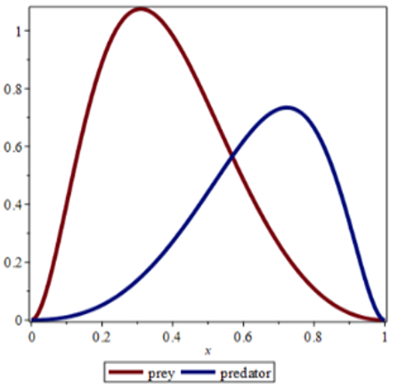
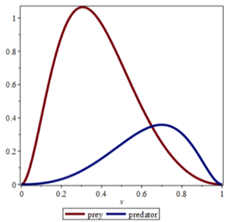
(a) SAGPM solution of $\emptyset(x, t)$ and $\varphi(x, t)$, at $t=0.5$
(b) SAGPM solution of $\emptyset(x, t)$ and $\varphi(x, t)$, at $t=1$
Figure 1. Solution of $\emptyset(x, t)$ and $\varphi(x, t)$, for (E1)
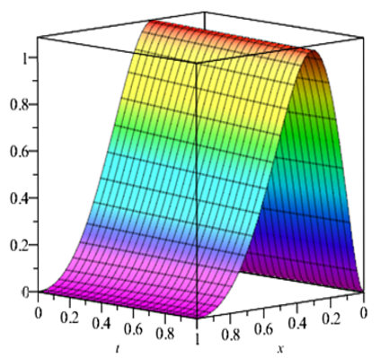
(a) SAGPM solution of $\emptyset(x, t)$
(b) SAGPM solution of φ(x, t)
Figure 2. Solution of $\emptyset(x, t)$ and $\varphi(x, t)$, for (E1)
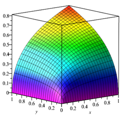
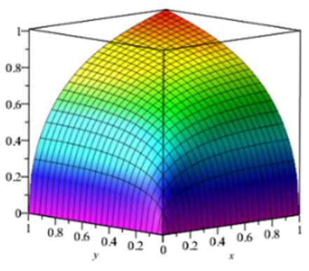
(a) SAGPM solution of $\varnothing(x, y, t)$
(b) SAGPM solution of $\varphi(x, y, t)$
Figure 3. SAGPM solution of $\emptyset(x, y, t)$, and $\varphi(x, y, t)$, for (E2), at $t=0.5$
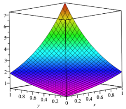
(a) SAGPM solution of $\varnothing(x, y, t)$
(b) SAGPM solution of $\varphi(x, y, t)$
Figure 4. SAGPM solution of $\emptyset(x, y, t)$, and $\varphi(x, y, t)$, for (E2), at $t=1$
In this part, we'll look at how the approximate analytical solutions from SAGPM for systems Eqs. (19) and (27) converge.
If we consider the system of equations in the following form:
$\begin{aligned} & \emptyset=F(\emptyset, \varphi) \\ & \varphi=G(\emptyset, \varphi)\end{aligned}$
where, F and G are non-linear operators. The solution of the present approach is equivalent to the following sequence:
$\begin{aligned} & S_n=\sum_{j=0}^n \emptyset_j=\sum_{j=0}^n a_j \frac{t^j}{(j) !} \\ & K_n=\sum_{j=0}^n \varphi_j=\sum_{j=0}^n b_j \frac{t^j}{(j) !}\end{aligned}$
Theorem (5.1): (Convergence of systems) [27]:
Let H be a Hilbert space, and let F, G be an operator from H into H, and $\emptyset$, φ be the exact solution of Eq. (35).
The approximate solutions:
$\begin{aligned} & \sum_{j=0}^{\infty} \emptyset_j=\sum_{j=0}^{\infty} a_j \frac{t^j}{(j) !} \\ & \sum_{j=0}^{\infty} \varphi_j=\sum_{j=0}^{\infty} b_j \frac{t^j}{(j) !}\end{aligned}$
are convergence to exact solutions $\emptyset, \varphi$ respectively when
$\begin{gathered}0 \leq C<1,\left\|\emptyset_{j+1}\right\| \leq C\left\|\emptyset_j\right\|, \forall i \in N \cup\{0\} \text { and } \exists 0 \leq \vartheta< \\ 1,\left\|\varphi_{j+1}\right\| \leq \vartheta\left\|\varphi_j\right\|, \forall j \in N \cup\{0\} .\end{gathered}$
Definition (5.2): For every $j \in N \cup\{0\}$, we define $C_j=\left\{\begin{array}{cc}\frac{\left\|\emptyset_{j+1}\right\|}{\left\|\emptyset_j\right\|}, & \left\|\emptyset_j\right\| \neq 0 \\ 0, & \text { otherwise }\end{array}\right.$ and $\vartheta_j=\left\{\begin{array}{c}\frac{\left\|\varphi_{j+1}\right\|}{\left\|\varphi_j\right\|}, \quad\left\|\varphi_j\right\| \neq 0 \\ 0, \quad \text { otherwise }\end{array}\right.$
Corollary (5.3): From the theorem above $\sum_{j=0}^{\infty} \emptyset_j=\sum_{j=0}^{\infty} a_j \frac{t^j}{(j) !}$ and $\sum_{j=0}^{\infty} \varphi_j=\sum_{j=0}^{\infty} b_j \frac{t^j}{(j) !}$ convergence to exact solutions $\varnothing$ and $\varphi$ when $0 \leq \mathrm{C}_j<$ 1 and $0 \leq \vartheta_j<1, j=0,1,2, \ldots$
Now, we apply the corollary as follows Table 5 to show how the analytical approximations in the two situations converge.
Table 5. The values of $C_j$ and $\vartheta_j$ using convergence condition at $0 \leq t \leq 1$, for $\emptyset(x, t)$ and $\varphi(x, t)$, in E1
|
Values of x |
$C_1$ |
$C_2$ |
ϑ1 |
ϑ2 |
|
0.3 |
0.7375526 |
0.6685518 |
0.7653308 |
0.4798963 |
|
0.6 |
0.7454224 |
0.5928046 |
0.7538936 |
0.4515959 |
|
0.9 |
0.7284150 |
0.7102612 |
0.7442563 |
0.4073371 |
The stability analysis of a particular model under investigation is a critical step in obtaining valid results and in determining the temporal and spatial step range in which the model is stable. This ensures that the model produces expected results in a time-efficient and accurate manner, rather than relying on trial and error. The stability analysis of predator-prey models is discussed in this section. Equilibrium points in nonlinear differential equations have a significant impact on model analysis. Balance points can be classified as node, saddle point, spiral or center based on the eigenvalues of the Jacobean matrix. Table 6 shows the fixed point ratings for systems Eqs. (19) and (27).
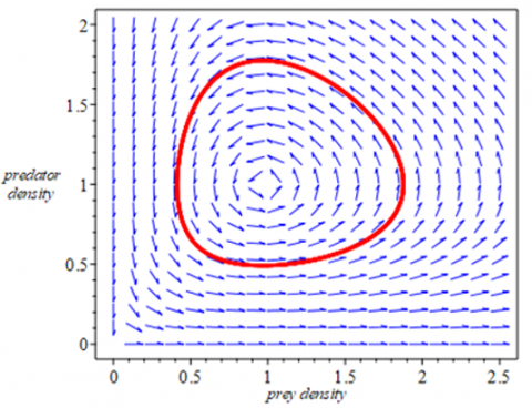
Where, α the serves as a representation of the fish, γ the death rate of the sharks, β and ε the interaction rate between fish and sharks. Figure 5 shows that there is little predation, which initially increases prey. After some time, more prey becomes available, which leads to an increase in the number of prey. As observed in the figure, this leads to a fall prey number. The system returns to its original configuration as prey abundance decreases and the number of prey begins to shrink again. Then the track starts looping. This will lead to the formation of an unstable vortex around the equilibrium points (1,0.96) and (0.98,0.58) for systems Eqs. (19) and (27), respectively.
Table 6. Classification of the equilibrium points for systems
|
Example |
Equilibrium Points |
Eigenvalues |
Stability |
|
1- |
(0,0) |
0.4, -0.29 |
Unstable |
|
(1,0.96) |
0.013+0.339i 0.013-0.339i |
||
|
2- |
(0,0) |
0.5, -0.3 |
Unstable |
|
(0.98,0.58) |
0.20+0.38i 0.20-0.38i |
(a) Local phase plane of systems (19), in the time interval [0, 50], with α=β=0.4, γ=0.29, ε=0.3, at the point x=0.4, when $\emptyset_0$ =0.9, φ0=0.4
(b) Local phase plane of system Eq. (27), in the time interval [0, 50], with α=0.5, β=ε=0.51, γ=0.3, at the points x=y=0.5, when $\emptyset_0$ =0.5, φ0=2.7
Figure 5. Local phase plane of systems
In this paper, a new method has been proposed and applied to solve the diffusive prey-predator systems. Two examples have been solved in one and two dimensions. The results obtained show that the new method is robust and efficient, with good convergence and high accuracy in terms of fewer errors and less CPU usage to solve distributed predator systems. Compared with other methods such as HPM, ADM and AGM, we can also conclude that the new method is an improvement of the standard approach AGM. In addition, approximate solutions were obtained with a small number of iterations for the serial solutions. Based on the results of this study, further research and development efforts can be directed towards applying the proposed method in other areas of computer science, engineering, and life sciences. Their use can be explored in analyzing social networks, understanding relationships and interactions between individuals, analyzing genetic data, and understanding the effects of genes on health and disease.
[1] Lotka, A.J., (1925). Elements of physical biology. Nature, 116: 461. https://doi.org/10.1038/116461b0
[2] Volterra, V., (1926). Fluctuations in the abundance of a species considered mathematically. Nature, 118: 55-560. https://doi.org/10.1038/118558a0
[3] Reeve, J.D., (1988). Environmental variability, migration, and persistence in host-parasitoid systems. The American Naturalist, 132(6): 810-836. https://doi.org/10.1086/284891
[4] Murdoch, W.W., Briggs, C.J., Nisbet R.M., Gurney W.S.C., Stewart-Oaten, A., (1992). Aggregation and stability in metapopulation models. The American Naturalist, 140(1): 41-58. https://doi.org/10.1086/285402
[5] Tiwari, V., Tripathi, J.P., Mishra, S., Upadhyay, R.K., (2020). Modeling the fear effect and stability of non-equilibrium patterns in mutually interfering predator-prey systems. Applied Mathematics and Computation, 371: 124948. https://doi.org/10.1016/j.amc.2019.124948
[6] Kekulthotuwage Don, S., Burrage, K., Helmstedt, K.J., Burrage, P.M. (2023). Stability switching in Lotka-Volterra and Ricker-type predator-prey systems with arbitrary step size. Axioms, 12(4): 390. https://doi.org/10.3390/axioms12040390
[7] Sun, Y.H., Chen, S.S., (2023). Stability and bifurcation in a reaction-diffusion-advection predator-prey model. Calculus of Variations and Partial Differential Equations 62(2): 61. https://doi.org/10.48550/arXiv.2212.04125
[8] Arif, M.S., Abodayeh, K., Ejaz, A. (2023). On the stability of the diffusive and non-diffusive predator-prey system with consuming resources and disease in prey species. Mathematical Biosciences and Engineering, 20(3): 5066-5093. https://doi.org/10.3934/mbe.2023235
[9] Chen, F.D. (2005). Positive periodic solutions of neutral Lotka-Volterra system with feedback control. Applied Mathematics and Computation, 162(3): 1279-1302. https://doi.org/10.1016/j.amc.2004.03.009
[10] Liu, Y.Q., Xin, B.G. (2011). Numerical solutions of a fractional predator-prey system. Advances in Difference Equations, 2011: 1-11. https://doi.org/10.1155/2011/190475
[11] Sabawi, Y.A., Pirdawood, M.A., Sadeeq, M.I. (2021). A compact fourth-order implicit-explicit Runge-Kutta type method for solving diffusive Lotka-Volterra system. Journal of Physics: Conference Series, 1999(1): 1-15. https://doi.org/10.1088/1742-6596/1999/1/012103
[12] Pal, D., Kesh, D., Mukherjee, D. (2023). Qualitative study of cross-diffusion and pattern formation in Leslie-Gower predator-prey model with fear and Allee effects. Chaos, Solitons & Fractals, 167: 113033. https://doi.org/10.1016/j.chaos.2022.113033
[13] Capone, F., Carfora, M.F., De Luca, R., Torcicollo, I. (2019). Turing patterns in a reaction-diffusion system modeling hunting cooperation. Mathematics and Computers in Simulation, 165: 172-180. https://doi.org/10.1016/j.matcom.2019.03.010
[14] Capone F., De Cataldis V., De Luca R., (2014). On the stability of a SEIR reaction diffusion model for infections under Neumann boundary conditions. Acta Applicandae Mathematicae, 132(1): 165-176. https://doi.org/10.1007/s10440-014-9899-7
[15] Capone, F., De Luca, R. (2017). On the nonlinear dynamics of an ecoepidemic reaction-diffusion model. International Journal of Non-Linear Mechanics, 95: 307-314. https://doi.org/10.1016/j.ijnonlinmec.2017.07.009
[16] Rionero, S. (2015). L 2-energy decay of convective nonlinear PDEs reaction-diffusion systems via auxiliary ODEs systems. Ricerche di Matematica, 64(2): 251-287. https://doi.org/10.1007/s11587-015-0231-2
[17] Rionero, S., Torcicollo, I. (2018). On the dynamics of a nonlinear reaction-diffusion duopoly model. International Journal of Non-Linear Mechanics, 99: 105-111. https://doi.org/10.1016/j.ijnonlinmec.2017.11.005
[18] Rionero, S., Torcicollo, I. (2014). Stability of a continuous reaction-diffusion Cournot-Kopel duopoly game model. Acta Applicandae Mathematicae, 132: 505-513.
[19] Torcicollo, I. (2013). On the dynamics of a non-linear Duopoly game model. International Journal of Non-Linear Mechanics, 57: 31-38. https://doi.org/10.1016/j.ijnonlinmec.2013.06.011
[20] Turing A.M., (1952). The chemical basis for morphogenesis. Philosophical Transactions of the Royal Society of London. Series B, Biological Sciences, 237, 641: 37-72. https://doi.org/10.1098/rstb.1952.0012
[21] Abdulameer, Y.A., Al-Saif, A.S.J.A. (2022). A well-founded analytical technique to solve 2d viscous flow between slowly expanding or contracting walls with weak permeability. Journal of Advanced Research in Fluid Mechanics and Thermal Sciences, 97(2): 39-56. https://doi.org/10.37934/arfmts.97.2.3956
[22] Hasan Z.A., Al-Saif A.S.J. (2022). A hybrid method with RDTM for solving the biological population model. Mathematical Theory and Modeling, 12(2): 1-11. https://doi.org/10.7176/MTM/12-2-01
[23] Al‐Griffi, T.A.J., Al‐Saif, A.S.J. (2022). Yang transform-homotopy perturbation method for solving a non‐Newtonian viscoelastic fluid flow on the turbine disk. ZAMM‐Journal of Applied Mathematics and Mechanics/Zeitschrift für Angewandte Mathematik und Mechanik, 102(8): e202100116. https://doi.org/10.1002/zamm.202100116
[24] Mirgolbabaee, H., Ledari, S.T., Ganji, D.D. (2017). Semi-analytical investigation on micropolar fluid flow and heat transfer in a permeable channel using AGM. Journal of the Association of Arab Universities for Basic and Applied Sciences, 24: 213-222. https://doi.org/10.1016/j.jaubas.2017.01.002
[25] Wu, B., Qian, Y. (2016). Padé approximation based on orthogonal polynomial. In 2016 International Conference on Modeling, Simulation and Optimization Technologies and Applications (MSOTA2016). Atlantis Press, pp. 249-252. https://doi.org/10.2991/msota-16.2016.54
[26] Maitama, S., Zhao, W. (2019). Maitama S., Zhao W.D., (2019). New integral transform: Shehu transform a generalization of Sumudu and Laplace transform for solving differential equations. International Journal of Analysis and Applications, 17(2): 167-190. http://doi.org/10.28924/2291-8639-17-2019-167
[27] Al-Jaberi A.K., Abdul-Wahab M.S., Buti R.H., (2022). A new approximate method for solving linear and non-linear differential equation systems. In AIP Conference Proceedings, Al-Samawah, Iraq, 2398(1): 1-17. http:/doi.org/10.1063/5.0094138