Abdurakhman![]()
© 2023 IIETA. This article is published by IIETA and is licensed under the CC BY 4.0 license (http://creativecommons.org/licenses/by/4.0/).
OPEN ACCESS
The Black-Scholes model, widely utilized for option pricing, has evolved into a trinomial model approach, providing an alternative means for determining option prices. Nonetheless, the trinomial model faces limitations in terms of time efficiency and accuracy. This study explores the acceleration of the trinomial option prices' convergence and computation time reduction using repeated Richardson extrapolation (RRE), achieved by recursively determining the order of incremental values. Comparative analysis with other extrapolation methods revealed that the RRE technique outperforms the Aitken Neville method by approximately 11%. Applied to a case study involving technology and energy stock option pricing, this technique minimized the required time steps to an average of 0.04 seconds, simultaneously achieving a mean square error (MSE) value of 0.835 compared to the Black-Scholes value. Consequently, the proposed methodology offers potential enhancements in computational efficiency for financial applications employing nested discrete-time models.
Richardson extrapolation, repeated Richardson extrapolation, trinomial model, European option, stocks
Option Pricing, a derivative financial asset, is intrinsically linked to the values of other assets or variables. A call option provides the purchaser with the privilege to acquire an asset at a predetermined price either on a designated date or any time prior to expiration. Conversely, a put option grants the buyer the right to sell the asset at an agreed price, and can be styled as either European or American [1].
The Black-Scholes option pricing model [2], along with its modifications by Merton [3], stands as a cornerstone of both option pricing theory and contemporary financial theory. This model presumes that stock prices follow a log-normal distribution and that transaction costs are absent. It calculates the fair price of a European call or put option, taking into account the current stock price, strike price, expiration time, risk-free interest rate, and volatility. The Black-Scholes-Merton (BSM) formula offers two significant benefits: it dispenses with the need for difficult or subjective parameter estimation, and its universal applicability and ease of use are well noted. The BSM formula is derived using arbitrage arguments, and incorporates the notions of risk-neutral probabilities and equivalent martingale measures, thereby enabling contingent asset pricing based on expected present value with parameters independent of risk aversion [4].
In addition to the BSM's explicit method, numerical methods such as binomial and trinomial models can also be employed for option pricing. In addition to the BSM explicit method, numerical methods such as binomial and trinomial models can also be used for option pricing. Numerical methods have been used in various fields, such as to improve optimization techniques [5], economics [6], anomalous diffusion [7], etc. It has been established by Josheski and Apostolov [8] that the trinomial model's convergence to BSM option pricing for European options is superior compared to its binomial counterpart. The binomial model [9] assumes that the underlying asset's price can either increase or decrease in each period and computes the probability of each outcome at each time step. The trinomial model [10, however, takes into consideration multiple factors affecting the option's price, such as the price of the underlying asset, the strike price of the option, the remaining time to expiration, and the volatility of the underlying asset.
The trinomial model, named for its three possible outcomes for the underlying asset's price at each time step - increase, decrease, or remain unchanged - estimates the option's value at each time step by computing the probability of each outcome, working backwards from the expiration date. A trinomial lattice is derived from the recombination of the trinomial tree's three branches [11]. The trinomial model is particularly useful for pre-training featured options, such as the American style option, and is often employed where the underlying asset's volatility is expected to change over time, as it allows for multiple possible outcomes at each time step.
Literature indicates that the trinomial model offers superior precision in determining option prices compared to the binomial model [12]. Furthermore, modifications to the trinomial tree model can expedite option pricing [13]. The theoretical convergence of the trinomial tree method, which ensures the reliability of option price calculations under regime switching, has been proven by Ma and Zhu [14]. The trinomial method demonstrates a convergence rate that is twice as fast as that of the Binomial and Black-Scholes methods [11]. Consequently, the development of the trinomial model is considered proficient in determining option prices. However, as a numerical method, the trinomial model is constrained by a slow convergence time. This research proposes an alternative solution to numerical methods for trinomial models using the repeated Richardson extrapolation (RRE) approach. This proposed alternative method is tested using various input parameters to generate option price data based on the trinomial model. Compared to the Cox, Ross, Rubinstein (CRR) binomial model, the trinomial model exhibits smoother convergence.
The remainder of this paper is organized as follows: Section 2 describes the RRE model for numerical solutions and compares it with other extrapolation methods. The development of the RRE algorithm on the trinomial model for option pricing is presented in Section 3, while Section 4 compares the computational results and convergence times of the various methods. Section 5 presents the implications for case studies in support of the theoretical results, and the final section concludes the paper.
Richardson extrapolation (RE) is a numerical analysis technique that corrects estimation errors by integrating several estimates linearly from different hyperparameter values without requiring detailed structural information [15]. In addition, RE is the most powerful numerical technique that can be used to improve the accuracy and performance of the underlying numerical method in solving large and complex problems [16]. Then, RE is a numerical method used to increase the accuracy of approximate solutions obtained through numerical integration or differentiation. The basic idea behind the RE technique is to use a sequence of approximations to a function, reducing the step size or mesh size, and then combining them in such a way that reduces errors. This is achieved by taking a linear combination of estimates that eliminates the low-order error term, resulting in a high-level estimate with better accuracy. The advantages of using RE techniques on numerical problems are increasing the accuracy and efficiency of the model, being able to predict errors, being applicable and easy to implement [17]. However, a limitation of this method is that it requires that the initial estimate converges with the true value of the function as the step size approaches zero. In addition, this method may be computationally expensive for large step sizes or high levels of approximation, so it is often used selectively in numerical algorithms where accuracy is required. This can be circumvented by repeating the RE method which is called repeated Richardson extrapolation (RRE). RRE involves applying RE several times to further increase the accuracy of the estimate [8]. Therefore, modification of the RRE model can be useful for improving the trinomial model of option pricing based on numerical patterns.
The general procedural concept related to RRE is as follows:
a. Approximating the unknown quantity
In the numerical analysis, the unknown quantity $\left(P_0\right)$ can be approximated with calculated quantity $(P(h))$ depending on parameter stepsize $h>0$ such that $\lim _{h \rightarrow 0} P(h)=P(0)=P_0$.
Under the assumption that $P(h)$ is sufficiently smooth function, we can write:
$P(h)=a_0+a_1 h^{\gamma_1}+\ldots+a_k h^{\gamma_k}+O\left(h^{\gamma_{k+1}}\right)$ (1)
where, $0<\gamma_1<\gamma_2<\ldots, a_1, a_2, \ldots$, unknown parameter and $h>0$. In particular, we have $a_0=P_0$.
b. Build the RRE model
According to Schmidt [18], the RRE can be built when we set $\gamma_j=\gamma j, j=1, \ldots, k$.
The idea of RE is to eliminate $h^{\gamma_1}$ from Eq. (1) so that we get a new approximation with higher order, say it $P_1(h)$ that has an error $P_1(h)-P(0)=O\left(h^{\gamma_2}\right), h \rightarrow 0^{+}$. Obviously $P_1(h)$ will be better approximation for $P(0)$ than $P(h)$ because of small $\mathrm{h}$ implied $h^{\gamma_2}<h^{\gamma_1}$. In the beginning, we compute $P(h)$ a number of times for successively smaller step sizes, $h_1>h_2>\ldots>0$, so that we obtain a sequence of approximation $P\left(h_1\right), P\left(h_2\right), \ldots$.
If we take step size $h_1=h$ to approximate $P(h)$, then Eq. (2) can be written:
$P\left(h_1\right)=a_0+\sum_{i=1}^k a_i h^{\gamma_i}+O\left(h^{\gamma_{k+1}}\right)$ (2)
We define $h_2=\omega h_1=\omega h$, where $\omega \in(0,1)$ such that satisfied $h_1>h_2>0$,
$P\left(h_2\right)=a_0+\sum_{i=1}^k a_i \omega^{\gamma_i} h^{\gamma_i}+O\left(h^{\gamma_{k+1}}\right)$ (3)
Multiplying Eq. (3) by $\omega^{\gamma_1}$,
$\omega^{\gamma_1} P\left(h_1\right)=\omega^{\gamma_1}\left(a_0+\sum_{i=1}^k a_i h^{\gamma_1}\right)+O\left(h^{\gamma_{k+1}}\right)$ (4)
Subtracting Eq. (3) by Eq. (4) gives,
$\frac{P\left(h_2\right)-\omega^{\gamma_1} P\left(h_1\right)}{\left(1-\omega^{\gamma_1}\right)}=a_0+\sum_{i=2}^k\left(\frac{\omega^{\gamma_i}-\omega^{\gamma_1}}{1-\omega^{\gamma_1}}\right) a_i h^{\gamma_i}+O\left(h^{\gamma_{k+1}}\right)$ (5)
Then we define:
$P\left(h_1, h_2\right)=\frac{P\left(h_2\right)-\omega^{\gamma_1 P\left(h_1\right)}}{\left(1-\omega^{\gamma_1}\right)}$ (6)
thus we get a new approximation for $a_0=P(0)$ such that,
$P\left(h_1, h_2\right)=a_0+\sum_{i=2}^k\left(\frac{\omega^{\gamma_i}-\omega^{\gamma_1}}{1-\omega^{\gamma_1}}\right) a_i h^{\gamma_i}+O\left(h^{\gamma_{k+1}}\right)$ (7)
Eq. (7) shows that $P\left(h_1, h_2\right)-P(0)=O\left(h^{\gamma_2}\right)$. The next step, we eliminate $h^{\gamma_2}$ using $P\left(h_1, h_2\right)$ and $P\left(h_2, h_3\right)$ and take $h_3=\omega h_2=\omega^2 h$ so that we get $P\left(h_1, h_2, h_3\right)-a_0=O\left(h^{\gamma_3}\right)$. We take the analogue process as the previous one to eliminate $h^{\gamma_3}, h^{\gamma_4}, \ldots$
RRE can be done by choosing a constant $\omega \in(0,1)$ and $h_0 \in(0, b)$, and let $h_i=h_0 \omega^i ; i=1,2, \ldots$ Obviously $\left\{h_i\right\}$ is a decreasing sequence in $(0, b)$, also $\lim _{i \rightarrow \infty} h_i=0$.
c. Recursive process for RRE
Define $P_0^{(j)}=P\left(h_j\right), j=0,1,2, \ldots, c_n=\omega^{\gamma_n}$ and calculate $P_n^{(j)}$ for $j=0,1,2, \ldots$ and $n=1,2, \ldots$ with recursive process:
$\begin{aligned} P_n^{(j)} & =\frac{P_{n-1}^{(j+1)}-c_n P_{n-1}^{(j)}}{1-c_n} =P_{n-1}^{(j+1)}+\frac{P_{n-1}^{(j+1)}-P_{n-1}^{(j)}}{\frac{1}{c_n}-1} .\end{aligned}$ (8)
Determining the value of $\gamma$, we use Taylor series $P(h)$ around $P(0)$ such that we have $\gamma=1$ and $\gamma_n=\gamma n=$ $\{1,2,3, \ldots, k\}$ for $n=1,2, \ldots, k$. After that, we can build extrapolation scheme:
$\begin{array}{ccc}T_{1,1} & & \\ T_{2,1} & T_{2,2} & \\ T_{3,1} & T_{3,2} & T_{3,3}\end{array}$
Recursive algorithm can be generalized using the triangle rule in extrapolation scheme:
Define $T_{i, 1}=P\left(h_i\right) ; i=1,2, \ldots \ldots$ For $i \geq 2$ and $j=$ $2,3, \ldots, i$ calculate:
$T_{i, j}=T_{i, j-1}+\frac{T_{i, j-1}-T_{i-1, j-1}}{\frac{h_{i-j+1}}{h_i}-1}$ (9)
Recursion (11) is special case of (10). This algorithm is known as Aitken-Neville algorithm. Let $\omega=\frac{1}{2}$, the recursive Eq. (11) become:
$T_{i, j}=T_{i, j-1}+\frac{T_{i, j-1}-T_{i-1, j-1}}{2^{j-1}-1} ; j=2,3, \ldots, i$ (10)
We take $h_0=H$, called $H$ as basic step. Because of $\omega=\frac{1}{2}$, we have sequence $h_i=\frac{H}{n_i} ; i=1,2, \ldots$, where $\left\{n_i\right\}=\left\{2^i\right\}=$ $\{2,4,8,16,32, \ldots\}$ as Romberg sequence.
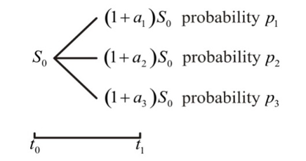
In trinomial model, stock price $S_0$ change by factors of $\rho_1$ which have three possibility values $\left(1+a_1\right),\left(1+a_2\right)$, $\left(1+a_3\right)$ with probabilities $p_1, p_2, p_3$ respectively and $p_1+$ $p_2+p_3=1$. The movement of stock price (see Figure 1) by one period of time is presented by following diagram:
Figure 1. The movement of stock price
As provided in reference [19], some parameters used in trinomial model are defined as follow:
$\begin{gathered}\left(1+a_1\right)=e^{\mu \Delta t+\sigma \sqrt{\left(\frac{3}{2}\right) \Delta t}}, \\ \left(1+a_2\right)=e^{\mu \Delta t}, \\ \left(1+a_3\right)=e^{\mu \Delta t-\sigma \sqrt{\left(\frac{3}{2}\right) \Delta t}}\end{gathered}$ (11)
And their probabilities are respectively
$p_j=\frac{r\left(3 a_j-\sum_{i=1}^3 a_i\right)+\sum_{i=1}^3 a_i^2-a_j \sum_{i=1}^3 a_i}{\sum_{i=1}^3 a_i^2-\left(\sum_{i=1}^3 a_i\right)^2} ; j=1,2,3$ (12)
where, the assumption of expected value of asset return is $\mu=\hat{r}, \hat{r}=e^{r \Delta t}-1$, and r is risk free rate. The use of those parameters in stock price movement leads to recombining trinomial tree. Trinomial model is a financial model used for pricing options. It is an extension of the Binomial model and allows for three possible outcomes at each step of the model. Here we try to implement RRE on the Trinomial option pricing model, we can follow these steps:
Overall, RRE can be a useful technique for improving the accuracy of the Trinomial model for pricing options. However, it is important to note that it can be computationally intensive, especially if multiple iterations are needed. Therefore, it is important to carefully balance the desired level of accuracy with the computational resources available. Here are procedures applying REE on trinomial model:
a. Establish the basic step and the number of repetitions. Basic step (H) is used to determine the sequence of approximation:
$\varphi\left(H ; h_1\right), \varphi\left(H ; h_2\right), \varphi\left(H ; h_3\right), \ldots$,
for step size $h_1>h_2>\ldots>0, h_i=\frac{H}{n_i}$, for $i=1,2, \ldots$. thereby $\left\{h_i\right\}$ is characterize using integers sequence $\left\{n_i\right\}$. In this case $\left\{n_i\right\}$ is Romberg sequence, $\mathfrak{F}_R:=\{2,4,8,16,32, \ldots\}$.
In trinomial model, basic step obtained from
$H=\frac{\tau}{N_0}$
where, τ is option’s remaining maturity, N0is the number of initial step.
b. Define the sequence of option price
Option values in the first column of extrapolation scheme are calculated using trinomial model.
c. Extrapolate the sequence
In this section, a numerical simulation of trinomial option pricing is performed. This simulation is carried out to calculate the speed of convergence and stability in predicting option prices. The stock price S=\$100, strike price K=\$100, remaining maturity of T=6 months, set volatility={0.2,0.3,0.4,0.5,0.6,0.7,0.8}, and the risk-free rate is 5%. The simulation uses R software by designing a function algorithm for the trinomial model using Richardson (RRE) and Neville-Aitken (RNA). The simulation results are compared with the option prices of the Black-Scholes (B-S) model. Then, below is a table showing the results of the call option valuation.
Table 1. Time comparison
|
Volatility |
B-S Option Price (OP) |
RNA |
RRE |
||
|
OP |
Time(s) |
OP |
Time(s) |
||
|
0.2 |
6.889 |
6.984 |
0.051 |
6.966 |
0.121 |
|
0.3 |
9.635 |
9.815 |
0.044 |
9.860 |
0.051 |
|
0.4 |
12.385 |
12.896 |
0.032 |
12.914 |
0.036 |
|
0.5 |
15.127 |
16.167 |
0.034 |
16.122 |
0.027 |
|
0.6 |
17.855 |
19.634 |
0.025 |
19.506 |
0.023 |
|
0.7 |
20.564 |
23.336 |
0.033 |
23.105 |
0.026 |
|
0.8 |
23.251 |
27.317 |
0.031 |
27.132 |
0.027 |
Regarding the RRE model, it provides relatively fast computational value compared to RNA (see Table 1). In addition, the option price given the RE-based trinomial model is closer to the B-S value than RNA with an average convergence time of 0.04 and outperforming NA by 11% against the B-S option price. However, in simulations with low volatility, RNA is superior based on estimated option prices and time velocity. It can be assumed that if prices for small asset price fluctuations can use trinomial models based on RNA, while for cases with high levels of volatility can use RRE. In conclusion, this proves that the RRE method is more efficient in calculating option prices.
Option pricing tests were performed for stock option price analysis. Then, we have collected data that is divided into two categories, namely the technology and energy sectors. The technology sector consists of Google (GOOGL), Apple (AAPL), Tesla (TSLA), and Amazone Inc (AMZN) daily stock data. Meanwhile, the daily stock prices for Exxon Mobil Corp (XOM), Shell PLC (SHEL), Occidental Petroleum Corp (OXY), and Marathon Oil Corp (MRO) are for the energy sector. Daily stock data was taken from April 2021 to April 2023 from the Yahoo Finance website using Software R. The options prices compared are call options. We use the United States Bank Daily Treasury Bill Rate, which is 0.05. This study calculates call options on government shares. The steps are as follows: (1) descriptive analysis related to stocks; (2) calculating returns using a compound log return; (3) Calculate the call option using the RRE in Eq. (10); (4) Calculate the call option using B-S; (5) Compare the results of each model.
5.1 Descriptive statistics of stock prices
a. Technology Sector
Figure 2 shows the time series plot of each stock: GOOGL, AAPL, AMZN, TSLA. Google is a multinational technology company that specializes in Internet-related services and products, including online advertising technologies, search engines, cloud computing, software, and hardware. Google was founded in 1998 by Larry Page and Sergey Brin while they were Ph.D. students at Stanford University, and it has since become one of the world's most valuable companies, with a market capitalization of over \$1 trillion as of 2021. Apple is a multinational technology company based in California, that designs, develops, and sells consumer electronics, computer software, and online services. The company was founded in 1976 by Steve Jobs, Steve Wozniak, and Ronald Wayne, and it is now one of the world's most valuable companies with a market capitalization of over \$2 trillion as of 2021. Tesla, Inc. is a US-based company that specializes in the design, development, and production of electric vehicles, energy storage systems, and solar products. The company was founded in 2003 by Elon Musk and friends, and it is headquartered in Palo Alto, California. Tesla is one of the world's most valuable car companies, with a market capitalization of over \$700 billion as of 2021. Amazon is a multinational technology company based in Seattle, Washington, that focuses on e-commerce, cloud computing, digital streaming, and artificial intelligence. The company was founded in 1994 by Jeff Bezos. Today, Amazon is one of the world's largest online retailers, selling a wide range of products and services, including books, electronics, clothing, groceries, and more. As of 2021, Amazon is one of the most valuable companies in the world, with a market capitalization of over \$1.6 trillion.
Figure 2. Plot time series of tech stock price movements
Table 2 shows a descriptive statistical comparison of closing prices and daily stock returns in the technology sector. Then based on these statistics it is known that for two years the skewness value of each share is close to zero, while the kurtosis value is at odds with a value of 3 (this value if the kurtosis is said to be normal). In addition, the range between the minimum and maximum values is relatively wide. Thus, the volatility of these stocks is relatively high, based on the computational comparison part, the RRE model will be easy to adapt.
Regarding descriptive statistics on stock returns for the technology sector, they are presented in Table 2. There are two stocks that have negative average returns, namely AMZN and TSLA, while the other two stocks have positive returns, although small. In addition, as with the closing price, stock returns also have a skewness value close to zero and a kurtosis value of less than 3, only AMZN has a kurtosis value of more than 3.
Table 2. Descriptive statistics technology sector
|
Closing Price |
||||
|
Descriptive Statistics |
Closing Price |
|||
|
GOOGL |
AAPL |
TSLA |
AMZN |
|
|
Mean |
118.949 |
151.193 |
250.632 |
137.271 |
|
SD |
18.382 |
13.725 |
63.869 |
31.402 |
|
Median |
117.597 |
149.640 |
239.707 |
142.570 |
|
Min |
83.430 |
122.770 |
108.100 |
81.820 |
|
Max |
149.838 |
182.010 |
409.970 |
186.570 |
|
Skew |
-0.024 |
0.100 |
0.235 |
-0.180 |
|
Kurtosis |
-1.261 |
-0.652 |
-0.468 |
-1.507 |
|
Return |
||||
|
Descriptive Statistics |
Return |
|||
|
GOOGL |
AAPL |
TSLA |
AMZN |
|
|
Mean |
0.00005 |
0.00061 |
-0.00004 |
-0.00056 |
|
SD |
0.02096 |
0.01878 |
0.03820 |
0.02568 |
|
Median |
0.00022 |
0.00050 |
0.00126 |
-0.00046 |
|
Min |
-0.09141 |
-0.05868 |
-0.12242 |
-0.14049 |
|
Max |
0.07656 |
0.08897 |
0.13532 |
0.13536 |
|
Skew |
0.07778 |
0.13439 |
-0.06845 |
0.09696 |
|
Kurtosis |
1.72455 |
1.52580 |
0.98736 |
4.49422 |
Figure 3. Plot time series of energy stock price movements
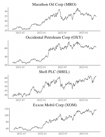
b. Energy Sector
XOM (Exxon Mobil), is an American multinational oil and gas corporation that operates in more than 200 countries. It is one of the largest publicly traded companies in the world and is listed on the NYSE. OXY (Occidental Petroleum Corporation) is another American multinational petroleum and natural gas exploration and production company. It is also listed on the NYSE and operates in countries such as the United States, Colombia, and Qatar. MRO (Marathon Oil Corporation) is an American oil and gas exploration and production company that is listed on the NYSE. MRO operates in countries such as the United States, Equatorial Guinea, and Libya. SHEL (Royal Dutch Shell) is a British-Dutch multinational oil and gas company that is listed on the London, Amsterdam, and New York stock exchanges. SHEL operates in more than 70 countries and is one of the largest oil companies in the world. The time series plot for Energy sector could be seen in Figure 3.
Table 3. Descriptive statistics energy sector
|
Closing Price |
||||
|
Descriptive Statistics |
Closing Price |
|||
|
MRO |
OXY |
SHEL |
XOM |
|
|
Mean |
21.219 |
49.137 |
50.404 |
83.593 |
|
SD |
6.298 |
17.095 |
7.145 |
20.482 |
|
Median |
22.670 |
57.870 |
52.020 |
85.050 |
|
Min |
10.670 |
21.950 |
37.080 |
52.730 |
|
Max |
33.030 |
75.970 |
62.580 |
119.170 |
|
Skew |
-0.214 |
-0.224 |
-0.243 |
0.078 |
|
Kurtosis |
-1.256 |
-1.653 |
-1.217 |
-1.418 |
|
Return |
||||
|
Descriptive Statistics |
Return |
|||
|
MRO |
OXY |
SHEL |
XOM |
|
|
Mean |
0.00216 |
0.00237 |
0.00128 |
0.00184 |
|
SD |
0.03132 |
0.03229 |
0.01954 |
0.01989 |
|
Median |
0.00151 |
-0.00071 |
0.00066 |
0.00228 |
|
Min |
-0.14032 |
-0.10933 |
-0.08082 |
-0.07885 |
|
Max |
0.13625 |
0.17592 |
0.05505 |
0.06411 |
|
Skew |
0.05907 |
0.51957 |
-0.21687 |
-0.16301 |
|
Kurtosis |
1.45229 |
2.08790 |
1.13311 |
0.67998 |
Table 3 shows a descriptive statistical comparison of closing prices and daily stock returns in the energy sector. The average price for the energy sector is relatively lower than that for the technology sector. However, it has a relatively large average (see Table 3). Then, it is known that for two years the skewness value of each stock is close to zero, while the kurtosis value is less than 3. In addition, the range between the minimum and maximum values is relatively wide. Thus, the volatility of these stocks is relatively high. For stock returns, the average stock value is still positive, this indicates that investment in this sector has a low level of risk. In addition, as with the closing price, stock returns also have a skewness value close to zero and a kurtosis value of less than 3
5.2 Option pricing comparisons
The results of a comparison of estimated option prices using the trinomial approach based on RRE in case studies of technology and energy stocks are presented in Table 4. The Trinomial RRE method works well and can produce option prices that are very close to the prices produced by the Black-Scholes model. The average difference in market prices with the RRE and BS models is 2.819 and 1.979, respectively. Meanwhile, the difference in the value of the RRE model with the BS is 0.835. In addition, the RRE method is very effective in reducing the computational costs of option pricing, as it allows the use of coarser grids while maintaining high accuracy. Therefore, the Trinomial RRE method is a valuable tool for traders and investors who wish to value call options accurately and efficiently.
Table 4. Call option price estimation
|
Stock |
S0 |
K |
RRE |
BS |
Market Price |
|
GOOGL |
105.97 |
100 |
6.913 |
7.879 |
14.05 |
|
AAPL |
165.33 |
115 |
51.487 |
52.860 |
53.34 |
|
AMZN |
106.96 |
100 |
8.458 |
9.429 |
15.55 |
|
TSLA |
162.99 |
80 |
85.909 |
87.055 |
86.95 |
|
MRO |
24.73 |
15 |
9.271 |
9.460 |
11.5 |
|
OXY |
62.76 |
55 |
7.678 |
8.228 |
10.8 |
|
XOM |
115.64 |
85 |
32.128 |
33.109 |
31.05 |
|
SHEL |
61.65 |
55 |
7.263 |
7.818 |
8.42 |
The result of this experiment is that the RRE technique can be applied to the Trinomial option pricing model. This technique accelerates the rate of trinomial convergence with the result that it approaches the value of the option price using the Black-Scholes method, which is still used to determine the price of options in financial markets. This extrapolation technique allows for a reduced number of steps required and faster computation times. Overall, this paper presents a promising approach to option pricing in the trinomial model, which may be applicable in a variety of financial situations. However, like all financial models, the trinomial model has limitations and assumptions that may not always hold true under real-world market conditions. It is important to use multiple models and consider various factors when assessing options or making investment decisions. For further research, you can use the RRE method on other financial models to determine.
I would like to express my sincere appreciation to the following individuals and organizations who have made this research project possible. I would like to thank the UGM for providing the necessary resources, facilities, and funding to carry out this research project. Lastly, I am indebted to my family and friends for their unwavering support, encouragement, and understanding throughout this journey. Thank you all for your contributions and support. The authors would like to thank the anonymous referee experts for their appropriate and constructive suggestions to improve this research paper.
[1] de Andrés-Sánchez, J. (2023). A systematic review of the interactions of fuzzy set theory and option pricing. Expert Systems with Applications, 223: 119868. https://doi.org/10.1016/j.eswa.2023.119868
[2] Black, F., Scholes, M. (1973). The pricing of options and corporate liabilities. Journal of Political Economy, 81(3): 637-654.
[3] Merton, R.C. (1998). Applications of option-pricing theory: Twenty-five years later. The American Economic Review, 88(3): 323-349.
[4] Broadie, M., Detemple, J.B. (2004). Anniversary article: Option pricing: Valuation models and applications. Management Science, 50(9): 1145-1177. https://doi.org/10.1287/mnsc.1040.0275
[5] Semchedine, M., Bensoula, N. (2022). Enhanced black widow algorithm for numerical functions optimization. Revue d'Intelligence Artificielle, 36(1): 1-11. https://doi.org/10.18280/ria.360101
[6] Mutegi, M.A., Nnamdi, N. (2021). Filter feeding allogenic engineering optimization algorithm for economic dispatch. International Journal of Energy Production and Management, 6(2): 113-128. https://doi.org/10.2495/EQ-V6-N2-113-128
[7] Tang, Z.C., Fu, Z.J. (2021). Generalized finite difference method for anomalous diffusion on surfaces. International Journal of Computational Methods and Experimental Measurements, 9(1): 63-73. https://doi.org/10.2495/CMEM-V9-N1-63-73
[8] Josheski, D., Apostolov, M. (2020). A review of the binomial and trinomial models for option pricing and their convergence to the Black-Scholes model determined option prices. Econometrics Ekonometria Advances in Applied Data Analysis, 24(2): 53-85. https://doi.org/10.15611/eada.2020.2.05
[9] Breen, R. (1991). The accelerated binomial option pricing model. Journal of Financial and Quantitative Analysis, 26(2): 153-164. https://doi.org/10.2307/2331262
[10] Kamrad, B., Ritchken, P. (1991). Multinomial approximating models for options with k state variables. Management Science, 37(12): 1640-1652. https://doi.org/10.1287/mnsc.37.12.1640
[11] Langat, K.K., Mwaniki, J.I., Kiprop, G.K. (2019). Pricing options using trinomial lattice method. Journal of Finance and Economics, 7(3): 81-87. https://doi.org/10.12691/jfe-7-3-1
[12] Dou, C. (2017). The equation of real option value under trinomial tree model. Open Journal of Social Sciences, 5(3): 74646. https://doi.org/10.4236/jss.2017.53001
[13] Yuen, F.L., Yang, H. (2010). Option pricing with regime switching by trinomial tree method. Journal of Computational and Applied Mathematics, 233(8): 1821-1833. https://doi.org/10.1016/j.cam.2009.09.019
[14] Ma, J., Zhu, T. (2015). Convergence rates of trinomial tree methods for option pricing under regime-switching models. Applied Mathematics Letters, 39: 13-18. https://doi.org/10.1016/j.aml.2014.07.020
[15] Bach, F. (2021). On the effectiveness of Richardson extrapolation in data science. SIAM Journal on Mathematics of Data Science, 3(4): 1251-1277. https://doi.org/10.1137/21M1397349
[16] Bayleyegn, T., Havasi, Á. (2021). The method of multiple Richardson extrapolation. Developments in Computer Science.
[17] Bayleyegn, T., Havasi, Á. (2021). Multiple Richardson extrapolation applied to explicit Runge–Kutta methods. In: Dimov, I., Fidanova, S. (eds) Advances in High Performance Computing. HPC 2019. Studies in Computational Intelligence, vol. 902. Springer, Cham. https://doi.org/10.1007/978-3-030-55347-0_22
[18] Sidi, A. (2003). Practical Extrapolation Methods. Cambridge University Press.
[19] Abdurakhman, Subanar, Guritno, S., Zoejoeti, Z. (2006). Valuing trinomial option pricing with pseudoinverse matrix. Journal of the Indonesian Mathematical Society, 12(2): 131-140.