Youssef Mhanni*![]() | Youssef Lagmich
| Youssef Lagmich![]()
© 2023 IIETA. This article is published by IIETA and is licensed under the CC BY 4.0 license (http://creativecommons.org/licenses/by/4.0/).
OPEN ACCESS
This study presents a novel algorithm designed to facilitate intelligent navigation and obstacle avoidance for mobile robots. The proposed algorithm provides a reliable means for robots to navigate complex environments, skillfully negotiating both static and dynamic obstacles while identifying the most efficient path from a start point to a destination. The principal aim is to guide a robot's traversal through various environments, preventing collision with obstacles while ensuring an optimal path is followed. The robot's trajectories are generated using an optimized version of the artificial potential field (APF) technique, renowned for its simplicity and effectiveness in dynamic and intricate environments. The developed algorithm calculates both attraction and repulsion forces between the robot and various elements within its environment, including the goal, obstacles, and other robots. This holistic approach ensures the efficiency and continuity of the plotted trajectory. To further refine the robot's movement towards the goal, a fuzzy logic-based intelligent controller is incorporated. The integration of fuzzy logic control (FLC) with the APF technique allows the system to strategically plan the robot's path. This is achieved by determining the subsequent location point and calculating the required angular and linear velocities using a forward linkage controller (FLC). The efficacy of the approach is validated through a series of real-time experiments and simulations. The refined algorithm, with appropriately tuned parameters, is implemented within the Robotics Operating System (ROS) environment using the Gazebo simulator. The results obtained provide a comprehensive evaluation of the modified potential field technique's applicability, validity, and optimal performance in task completion scenarios. Through the integration of the optimized artificial potential field and fuzzy logic control, the proposed approach presents a robust solution for the safe and efficient navigation of mobile robots in complex environments.
robot navigation, artificial potential field, fuzzy logic control, intelligent controller, robotics operating system (ROS), obstacle avoidance, gazebo simulator robot
The quest for autonomy is driving rapid advancements in numerous sectors, with one prominent area of focus being robotics, specifically in the domains of obstacle avoidance and autonomous path planning for mobile robots. The critical challenge lies in devising efficient routes for such autonomous entities, enabling secure traversal from one point to another while minimizing the journey duration and distance [1]. The goal is to equip robots with the capability to automatically determine and execute a sequence of safe, collision-free maneuvers, thereby ensuring task completion within their operational environments.
Path planning strategies can be broadly classified into two categories: global route planning, predicated on pre-existing environmental data, and local route planning, adapting dynamically to real-time sensor data [2]. Central to robot navigation, obstacle avoidance algorithms empower robots to navigate their surroundings without colliding with objects in their path or while pursuing a designated goal [3]. Combined with the robot's current position and a map of the navigable area, these algorithms facilitate path planning techniques to ascertain and implement the optimal course of action, thereby minimizing collision risks.
This research primarily aims to develop strategies for modulating robot movement to effectively circumvent collisions. However, the algorithms derived from these strategies invariably confront two significant challenges: a lack of scalability due to high computational demands and an inability to assure the desired system performance.
The Artificial Potential Field (APF) method, first proposed by Khatib in 1985 [4], is a widely adopted strategy for mobile robot path planning. This approach entails constructing a potential field within the robot's operational environment, acting as an attractor towards the target and a repellant for obstacles [5-7]. The environment is modeled as a potential field, with the goal serving as a potential well and obstacles as potential hills. The potential field is further manipulated by assigning a negative value to the goal and a positive value to the obstacles, subjecting the mobile robot to an artificial potential force.
Recognizing that background algorithms for obstacle avoidance vary considerably, each proposing unique and innovative strategies for collision avoidance, is crucial [8, 9]. A substantial objective of this study is to explore the potential of integrating low-cost sensors and high-quality bathymetry with historical navigation methodologies in autonomous underwater vehicle (AUV) localization and navigation algorithms [10].
Obstacle avoidance can also be facilitated through the deployment of fuzzy logic and neuro-fuzzy networks [11, 12]. Fuzzy logic control systems have become indispensable tools in mobile robot navigation and motion control, facilitating their adaptation to changing environments [13, 14]. The application of fuzzy logic theory to the speed-and-depth control of AUVs has been examined, highlighting the influence of AUV motion on navigation depth and pitch [15, 16]. This suggests the potential for mobile robots to autonomously navigate a space, leveraging the recommended controller without human intervention.
The primary objective of this research is to devise an efficient, user-friendly algorithm for path planning by integrating the APF method with a Fuzzy Logic technique. This combined approach is posited to be effective in both static environments and in the presence of static obstacles. By enhancing the APF method and applying Newton's Second Law, the APF is optimized to yield optimal path planning and Fuzzy Logic Control (FLC) for effective movement of the robot towards the target.
Key research questions include:
How can the APF method be enhanced to improve path planning in complex and dynamic environments?
What is the impact of integrating Fuzzy Logic Control with the APF method on collision avoidance and trajectory efficiency?
Can the proposed combined approach deliver scalable and reliable performance for robot navigation across various environments?
The potential benefits of self-adaptive recurrent neuro-fuzzy control for AUVs will also be investigated through simulation results [17], demonstrating the ability to guide AUVs despite environmental forces and enabling them to proceed in their preferred directions.
The remainder of this paper is organized as follows: Section 1 provides both graphical and mathematical representations of the APF, along with a discussion on the global challenge of robot collisions with barriers. Section 2 provides mathematical formulations and analyses of the robot's dynamics and kinematics. Section 3 presents the graphical representation of the APF FLC and the parameters used in this study. Section 4 presents the simulation results, including details of the Robotics Operating System (ROS) [18, 19]. Finally, Section 5 concludes the paper, offering recommendations for future research avenues.
2.1 Problem description
In autonomous robot navigation, moving from one location to another in the absence of obstacles is a straightforward task. However, even a single obstacle in the robot's path can lead to a significant challenge. The presence of obstacles obstructs the robot's progress, rendering it incapable of completing its task successfully. Instead, it may collide with the obstacle, resulting in damage to both the robot itself and its navigation guidance, as illustrated in the figure below. This obstacle avoidance problem is critical to address to ensure safe and efficient robot movement in complex and dynamic environments.
(a)
(b)
Figure 1. A scenario in which a mobile robot doesn't use any avoidance algorithm
The primary objective of this research is to design an advanced path planning algorithm capable of efficiently finding the shortest and obstacle-free route to the goal point in complex environments. To achieve this, we employ a fuzzy logic controller to determine the robot's trajectory during its autonomous navigation. As depicted in Figure 1, we observe the robot encountering an obstacle, hindering its progress towards the goal. Currently, there is a lack of suitable algorithms to effectively avoid obstacles in the path planning process. In this study, we propose a method that utilizes an enhanced artificial potential field to identify the desired position and optimal orientation at each subsequent point along the path. Through this approach, we aim to enhance obstacle avoidance capabilities and ensure successful completion of tasks for autonomous mobile robots
2.2 Artificial potential field process
The challenge of preventing collisions between a robot and obstacles in a planar environment is depicted in Figure 1. To address this challenge, the artificial potential field model is utilized, guiding the robot with attractive forces towards its goal while repulsive forces steer it away from obstacles. The model provides multiple alternative paths for the robot to navigate around obstacles, ensuring efficient and collision-free movement. By dynamically adjusting forces based on real-time conditions, the artificial potential field model empowers the robot to reach its destination without delays or collisions
Figure 2. Representation of an artificial potential field with a potential target
In a two-dimensional space, the robot faces the challenge of avoiding collisions with the obstruction depicted in Figure 2. The artificial potential field model guides the robot with attractive forces towards its destination while repulsive forces prevent collisions with the obstacle. The model ensures that the robot safely navigates around the obstruction, reaching its goal without any collisions in the two-dimensional environment [4].
$U_{\text {Total }}(q)=U_{\text {att }}(q)+U_{\text {rep }}(q)$ (1)
$q$ denotes the number of degrees of freedom. $U_{\text {Total }}(q), U_{\text {att }}(q)$ and $U_{\text {rep }}(q)$ are shorthand as the abbreviations for the artificial potential field, attraction potential energy, and repulsion potential energy, respectively.
This research focuses on simulating a mobile robot's motion in a two-dimensional $(x, y)$ space. The study aims to develop a new representation of the equation governing the robot's movement to enhance path planning and obstacle avoidance capabilities. By leveraging this novel equation, the research seeks to improve the efficiency and intelligence of the robot's navigation towards its destination in two-dimensional environments. The ultimate goal is to contribute valuable insights to the field of mobile robotics and advance autonomous navigation capabilities in two-dimensional spaces.
$U_{\text {Total }}(x, y)=U_{\text {att }}(x, y)+U_{\text {rep }}(x, y)$ (2)
If so, we may express the gradient function as:
$F_{n e t}(x, y)=F_{a t t}(x, y)+F_{r e p}(x, y)$ (3)
with
$F_{a t t}=-\nabla\left[\left(U_{a t t}(x, y)\right)\right]$ (4)
$F_{r e p}=-\nabla\left[\left(U_{r e p}(x, y)\right)\right]$ (5)
As, $F_{\text {att }}$ represents the attractive force that propels the mobile robot to its destination and represents the repulsive force that is generated $y, U_{\text {rep }}(x, y)$. The value indicates how far away the mobile robot is from its intended destination. The attractive potential field, $U_{a t t}(x, y)$. is therefore simply expressed as where $(x, y)$.
The robot's current position may be represented by the coordinates representing the present $\left(x_{r o b}, y_{r o b}\right)$. Even before it made an effort to get to the destination spot, the robot was already being pulled in that direction by the attractive force. Therefore, the attraction typically returns to zero as the robot gets closer to the target point. The enticingly promising field $U_{\text {att }}(x, y)$ of possibility in Dimension.
$U_{\text {att }}=\frac{1}{2} k_{\text {att }} \ell_{\text {goal }}^2$ (6)
With $K_{\text {att }}$ is the attractive potential field gain and $l_{\text {goal }}$ the distance between the robot and the point of destination, and write it using this formula.
$l_{\text {goal }}\left(X_{\text {goal }}, X_{\text {rob }}\right)=\left\|X_{\text {rob }}-X_{\text {goal }}\right\|$ (7)
and
$l_{\text {goal }}=\sqrt{\left(x_{\text {rob }}-x_{\text {gaol }}\right)^2+\left(y_{\text {rob }}-y_{\text {goal }}\right)^2}$ (8)
and we get
$U_{\text {att }}=\frac{1}{2} k_{a t t}\left(\left(x_{\text {rob }}-x_{\text {gaol }}\right)^2+\left(y_{\text {rob }}-y_{\text {goal }}\right)^2\right)$ (9)
The value of $F_{\text {att }}$ indicates how far away the mobile robot is from its intended destination. The attractive potential field $U_{a t t}(X)$ is therefore simply expressed as where $x$ is the attractive potential and $K_p$ is the gain factor of attraction.
$U_{\text {rep }}=\left\{\begin{array}{cc}\frac{1}{2} k_{\text {rep }}\left(\frac{1}{d_{o b s}}-\frac{1}{q^*}\right)^2, & d_{o b s}<q^* \\ 0 & \text { otherwise }\end{array}\right.$ (10)
where, $x$ is the location of the robot as represented by $\left(\mathrm{x}_{r o b}, \mathrm{y}_{r o b}\right), x_{o b s}$ is the position of the obstacles as represented by $\left(\mathrm{x}_{o b s l}, \mathrm{y}_{\text {obsl }}\right)$, and $\mathrm{x}_{\text {goal }}$ is the position of the objective as represented by $\left(\mathrm{x}_{\text {goal }}, \mathrm{y}_{\text {goal }}\right)$.
$d_{o b s}\left(X, X_{\text {goal }}\right)=\left\|X_{o b s l}-X\right\|$ (11)
So
$\begin{aligned} & d_{o b s}\left(X, X_{o b s}\right)= \\ & \sqrt{\left(x_{\text {rob }}-x_{o b s l}\right)^2+\left(y_{\text {rob }}-y_{o b s l}\right)^2}\end{aligned}$ (12)
In Eq. (12), the representation captures the shortest path in two-dimensional space between the robot and the target. Subsequently, the functions of attraction and repulsion are expressed as follows:
$F_{a t t}=-\nabla\left(U_{a t t}(x, y)\right)$ (13)
Since we have two different variables, we can calculate $x$ and $y$ to get the two different forces.
$\begin{gathered}\nabla U_{\text {att }}(q)=\nabla\left(\frac{1}{2} k_{\text {att }} l_{\text {goal }}^2\left(q, q_{\text {goal }}\right)\right), \\ =\frac{1}{2} k_{\text {att }} \nabla l_{\text {goal }}^2\left(q, q_{\text {goal }}\right),=k_{\text {att }}\left(q-q_{\text {goal }}\right),\end{gathered}$ (14)
So, the attractive forces, $F_{x a t t}$.and $F_{y a t t}$, defined by the following $x, y$ are as follows:
$\left\{\begin{array}{l}F_{x a t t}=-\frac{\partial U_{a t t}(x, y)}{\partial x}=-k_{\text {att }}\left(x_{\text {rob }}-x_{\text {goal }}\right) \\ F_{\text {yatt }}=-\frac{\partial U_{a t t}(x, y)}{\partial y}=-k_{\text {att }}\left(y_{\text {rob }}-y_{\text {goal }}\right)\end{array}\right.$ (15)
As a consequence of this, we can conclude that the overall attractive force is equivalent to the aggregate of the attractive forces. As a consequence of this, we can conclude that the overall attractive force is equivalent to the aggregate of the attractive forces. $F_{x a t t}$ and $F_{y a t t}$ :
$F_{x n e t}=F_{x a t t}+F_{x r e p}$ (16)
the repulsive potential field, denoted by the symbol $U_{\text {rep }}$, that is generated as a result of the proximity of the Robot to the obstructions: the repulsive potential field, denoted by the symbol $U_{\text {rep }}$, that is produced as a result of the relative distance between the robot and the obstacles is as follows:
$U_{r e p_i}(q)=\left\{\begin{array}{cl}\frac{1}{2} k_{r e p}\left(\frac{1}{d_{o b s}(q)}-\frac{1}{Q^*}\right)^2, & d_{o b s}<Q^* \\ 0 & \text { otherwise }\end{array}\right.$ (17)
where, $i$ is the current obstacle's order number
With:
$d_{o b s}\left(X_{\text {rob }}, X_{\text {obsl }}\right)=\left\|X_{o b s l}-X_{\text {rob }}\right\|$ (18)
So
$d_{o b s}\left(X, X_{o b s}\right)=\sqrt{\left(x_{r o b}-x_{o b s l}\right)^2+\left(y_{r o b}-y_{o b s l}\right)^2}$ (19)
When there are $n$ number of obstructions, the total repulsive function is:
$U_{r e p}(q)=\sum_{i=1}^n U_{r e p_i}(q)$ (20)
Whereas, in our research, we focused on a single obstacle so that we could acquire it.
$U_{r e p}(q)=U_{r e p_i}(q)$ (21)
Whose gradient is:
$\nabla U_{r e p}(q)=\left\{\begin{array}{cc}k_{r e p}\left(\frac{1}{Q^*}-\frac{1}{d_{o b s}(q)}\right) \frac{1}{d_{o b s}^2(q)} \nabla d_{o b s}(q), & d_{o b s}(q)<Q^* \\ 0 & \text { otherwise }\end{array}\right.$ (22)
A repulsive force is defined as a negative gradient of the repulsive potential, $U_{\text {rep }}(x, y)$ :
$F_{r e p}=-\nabla\left(U_{r e p}(x, y)\right)$ (23)
The definition of the attracting forces, indicated by, that follow $y$ and $x$ is as follows:
$\left\{\begin{array}{l}F_{x r e p}=-\frac{\partial U_{r e p}(x, y)}{\partial x} \\ F_{y r e p}=-\frac{\partial U_{r e p}(x, y)}{\partial y}\end{array}\right.$ (24)
$x$ following attractive forces are defined:
$F_{x r e p}=-\left\{\begin{array}{cc}k_{r e p}\left(\frac{1}{Q^*}-\frac{1}{d_{o b s}(x)}\right) \frac{\left(x_{r o b}-x_{o b s}\right)}{d_{o b s}^3(x)}, & d_{o b s}(x)<Q^* \\ 0 & \text { otherwise }\end{array}\right.$ (25)
The attractive forces, denoted by, that follow $y$ defined as:
$F_{y r e p}=-\left\{\begin{array}{cc}k_{r e p}\left(\frac{1}{Q^*}-\frac{1}{d_{o b s}(y)}\right) \frac{\left(y_{r o b}-y_{o b s}\right)}{d_{o b s}^3(y)}, & d_{o b s}(y)<Q^* \\ 0 & \text { otherwise }\end{array}\right.$ (26)
However, there are several issues with this. First, the resultant force is both repulsion and attraction; therefore, the next element of our proposal is to establish the ideal position by researching the mechanics and dynamics of the robot.
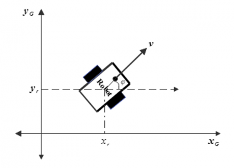
In this section, we will conduct a comprehensive analysis of the kinematics of the mobile robot, accompanied by an introduction to fundamental analytical concepts. To facilitate this analysis, Figure 3 illustrates the geometry and kinematic characteristics of the robot, providing a visual reference for better understanding.
The study of the robot's kinematics involves examining its motion without considering the forces involved. This analysis will shed light on crucial aspects such as its position, velocity, and acceleration, allowing us to grasp how the robot moves and interacts within its environment.
By providing an overview of the robot's geometry and kinematic characteristics, we aim to establish a solid foundation for comprehending its behavior and developing effective control strategies. Understanding the kinematics of the robot is instrumental in devising a successful path planning algorithm and implementing obstacle avoidance techniques.
In the forthcoming sections, we will delve further into the graphical and mathematical aspects of the robot's kinematics, enhancing our insights into its motion and enabling us to design optimized navigation algorithms for various scenarios and tasks.
As a preliminary step, we know that the sum of the attractive forces equals the total resultant forces.
Force in $x$-direction:
$F_{x \text { net }}=F_{x a t t}+F_{x r e p}$ (27)
Force in $y$-direction
$F_{\text {ynet }}=F_{\text {yatt }}+F_{\text {yrep }}$ (28)
So the resultant is:
$F_{\text {net }}=\sqrt{F_{\text {xnet }}^2+F_{\text {ynet }}^2}$ (29)
The first thing that the robot needs to do is pinpoint the location of the target, then rotate and spin it, and then knead the equation that follows.
The study of robot kinematics focuses on how robots interact with the surroundings in which they operate [20].
Figure 3. Equation of kinematics for differential drive
$v_x=V \cos \varphi, v_y=V \sin \varphi$
The angle that defines the direction of travel toward the objective is denoted by the following:
$F_{\text {net_direction }}=\tan ^{-1}\left(\frac{F_{\text {ynet }}}{F_{\text {xnet }}}\right)$ (30)
This phase includes using Newton's Second Law to locate the target place after integrating the velocity as a function of time.
$\sum F_{r o b}=m_{r o b} * \gamma_{r o b}$ (31)
After doing the calculations, we have determined the velocity in $x$.
$v_x=v * \cos \left(\left(\frac{F_{\text {ynet }}}{F_{\text {xnet }}}\right)\right)+\left(\frac{F_{\text {xnet }}}{m_{\text {rob }}}\right) * \tau$ (32)
Also, in $y$
$v_y=v * \cos \left(\left(\frac{F_{\text {ynet }}}{F_{\text {xnet }}}\right)\right)+\left(\frac{F_{\text {ynet }}}{m_{\text {rob }}}\right) * \tau$ (33)
By integrating the robot's acceleration with respect to time, we can derive functions that describe the velocity in both the $x$ and $y$ directions. These functions provide valuable insights into the robot's speed and direction of motion along the horizontal and vertical axes:
$X_{d e s}=X_{p r v}+\left(v_x * \tau\right)$ (34)
$Y_{d e s}=Y_{p r v}+\left(v_y * \tau\right)$ (35)
Our ability to achieve our goals effectively lies in our capacity to obtain the desired position and adopt a new orientation simultaneously. This capability is a pivotal reason for our success. We utilize this information to transmit relevant data to the designated node responsible for handling fuzzy logic.
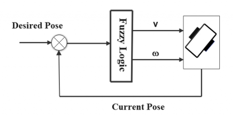
Fuzzy logic-based controllers are utilized at the basis of the design to manage the robot's path.
The path that the robot follows is directed by controllers that are based on fuzzy logic, which is located in the lowest level of the architecture as shown in Figure 4.
The model is regulated based on the polar coordinates, which results in two input membership functions for the fuzzification process. These membership functions are the error in the distance and the angle error. The linear and angular velocities of the robot are considered output functions.
Figure 4. Fuzzy logic control scheme for positional movement
After determining the necessary location and direction through orientation, the next step is to determine the necessary angular velocity and linear velocity for the robot so that it can overcome the ovoid obstacle with the fewest possible adjustments and easily reach the target without any problems
4.1 Input fuzzy sets: Distance/angle
The difference in the distance traveled by the robot between its current position and its intended destination
Fuzzy logic-based controllers are employed in the lowest level of the architecture of the robot to govern the trajectory that the robot will follow.
The fact that the model is governed by polar coordinates produces two input membership functions for the fuzzification process. These functions are errors in the distance and errors in angular orientations, and they are used to generate random values. The linear and rotational velocities of the robot both serve as output functions.
Table 1 provides a detailed description of the input fuzzy sets used in the controller of mobile robot vehicles. These fuzzy sets play a crucial role in mapping input variables to linguistic labels, enabling the robot to interpret its environment and make intelligent decisions. Fuzzy logic allows the system to handle uncertainties, making the robot adaptable in complex environments. By incorporating these fuzzy sets into the controller, the robot's navigational capabilities are enhanced, ensuring safe and efficient operations in real-world scenarios
Table 1. Input fuzzy sets distance with intervals
|
Input Fuzzy Sets: Distance |
Intervals |
|
Near |
$\left[0,0, \frac{1}{2}\right]$ |
|
Middle |
$\left[0, \frac{1}{2}, 1\right]$ |
|
Far |
$\left[\frac{1}{2}, 1\right.$, inf, inf $]$ |
This value was selected since the search space is 5 meters; however, these values are subject to modification if we decide to upgrade the search space.
In addition to this, errors in the distance input membership function have been shown in Figure 5.
Figure 5. Fuzzy set distance intervals as input
The necessary condition is that our intervals should overlap the intersection between other intervals.
The long-distance is defined as any distance greater than one.
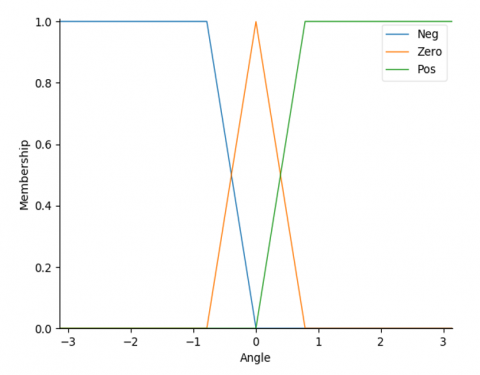
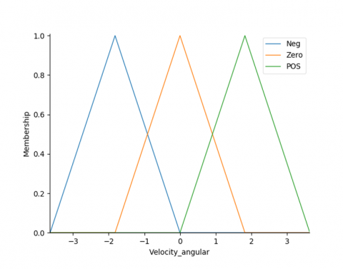
4.2 Input fuzzy sets: Angle (orientation error)
Table 2 describes the various input sets for our robot's angle.
Table 2. Angle and interval values are taken from fuzzy sets as input
|
Input Fuzzy Sets: Distance |
Intervals |
|
Neg |
$\left[-\pi,-\pi,-\frac{\pi}{4}, 0\right]$ |
|
Zero |
$\left[-\frac{\pi}{4}, 0, \frac{\pi}{4}\right]$ |
|
Pos |
$\left[0, \frac{\pi}{4}, \pi, \pi\right]$ |
The robot that we have been studying can complete a full rotation between - and. -π and π. And the representation of the error in the angle input membership function is shown in Figure 6.
Figure 6. Fuzzy set distance intervals as input
The inference system, which is utilized for the controller of Mobile Robots, has a rule base that is described in Table 3. The following are some of the variables that are contained in this Table 3.
Table 3. Robot mobile Turtlebot3 rules base
|
Angle |
Negative |
Zero |
Positive |
|
Distance |
|||
|
Near |
Linear velocity=null Angular velocity=Neg |
Angular velocity=Null Linear velocity=Null |
Linear velocity=null Angular velocity=Pos |
|
Med |
Linear velocity=null Angular velocity=Neg |
Angular velocity=Null Linear velocity=Half |
Linear velocity=null Angular velocity=Pos |
|
Far |
Angular/Linear velocity=null Angular velocity=Neg |
Angular velocity=Null Linear velocity=Full |
Linear velocity=null Angular velocity=Pos |
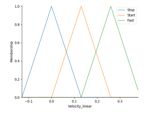
4.3 Output fuzzy sets
The inaccuracy in the robot's location is used as an input membership function for the fuzzified, while the linear velocity is used as an output function for the DE-fuzzifier. This allows for individual control of each axis description of the error in the linear output membership function of the velocity as shown in Table 4 and Figures 7 and 8.
Table 4. Fuzzy output sets for linear and angular velocities intervals
|
Linear Velocity |
Angular Velocity |
|
[-0.11, 0, 0.11] |
[-2.84, -1.42, 0] |
|
[0, 0.11, 0.22] |
[-1.42, 0, 1.42] |
|
[0.11, 0.22, 0.33] |
[0, 1.42, 2.84] |
Figure 7. Linear velocity of the output of the fuzzy sets
Figure 8. Angular velocity of the output of the fuzzy sets
4.4 Defuzzification
Defuzzification can be accomplished using a variety of techniques, some of which include the centroid, bisector, middle of maximum (MOM), smallest of maximum (SOM), largest of maximum (LOM), and others. In this particular piece of writing, we will be utilizing the centroid approach, which is also commonly referred to as the center of gravity (COG).
The essential idea behind the (COG) technique is to locate the x-coordinate of the imaginary line that, if drawn vertically, would divide the aggregate into two equal parts.
The combined control action is represented by a distribution of membership functions, the area of which is partitioned into several smaller regions. The defuzzied value, which is indicated by the notation "using COG," is defined as follows:
$x^*=\frac{\sum_{i=1}^n x_i \cdot \mu\left(x_i\right)}{\sum_{i=1}^n \mu\left(x_i\right)}$ (36)
$x_i$ represents the position (usually the output variable) along the range of the output fuzzy set, $\mu\left(x_i\right)$ stands for the membership function, and $n$ is the number of individual items that make up the sample.
In conclusion, the Intelligent Controller: Fuzzy Logic section highlights the usage of fuzzy logic graphical and linguistic variables in the mobile robot's controller. The integration of fuzzy logic enables the robot to interpret environmental inputs and navigate complex terrains while avoiding obstacles. The linguistic variables enhance decision-making capabilities by processing imprecise data. The center of gravity (COG) defuzzification method is employed to obtain precise control actions from fuzzy logic outputs. This combination of fuzzy logic and COG defuzzification results in a robust and adaptive algorithm for path planning and obstacle avoidance. The upcoming simulation results will further validate the algorithm's effectiveness in both real-time and simulated environments
5.1 Simulation nodes/parameters
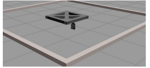
In this section, we present the results of robot simulation experiments conducted in the robot operating system (ROS) environment, utilizing the Gazebo simulation platform with the TurtleBot3 Burger robot model.
ROS is an open-source robot meta-operating system that offers comprehensive functionalities for hardware abstraction, low-level device control, and message-passing between processes. It provides a robust framework for developing and executing programs on a network of computers.
Figure 9. Robots and intended obstacles leading to goal
Gazebo, on the other hand, is a powerful ROS-enabled physical simulation environment for robots. By leveraging Gazebo within ROS, we can emulate real-world scenarios and assess the performance of the proposed algorithm in navigating through various environments with obstacles (Figure 9). The simulation results, presented through visual representations such as trajectory plots and performance metrics, provide valuable insights into the algorithm's effectiveness and potential for autonomous navigation in complex and dynamic environments
TurtleBot is a robot built on the ROS standard platform.
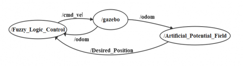
The scenario is to get the robot to move on to the next point, we first create the Fuzzy_Logic_Control Node containing control and Artificial_Potential_Field, then call the gazebo node and work with topics /Odom and /cmd_vel, and finally have the artificial potential field node publish the desired pose to the Fuzzy logic node.
Figure 10. Topics and nodes connection to move the robot to the goal
Whereas the scenario is displayed in Figure 10 with ‘odom’ for odometry information and cmd_vel for a set The velocity (both linear and angular) of a moving robot.
These investigations were carried out in Ros. The findings of the simulation are presented below in two distinct parts. In the first part of this task, our robot will go from its starting position to its destination point without encountering any obstacles. The second part of this article presents the findings obtained by the robot when navigating obstacles. Parameters upon which the fuzzy intervals we will be developing can be established may be found in Table 5, which dhow the fixed value of parameters in the simulation.
Table 5. The simulation's parameters and their values
|
Parameters |
Value |
|
Masse |
m=1 KG |
|
Q* |
1.5 m |
|
Maximum translational velocity |
0.22 m/s |
|
Maximum Rotational velocity |
2.84 rad/s |
|
$\tau$ |
10-2 s |
5.2 Result
This work describes the effective coupling of the APF approach with the fuzzy logic control methodology for path planning for mobile robots.
When the robot reaches the proper approach coordinates, both its angular and linear velocities will be brought to an absolute halt, and it will come to a complete stop once it reaches that point.
Testing the algorithm in the ROS environment serves as verification of its accuracy. Following the presentation of the results obtained using the APF approach, the results obtained using the proposed hybrid method are contrasted side by side. An obstacle is placed in the middle of the depicted Workspace.
We showcase the TurtleBot3 Burger robot's performance in a comprehensive simulation scenario depicted in Figures 11 A, B, C, and D, all set within the same environment. Throughout these simulations, the TurtleBot3 Burger effectively navigates towards its goal, skillfully evading obstacles, and adhering to the shortest path planning, thereby demonstrating its efficient and precise navigation capabilities.
In conclusion, the TurtleBot3 Burger robot successfully accomplishes its mission by intelligently selecting the path with the fewest obstacles and efficiently planning its trajectory to follow the shortest route. Moreover, the fluctuations in linear and angular velocities, which are skillfully managed by the fuzzy logic node, contribute to the robot's adaptive and responsive behavior during navigation. These results highlight the effectiveness of the proposed algorithm in achieving safe and optimal autonomous mobile robot navigation in complex and dynamic environments.
(A)
(B)
(C)
(D)
Figure 11. Embarking on success: A robot's journey overcoming obstacles along the path to goal
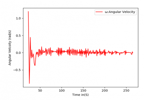
Figure 12. Change in angular velocity over time
Figure 13. Variation of liner velocity in time
In Figures 12 and 13, we present the variation of angular velocity and Linear velocity, respectively, as observed during the robot's navigation in the simulation scenarios.
In Figure 12, the plot showcases the changes in the robot's angular velocity as it manoeuvres through the environment. These fluctuations indicate the robot's ability to rotate and adjust its heading to avoid obstacles and maintain alignment with the planned path. The algorithm's intelligent control over the angular velocity allows the robot to make precise turns and navigate through tight spaces with agility.
In Figure 13, we observe the fluctuations in the robot's linear velocity throughout its trajectory. These variations are a direct result of the algorithm's adaptability to different environmental conditions and obstacle avoidance. The robot intelligently adjusts its speed based on the proximity to obstacles and the complexity of the path, ensuring smooth and efficient navigation.
Overall, the variations in linear and angular velocities demonstrated in Figures 12 and 13 affirm the efficacy of the proposed algorithm in achieving dynamic and responsive navigation. The ability to adapt speed and heading to the surroundings ensures the TurtleBot3 Burger's safe and efficient movement while successfully avoiding obstacles and adhering to the shortest path planning. These velocity profiles reinforce the algorithm's capacity to handle diverse scenarios and validate its suitability for real-world applications in autonomous robot navigation.
In conclusion, this research presents an algorithm for autonomous mobile robot navigation that addresses the challenges of obstacle avoidance and efficient path planning. By combining the enhanced artificial potential field (APF) technique with fuzzy logic control (FLC), we have achieved remarkable results in guiding the TurtleBot3 Burger robot through complex and dynamic environments.
The proposed algorithm successfully enables the robot to navigate from an initial point to a goal point while effectively avoiding collisions with both static and obstacles. The use of APF provides a magnetic and repulsive force model, allowing the robot to be attracted to its goal while being repelled from obstacles, leading to smooth and continuous trajectories. Fuzzy logic control enhances the adaptability of the robot, allowing it to dynamically adjust its linear and angular velocities based on the environmental conditions, ensuring safe and responsive navigation.
The simulation results have demonstrated the algorithm's efficiency in finding the shortest and safest path to the goal while avoiding collisions. The ability of the TurtleBot3 Burger robot to navigate through dense and closely spaced obstacles with precision reaffirms the algorithm's robustness and suitability for real-world applications.
The analysis of linear and angular velocity variations during navigation further highlights the algorithm's intelligent control over the robot's movement. These velocity profiles demonstrate the algorithm's adaptability to different scenarios, making it an effective and reliable solution for autonomous mobile robot navigation.
While this research has achieved promising results, there are still areas for further improvement and exploration. Future research may focus on optimizing the algorithm's computational efficiency, extending it to handle more complex environments, and integrating additional sensor modalities for enhanced perception and decision-making.
In conclusion, the developed algorithm opens up new possibilities for autonomous mobile robots to safely and efficiently navigate through challenging environments, bringing us closer to the realization of intelligent and autonomous robotic systems that can operate seamlessly in real-world scenarios.
|
$l_{\text {goal }}, d_{\text {obstacle }}$ |
Distance: Meters (m) |
|
|
$F_{a t t}, F_{r e p}, F_{\text {net }}$ |
Force: Newtons (N), $N=1 \mathrm{~kg} \mathrm{~m} \mathrm{~s}^{-2}$ |
|
|
$k_{a t t,} k_{r e p}$ |
Gain parameters |
|
|
$v$ |
Linear Velocity in m.s-1 |
|
|
$\omega$ |
Angular velocity rad.s-1 |
|
|
$\gamma$ |
gravitational acceleration, m.s-2 |
|
|
$m_{r o b}$ |
Mass: Kilograms (kg) |
|
|
$X_{\text {des }}, Y_{\text {desired }}$ |
Length: Meters (m) |
|
|
$\tau$ |
Time: Seconds (s) |
|
|
$Q^*$ |
Safe Distance in m |
|
|
Greek symbols |
||
|
$\mu\left(x_i\right)$ |
Stands for the membership function |
|
|
n |
The number of individual items |
|
|
$x_i$ |
Solid volume fraction |
|
|
$\varphi$ |
Orientation angle |
|
|
Subscripts |
||
|
APF |
Artifital Potenteil Fieald |
|
|
FLC |
Fuzzy Logic Control |
|
|
ROS |
Robot Operating System |
|
|
MOM |
Middle Of Maximum |
|
|
SOM |
Smallest Of Maximum |
|
|
SOG |
Center Of Gravity |
|
|
LOM |
Largest Of Maximum |
|
[1] Li, G., Tamura, Y., Yamashita, A., Asama, H. (2013). Effective improved artificial potential field-based regression search method for autonomous mobile robot path planning. International Journal of Mechatronics and Automation, 3(3): 141-170. http://doi.org/10.1504/IJMA.2013.055612
[2] Azzabi, A., Nouri, K. (2017). Path planning for autonomous mobile robot using the Potential Fiels method. In 2017 International Conference on Advanced Systems and Electric Technologies (IC_ASET): Hammamet, Tunisia. http://doi.org/10.1109/ASET.2017.7983725
[3] Chancharoen, R., Sangveraphunsiri, V., Navakulsirinart, T., Thanawittayakorn, W., Boonsanongsupa, W., Meesaplak, A. (2002). Target tracking and obstacle avoidance for mobile robots. In 2002 IEEE International Conference on Industrial Technology, Bankok, Thailand, pp. 13-17. http://doi.org/10.1109/ICIT.2002.1189851
[4] Khatib, O. (1985). Real-time obstacle avoidance for manipulators and mobile robots. In Proceedings. 1985 IEEE International Conference on Robotics and Automation, St. Louis, MO, USA, pp. 500-505. https://doi.org/10.1109/ROBOT.1985.1087247
[5] Rostami, S.M.H., Sangaiah, A.K., Wang, J., Liu, X. (2019). Obstacle avoidance of mobile robots using modified artificial potential field algorithm. EURASIP Journal on Wireless Communications and Networking, 2019(1): 1-19. http://doi.org/10.1186/s13638-019-1396-2
[6] Yan, P., Yan, Z., Zheng, H., Guo, J. (2018). Real time robot path planning method based on improved artificial potential field method. In 2018 37th Chinese Control Conference (CCC), Wuhan, China, pp. 4814-4820. https://doi.org/10.23919/ChiCC.2018.8482571
[7] Xie, S., Wu, P., Peng, Y., Luo, J., Qu, D., Li, Q., Gu, J. (2014). The obstacle avoidance planning of USV based on improved artificial potential field. In 2014 IEEE International Conference on Information and Automation (ICIA), Hailar, China, pp. 746-751. http://doi.org/10.1109/ICInfA.2014.6932751
[8] H. Nguyen, P.D., Recchiuto, C.T., Sgorbissa, A. (2018). Real-time path generation and obstacle avoidance for multirotors: A novel approach. Journal of Intelligent & Robotic Systems, 89: 27-49. https://doi.org/10.1007/s10846-017-0478-9
[9] Chen, Y., Peng, H., Grizzle, J. (2017). Obstacle avoidance for low-speed autonomous vehicles with barrier function. IEEE Transactions on Control Systems Technology, 26(1): 194-206. http://dx.doi.org/10.1109/TCST.2017.2654063
[10] Miller, L., Toal, D., Omerdic, E., Dooly, G., Coleman, J., Duffy, G. (2012). Low cost navigation for unmanned underwater vehicles using line of soundings. IFAC Proceedings Volumes, 45(5): 63-68. http://doi.org/10.3182/20120410-3-PT-4028.00012
[11] Van, M., Do, X.P., Mavrovouniotis, M. (2020). Self-tuning fuzzy PID-nonsingular fast terminal sliding mode control for robust fault tolerant control of robot manipulators. ISA Transactions, 96: 60-68. https://doi.org/10.1016/j.isatra.2019.06.017
[12] Fang, M.C., Wang, S.M., Mu-Chen, W., Lin, Y.H. (2015). Applying the self-tuning fuzzy control with the image detection technique on the obstacle-avoidance for autonomous underwater vehicles. Ocean Engineering, 93: 11-24. http://doi.org/10.1016/j.oceaneng.2014.11.001
[13] Elkilany, B.G., Abouelsoud, A.A., Fathelbab, A.M., Ishii, H. (2020). Potential field method parameters tuning using fuzzy inference system for adaptive formation control of multi-mobile robots. Robotics, 9(1): 10. http://doi.org/10.3390/robotics9010010
[14] Ren, L.M., Wang, W.D., Du, Z.J. (2021). A new fuzzy intelligent obstacle avoidance control strategy for wheeled mobile robot. In 2012 IEEE International Conference on Mechatronics and Automation, Chengdu, China, pp. 1732-1737. https://doi.org/10.1109/ICMA.2012.6284398
[15] Smith, S.M., Rae, G.J.S., Anderson, D.T. (1993). Applications of fuzzy logic to the control of an autonomous underwater vehicle. In Proceedings 1993 Second IEEE International Conference on Fuzzy Systems, San Francisco, CA, USA, pp. 1099-1106. http://doi.org/10.1109/FUZZY.1993.327361
[16] DeMuth, G., Springsteen, S. (1990). Obstacle avoidance using neural networks. In Symposium on Autonomous Underwater Vehicle Technology, Washington, DC, USA, pp. 213-215. http://doi.org/10.1109/AUV.1990.110459
[17] Wang, J.S., Lee, C.G. (2003). Self-adaptive recurrent neuro-fuzzy control of an autonomous underwater vehicle. IEEE Transactions on Robotics and Automation, 19(2): 283-295. https://doi.org/10.1109/TRA.2003.808865
[18] Joseph, L., Cacace, J. (2021). Mastering ROS for Robotics Programming: Best Practices and Troubleshooting Solutions when Working with ROS, Packt Publishing.
[19] Pyo, Y., Cho, H., Jung, R.W., Lim, T. (2017). ROS Robot Programming. https://www.robotis.us/ros-robot-programming-book/.
[20] Mhanni, Y., Lagmich, Y. (2023). Implementation of artificial potential fields and lyapunov stability and control in obstacles avoidance of mobile robot using ros gazebo. Journal of Theoretical and Applied Information Technology, 101(4): 1184-1193.