Tulus*![]() | Md Mustafizur Rahman
| Md Mustafizur Rahman![]() | Sutarman
| Sutarman![]() | Muhammad Romi Syahputra
| Muhammad Romi Syahputra![]() | Tulus Joseph Marpaung
| Tulus Joseph Marpaung![]() | Jonathan Liviera Marpaung
| Jonathan Liviera Marpaung![]()
© 2023 IIETA. This article is published by IIETA and is licensed under the CC BY 4.0 license (http://creativecommons.org/licenses/by/4.0/).
OPEN ACCESS
Wave propagation, a phenomenon involving the transfer of energy over time, is a significant area of study, particularly with respect to sea waves. Due to their unique geometrical properties and inhomogeneous minimum amplitude, sea waves pose distinct challenges for numerical solutions. This research focuses on the analysis of wave stability against various water velocities and breakwater distances from the coastline. The study employs a hybrid approach, utilizing the Finite Element Method (FEM) to determine the movement of fluid elements through a porous, submerged breakwater. The concept of permeability in breakwaters is integral to this analysis. Permeable breakwaters permit a certain proportion of seawater or wave water to pass through, while absorbing or reflecting the remaining component of the waves. Understanding the permeability of breakwaters can enhance the design effectiveness and efficiency, whilst providing insight into potential impacts on coastal ecosystems. The results of the study demonstrate that the distance of the breakwater from the incoming wave influences both the amplitude and speed of the wave. Specifically, a greater distance between the wave and the breakwater results in a decrease in wave height, thereby increasing the stability of the simulation. For example, the directional and speed components of the movement at [x, y, t] for the first amplitude [20, 2, 15] was found to be 0.12515m, the second amplitude [15, 2, 15] 0.13161m, and the third amplitude [10, 2, 15] 0.13097m. This demonstrates that the breakwater's distance significantly influences wave stability, an important factor to consider in future breakwater design and implementation.
breakwater, simulation, fluid dynamics, h-fem, partial differential equations
A wave refers to a traveling vibration that moves through a medium or a collection of interconnected objects. Practical instances of waves are observable in scenarios involving surface waves, like ocean waves approaching a shoreline. The undulations on the water’s surface result from the interplay between moving air masses and the upper layer of the water, forming a pattern of crests and troughs influenced by energy and momentum. Essentially, surface water waves emerge not solely from air movement but can also arise from various actions occurring at the water’s depths. Researches [1, 2] elucidat that the speed at which surface water waves propagate is contingent upon factors such as surface tension, hydrostatic pressure, water depth, mass density, and gravity. Several factors contribute to the generation of water surface waves, including wind currents and vibrations originating from the water’s depths, exemplified by occurrences like tsunami waves.
Peng et al. [3] conducted a study on how to reduce the strength of waves at sea level using a breakwater in the form of a porous block. The first thing to do in this research is to form a wave model of the surface of the water through a breakwater in the form of a porous block. The formation of the model involves utilizing the fundamental equations governing the passage of surface waves through porous beams. These equations encompass the continuity equation, momentum equation, potential wave velocity, considerations of fluid within porous media, as well as Laplace and Bernoulli equations within both fluid and porous contexts. Moreover, kinematic and dynamic boundary conditions are imposed at the fluid surface [4]. The resultant model bears remarkable resemblance to the shallow water equation. The subsequent steps outlined in references [5-7] elucidate the process of obtaining a numerical solution from this established model. The numerical solution is attained through the finite difference method, employing an implicit scheme corrector and predictor. The study’s findings reveal that the amplitude of the wave diminishes subsequent to interaction with the breakwater. The extent of wave attenuation hinges on factors such as the quantity and height of breakwaters. For solving diverse types of differential equations, one viable approach is the employment of the boundary element method, which is grounded in Taylor series expansion principles [8, 9].
Research on breakwaters aims to determine the phenomena that occur with the energy generated from the movement of seawater towards coastal areas, which are shallow areas [10]. The development of research on breakwaters has been carried out by several mathematicians and physicists who focus on breakwater models [11]. In the research that has been done, breakwaters with different dimensions will produce different results according to the specified model parameters. In terms of optimizing the breakwater model, it is influenced by several important parameters such as the wave velocity, wave height, depth, pressure, and even Newtonian force, which results in momentum in the breakwater [12, 13]. Huang et al. [14] explained how the analysis of the interaction between models of breakwaters used in three-dimensional problems with porous breakwater models by developing equations from the Navier-Stokes equations resulted in a 3D wave propagation model for surface-emerging breakwaters.
Many simulations of breakwaters have been carried out to find out how much wave reduction is produced by both the speed and wave height values [15]. Simulation involving different parameters will give complex results in its completion because it is necessary to use a multi-purpose programming model [16]. The results of research with a focus on wave propagation stability analysis [17] need to consider the magnitude of the reduction of the incident wave so that the amplitude value delivered to the shallow area is at a steady state point.
Researches on the stability of wave propagation have been carried out [18, 19] to determine the factors that affect stability in wave propagation in terms of wave propagation reliability, breakwater reliability, and also the probability density function (PDF) value. The resulting impact of large waves is damage to shallow areas and even coastal areas, which are critical areas [20]. The optimal wave splitting process aims to reduce the magnitude of wave resonance at the harbor by applying the Helmholtz equation, which has complex values as the model state equation with minimizing wave amplitude as the optimization variable [21].
The author proposes that a water wave breakwater will provide momentum resistance to subsurface currents so that the amount of momentum that occurs will be reduced at the bottom of the shallow area before the wave propagates to the coastal area [22]. The results to be achieved from this study are simulations of wave height ($\lambda$) from variations in the depth of the breakwater position from the sea surface. This study will also simulate the effect of speed variations on the amplitude of the waves that occur. The formation of a breakwater model will be carried out by testing the reliability of moving against time to reach the stability area against the variations in constraints that are carried out. In this study, the authors will simulate wave breaking using a submerged porous breakwater to find a numerical solution using the Hybrid Finite Element Method (HFEM) is a computational technique that integrates the attributes of many finite element techniques.
2.1 Breakwater simulation
Submersible breakwaters are facilities built to break waves under the surface of the water with the aim of dampening and absorbing internal energy from wave propagation underwater. Based on the principle of hydrostatic pressure, the greatest water pressure is at the bottom of the sea, which is expressed by the pressure of water directly proportional to the depth of the sea. Hydrostatic pressure is expressed as:
$-\delta P=q \rho \delta z$ (1)
where, $\lim _{\delta z \rightarrow 0}-\delta P$ and the Eq. (1) can be expressed as:
$\frac{\partial P}{\partial z}=g \rho$ (2)
where, $P, g, \rho, \partial z$ respectively represent hydrostatic pressure, gravitational acceleration, fluid density, and changes in water depth [23]. Eq. (1) is written with a negative sign with the assumption that the pressure P will decrease with increasing height which is applied to the problem of hydrostatic pressure in the case of an object moving towards the atmosphere.
For the submerged breakwater problem, Eq. (1) will be an increase in $\partial z$ which will result in an increase in pressure P so that the pressure will be greater in the bottom area. The submerged breakwater will absorb some of the energy from the bottom area with the aim of reducing the amount of energy that is in the surface area. An illustration of the wave breaking process with a breakwater is shown in Figure 1.
Figure 1. Submerged permeable breakwater simulation
The breakwater will absorb some of the inner energy at the bottom of the wave by releasing the wave propagation that hits the breakwater, so that a process of changing momentum occurs in the wave propagation [24]. The process of breaking waves with a submerged type is often used to control large-scale wave propagation for coastal areas or port areas, which maintain the magnitude of wave propagation in coastal areas. The permeability of rocks to wave barriers exhibits significant variability, which is contingent upon several parameters, including rock type, rock size and form, and the spatial arrangement of rocks. Permeability refers to the inherent capacity of a medium to facilitate the passage of fluids or waves. In order to elucidate the permeability characteristics of a wave breaker, it is important to acknowledge the existence of several kinds of waves, including water waves and seismic waves and earthquake occurred.
The usage of rock formations as wave breakers is a common practice that capitalizes on the mechanical and acoustic characteristics of the rocks. The configuration of rocks is often engineered to mitigate the impact of water waves, such as in coastal regions, where it serves as a protective measure against storm waves or tempestuous conditions. Conversely, stone arrangements may serve the purpose of mitigating the effects of earthquakes through the strategic redirection of seismic waves. The permeability of the wave-breaker should be neither too high nor excessively low. In the event that the permeability is excessively elevated, the waves possess the capacity to traverse the wave-breaker with little impedance to achieve the intended outcome.
In the event of poor permeability, the wave breaker may effectively mitigate wave activity, although it might concurrently induce heightened hydrostatic pressure on the breaker structure, potentially resulting in detrimental consequences such as rock damage or displacement. The measurement of wave breaker permeability often employs units that align with the specific wave type targeted for obstruction. In the context of water waves, the measurement of permeability is often expressed in units of meters per second (m/s) or something comparable. The measurement of permeability in seismic waves may be determined by considering the dimensions of the rock and the coefficient of rock elasticity.
2.2 Navier-Stokes equation on moving fluids
The Navier-Stokes equation constitutes a mathematical framework that addresses fluid-related challenges pertaining to both fluid substances and the attributes intrinsic to them [25-27]. The modeling inherent in the Navier-Stokes equation delineates the manner in which the velocity vector’s magnitude evolves across the u and v components as they traverse the x and y coordinates over time. In scenarios involving vector analysis, it is established that all attributes of the fluid are contingent upon spatial dimensions and temporal evolution. These attributes can be exemplified by vector quantities like velocity (v) and acceleration (a). Let a is a vector component of velocity and time vector that can be written as:
$\vec{a}=\left(\frac{d u}{d t}, \frac{d v}{d t}\right)$ (3)
denote that $\vec{a}=\frac{d \vec{v}(x, y, t)}{d t}$, consists of components in Eq. (3), then by following the chain rule then the value of $\vec{a}$ for each component is:
$\vec{a}_x=\frac{d u}{d t}=\frac{\partial u}{\partial t}+\frac{\partial u}{\partial x} \frac{d x}{d t}+\frac{\partial u}{\partial y} \frac{d y}{d t}$ (4)
$\vec{a}_y=\frac{d v}{d t}=\frac{\partial v}{\partial t}+\frac{\partial v}{\partial x} \frac{d x}{d t}+\frac{\partial v}{\partial y} \frac{d y}{d t}$ (5)
For each value of $\frac{d x}{d t}, \frac{d y}{d t}$ is a function of space against time which can be written respectively as $u, v$ which results in the acceleration value in Eq. (4) and Eq. (5) for each component are:
$\vec{a}_x=\frac{d u}{d t}=\frac{\partial u}{\partial t}+\vec{v} \cdot \nabla u$ (6)
$\vec{a}_y=\frac{d v}{d t}=\frac{\partial v}{\partial t}+\vec{v} \cdot \nabla v$ (7)
Simply, the vector of a can be written as:
$\vec{a}=\left(\frac{\partial}{\partial t}+\vec{v} \cdot \nabla\right) \vec{v}$ (8)
2.3 Hybrid Finite Element Method
In general, the combination of Finite Element Method (FEM) and Boundary Element Method (BEM) offers a robust methodology for the examination of intricate geometric quandaries, facilitating a more comprehensive comprehension of the dynamics exhibited by physical systems. Both approaches provide distinct benefits and may synergistically enhance one another to yield precise and effective answers. The finite element approach divides the problem domain into smaller, non-uniform components. This feature facilitates the representation of intricate or non-uniform geometry. The boundary element method is a numerical technique that operates specifically on the borders of a given domain. Hence, the Boundary Element Method (BEM) is highly suitable for the analysis of modeling challenges that include infinite or extensive bounds.
The combination of the Finite Element Method (FEM) and the Boundary Element Method (BEM), known as FEM-BEM or Hybrid FEM, offers a viable approach for addressing complex issues. This methodology involves partitioning the domains into smaller subdomains using FEM, then afterwards using BEM to investigate the interactions between these subdomains. By leveraging this hybrid approach, it becomes possible to effectively tackle large-scale problems. The Hybrid Finite Element Method is used to determine the initial value of a function that moves with time [28, 29]. The equation using Hybrid Finite elements will provide an efficient solution by separating the wave equation from the momentum equation and then linearizing [30].
$\int_0^{t_f^{+}} \int_0^r\left(\frac{\partial^2 \eta}{\partial t^2}-c^2 \frac{\partial^2 \eta}{d x^2}\right) \eta^* d x d t=\int_0^{t_F^*} \int_0^c B \eta^* d x d t$ (9)
where, $r$ is the region length and $t_F^{+}=t_F+\epsilon$, where $\epsilon$ is a small arbitrary parameter [31]. In the above expression $Z^*$ is the fundamental solution of the one-dimensional wave operator, given by:
$\eta^*=-\frac{1}{2 C} H\left[c\left(t_F-t\right)-r\right]$ (10)
in which H is the Heaviside function and $r=\|x-s\|$, s and x indicating the source and field point positions respectively. Integrating the second-order derivatives in Eq. (5) twice by parts, the following equation is obtained:
$\begin{gathered}\int_0^{t_f^{+}} \int_0^r\left(\frac{\partial^2 \eta^*}{\partial t^2}-c^2 \frac{\partial^2 \eta}{d x^2}\right) \eta d x d t+\int_0^r\left[\eta^* \frac{\partial \eta}{\partial t}-\right. \left.\eta \frac{\partial \eta^*}{\partial t}\right]_0^{t_F^*} d x-c^2 \int_0^{t_F^*}\left[\eta^* \frac{\partial \eta}{\partial x}-\eta \frac{\partial \eta^*}{\partial x}\right]_0^r d t= \int_0^{t_F^{+}} \int_0^r B \eta^* d x d t\end{gathered}$ (11)
Wave transmission $\left(H_t\right)$ refers to the magnitude of the wave that successfully passes beyond an obstruction and is determined by the transmission coefficient $\left(K_t\right)$, computed using the subsequent formula:
$K_t=\frac{H_t}{H_i}=\sqrt{\frac{E_t}{E_i}}$ (12)
In this equation, $K_t$ represents the wave transmission, $K_i$ stands for the reflected wave, $H_t$ embodies the value of $H_t$ achieved by multiplying $K_t$ with $H_i$ (where $H_i$ signifies the initial wave height). Additionally, $E_t$ denotes the transmitted energy, while $E_i$ signifies the incoming energy. The calculation of transmitted wave energy, $E_t$ is given by the expression $E_t=\frac{1}{8} \rho g H_t$, where $\rho$ denotes fluid density and g signifies gravitational acceleration.
Theorem Given J and h as the proposition function $f, g$ for $\left[u_0, v_0\right] \in$ $H_0^1(\Omega) \times L^2(\Omega)$ there exists a unique function $J \times \Omega \rightarrow \mathbb{R}$ that satisfies the equation.
$\frac{\partial^2 u}{\partial t^2}-\Delta u+f(u)+g\left(\frac{\partial u}{\partial t}\right)=h(t, x) \in C\left(J, H^{-1}(\Omega)\right)$
That fulfills the condition $v=$ value $\varepsilon \in C^1(J)$ and all $t \in J$.
$\frac{d}{d t}(\varepsilon(t))=\int_{\Omega}\left[h(t, x)-g\left(\frac{\partial u}{\partial t}(t, x)\right)\right] \frac{\partial u}{\partial t}(t, x) d x$ (13)
Proof. The outcome arising from the presence of distinct values is evident within the overarching framework of the traditional approach, wherein the classical method converges with preliminary estimation mapping over the widest possible range. To be more precise, this occurs when the configuration is established. $J_\delta \cap[-\delta, \delta]$ for each $\delta>0$ for all $P>$ sup $\left\{u_0, v_0\right\}$, The set $X$ endowed with the topology of $C\left(J_\delta, V\right) \cap C^1\left(J_\delta, H\right)$ is a complete metric space, for the value $v \in X$, given $C(v)$ is the unique solution of $z \in C\left(J_\delta, V\right) \cap$ $C^1\left(J_\delta, H\right) \cap C^2\left(J_\delta, V^{\prime}\right)$ from the problem:
$\frac{\partial^2 z}{\partial t^2}-\Delta z=h(t, x)-f(v)-g\left(\frac{\partial v}{\partial t}\right)$ (14)
$z(0)=u_0, \frac{\partial z}{\partial t}(0)=v_0$ (15)
Some authors stated that the Hybrid Finite Element Method (HFEM) is a computational technique that integrates the attributes of many finite element techniques (FEM) in order to address intricate engineering and physics issues. This methodology has been developed with the intention of capitalizing on the benefits offered by each individual element technique, thereby enhancing accuracy, efficiency, and the capacity to address diverse issue scenarios. Finite Element Methods (FEMs) are used for the resolution of issues occurring in open domains or volumes, while Boundary Element Methods (BEMs) are utilized for the resolution of problems specifically on domain borders. Instances of its use may be seen in the realm of underwater structural vibration analysis, wherein Finite Element Methods (FEMs) are employed to scrutinize interior structures, such as ships, while Boundary Element Methods (BEMs) are utilized to simulate the impact of the encompassing water.
Based on the derivation of the unhindered homogeneous wave equation model in Eq. (15), a wave equation model will be formed with the damping of the breakwater, which is influenced by external forces that inhibit the propagation of water waves, namely the breakwater [18]. The wave damping process is assumed to be a modified form of the equation model by giving a negative value to the wave acceleration $\left(-u_{t t}\right)$. The magnitude of the negative acceleration illustrates that the external force has a direction opposite to the direction of wave propagation, which will result in a decrease in wave height $(\lambda)$ and a decrease in speed $\left(u_t\right)$ [32, 33]. Then based on the general homogeneous wave equation can be rewritten as:
$-u_{t t}-c u_{x x}=P_x(t) \rightarrow u_{t t}+c u_{x x}=-P_x(t)$ (16)
Eq. (16) is solved by using the separating variable method on the interval $x(0, L)$, with the initial conditions $u(x, 0)$, $u_t(x, 0)=\psi(x)$ and $u(0, t)=u(L, t)=0$. Then the solution of the homogeneous wave equation separator method is $u_{t t}=$ $-c^2 u_{x x}, \quad$ with $\quad 0<x<L, u(0, t)=u(L, t)=0, \forall t \geq 0$, $u(x, 0)=\phi(x)$, with $u_t(x, 0)=\psi(x)$, Furthermore, for the equation $u(x, t)$ it can be written that $u_{t t}=X(x) T^{\prime \prime}(t)$ and $u_{x x}=X^{\prime \prime}(x) T(t)$, then the $u_{t t}$ equation, when substituted into the separable equation above, can be written as:
$u_{t t}=-c^2 u_{x x} \leftrightarrow X(x) T^{\prime \prime}(t)=-c^2 X^{\prime \prime} T(t)$ (17)
$\frac{T^{\prime \prime}(t)}{c^2 T(t)}=-\frac{X^{\prime \prime}(x)}{X(x)}$
The solution to solving Eq. (17) is for the problem $k=\mu^2=$ $\left(\frac{n \pi}{L}\right)^2$, it can be written that $\lambda_n=\frac{c n \pi}{l}$. So, if the $\lambda_n$ value is substituted into Eq. (17) it will produce:
$u(x, t)=\sum_{n=1}^{\infty} u_n(x, t)=\sum_{n=1}^{\infty}\left\{\left(A_n+B_n\right) \cos (t)+\left(A_n-B_n\right) \frac{c n \pi}{L} \sin (t)\right\} \sin \frac{n \pi}{L} x$ (18)
It can be concluded that Eq. (18) is a homogeneous equation in the interval $0<x<L$. That can be written as:
$u(x, 0)=\sum_{n=1}^{\infty}\left(A_n+B_n\right) \sin \frac{n \pi}{L} x=\phi(x)$ (19)
3.1 Research process
To achieve accurate simulations of wave retention, the study employs a sequence of computer-based analytical techniques rooted in the optimization process for wave retardation. Utilizing the boundary element approach to obtain both elemental and comprehensive solutions for a model function, the investigation delves into the general equation concerning wave retardation versus permeable wave-breakers, as documented in existing literature. The outcome is a computational exploration that contrasts the wave model against a stable permeable wave-breaker, showcasing a simulation depicting a notably rapid reduction in wave height.
The comprehensive examination of shallow water waves involves multiple phases. These encompass discretizing the general water wave equation, as well as determining the initial values and boundary conditions of the model. Subsequently, the wave equation needs to be modified to incorporate breakwater variables aimed at inducing a negative sea wave acceleration $\left(-u_{t t}\right)$. This accounts for the opposing resistance of sea water, intended to counteract the wave’s direction and reduce values associated with wavelength $(\lambda)$, wave velocity $(v)$, and wave momentum $P_x(t)$.
Once the modified wave equation involving a seawater breakwater is established, the subsequent step involves conducting simulations. This is accomplished by employing the boundary element method and the hybrid finite element approach (Finite Element Method) through COMSOL Multiphysics 5.6 within the domain of the breakwater model. This simulation yields a representation of amplitude, velocity, and energy distribution across various iterations of propagation scenarios.
3.2 2D shallow water wave modelling
If a crash, explosion, or load as a result of an earthquake occurs, a time-dependent signal is produced and transmitted across the medium as a wave (voltage). Typically, this kind of wave moves in all three directions of space. Under certain circumstances and presumptions, idealizing such a medium as a one-dimensional medium is equivalent to supposing that a large ocean has the same depth of penetration. The wave that slows down in the bar will travel back and forth according to the way it relies on time. Assume that the wind that is always blowing over the sea surface is the type that works on the moving wave by looking at the little wave pieces on the surface. (i.e., from point x to x+Δx) on the axis x (see Figure 2).
Figure 2. Projection of wave force
The differential equation of the ocean waves may be found (at the gap $(x, x+\Delta x))$ by assuming the newtonian force that operate on the section of the sea surface. On the ocean's surface, there are curving lines that show a tense style. The projections of the $F_1 \cos \alpha$ and $F_2 \cos \alpha$ on the $x$-axis, when the $F_1$ operates on the $P$-point and the $F_1 \cos \beta$ and $F_2 \cos \beta$ operates at the $Q$-point. The forces that function in the horizontal direction should not change since everything on the surface travels vertically and nothing else. So, $F_1 \cos \alpha=$ $F_2 \cos \beta=F$ by applying the style's outcome on the $x$-axis forces projection rule. Next, the projection of the forces on the $y$-axis is $-F \sin \alpha$ and $F_2 \sin \beta$. If the speed of change occurs, it can be written that:
$F_2 \sin \beta-F_1 \cos \alpha=\rho \cdot \Delta x \cdot u_{t t}$ (20)
The product of $\rho \Delta x$ corresponds to the mass of a portion of seawater, while $u_{t t}$ denotes the second order derivative of the object’s position, representing the acceleration magnitude of the entity. From the Eq. (20), it can be written that:
$\tan \beta-\tan \alpha=\frac{\rho \Delta x}{F} \cdot u_{t t}$ (21)
The gradients on $x$ and $x+\Delta x$ are represented by the values of $\tan \beta$ and $\tan \alpha$, respectively. This can be expressed as $\tan \alpha=u_x(x, t)$ and $\tan \beta=u_x(x, x+\Delta x)$. This relationship can be formulated as follows:
$\begin{gathered}\tan \beta-\tan \alpha=\frac{\rho \Delta x}{F} \cdot u_{t t} \\ u_x(x, x+\Delta x, t)-u_x(x, t)=\frac{\rho \Delta x}{F} \cdot u_{t t} \\ \therefore \frac{1}{\Delta x}\left[u_x(x, x+\Delta x, t)-u_x(x, t)\right]=\frac{\rho}{F} \cdot u_{t t}\end{gathered}$ (22)
For $\Delta x \rightarrow 0$, the function bounded at $\lim _{\Delta x \rightarrow 0} \frac{1}{\Delta x}\left[u_x(x, x+\Delta x)-u_x(x, t)\right]=u_{x x}$, then it can be written that $u_{x x}=\frac{\rho}{F} \cdot u_{t t}$, so that it may be simplified to $c^2=\frac{F}{\rho}$.
In building a simulation of wave propagation towards a breakwater, it is necessary to initialize the wave model by determining the geometry of the wave model. At this stage a 2D wave model will be formed using COMSOL Multiphysics 5.6 as shown in Figure 3.
Figure 3. Breakwater geometry model
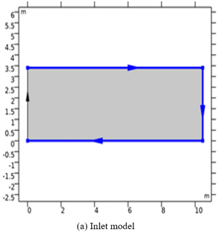
Figure 4. Boundary condition for inlet and outlet model
In the wave model, the sides that will be the inlet and outlet will be defined with the boundary conditions of each domain.
The breakwater model walls in Figure 4, is formed with geometric constraints.
$\begin{gathered}\boldsymbol{u} \cdot \boldsymbol{n}=0 \\ -\Gamma_h \cdot \boldsymbol{n}=0 \\ -\Gamma_h \cdot \boldsymbol{n}=g \frac{h^2}{2}\end{gathered}$ (23)
where, the $\boldsymbol{u}$ and $\boldsymbol{n}$ vectors denote the velocity values at the coordinates $u(x, y, t)$ and the momentum of the flux geometry model, respectively. The $\boldsymbol{\Gamma}_h$ value is the magnitude of the flux conservation of the momentum at each coordinate with the calculation for each coordinate being $\boldsymbol{u}_x \cdot \boldsymbol{q}_x+\frac{g h^2}{2}$.
In the process of meshing the model with finite elements, it was found that the size of the elements formed was 185,845 with 1,772 edges, this resulted in the need for computation in the wave model iteration so as to produce a large change in the value of the wave propagation with respect to time. In the simulation carried out, the research will test how the effect of speed on the distribution of wave velocity values after wave attenuation with each speed of 1m/s, 1.5m/s, 2m/s. Furthermore, the simulation will be continued with the modification of the breakwater model to the position length of the breakwater with a distance of 10m, 15m and 20m respectively.
Figure 5 shows the wave breaking process with a submerged breakwater model that has permeable properties and propagates in shallow water. The magnitude of the velocity fraction each time is shown in Figure 5 shows the propagation of waves that propagate after a break occurs using a porous submerged breakwater. The amplitude is generated against time and oscillates up to the outlet of the propagation area. The convergence of the wave amplitudes shows that the waves resulting from the wave splitting process show significant results, with as many as 4,836 iterations during t=[0, 15].
Figure 5. Breakwater simulation
Figure 6 shows the solution of the speed of wave propagation at t=[0, 10] with the color representation showing the critical area experiencing the greatest velocity. Furthermore, the representation of the stability of wave propagation will be shown in Figure 7.
Figure 7 shows the propagation of waves that propagate after a break occurs using a porous submerged breakwater. The amplitude is generated against time and oscillates up to the outlet of the propagation area. The convergence of the wave amplitudes shows that the waves resulting from the wave splitting process show significant results with as many as 4,836 iterations during t=[0, 10]. The resolution of the wave amplitude to the elements is shown in Figure 8.
Figure 6. Simulation of the velocity of the breakwater breaking process
Figure 7. Water wave amplitude breaking
Figure 8. Wave amplitude simulation in the wave breaking process
The completion iteration is carried out for 4.386 for t=[0, 15]. Figure 8 shows that the muted water waves show a very critical amplitude before and after the wave breaking process is carried out, the convergence of the water waves shows that the amplitude on the outlet side becomes lower in the simulation so this shows that the wave breaking process will provide amplitude attenuation and wave propagation speed the minimum. For parameter variations, a simulation is carried out on differences in wave propagation velocity of 1m/s, 1.5m/s, 2m/s to see differences in the distribution of wave speed and amplitude, then the breakwater distance parameter with a constant arrival speed of 1m/s shown in Figure 9.
Figure 9. Resistance of breakwaters to changes in speed
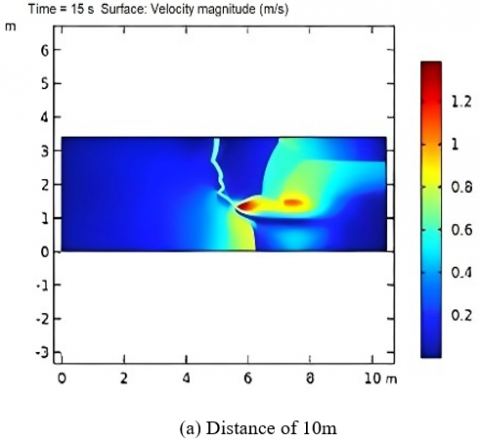
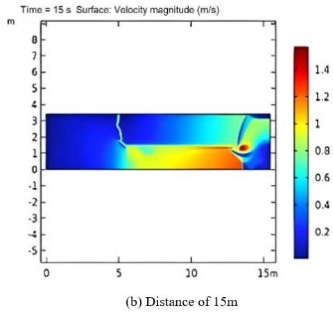
The breakwater will dampen the waves and break the wave propagation at each coordinate. Changes in the conservation of momentum will result in a change in the velocity value for each component at the coordinates $u(x, y, t)$. The magnitude of the change in velocity that occurs will have an impact on the final velocity of the wave amplitude. The offshore simulation of the breakwater was carried out by modifying the geometry model of the breakwater with constant incoming wave velocity v for distance variations of 10m, 15m, and 20m. The difference in the position of the breakwaters gives a different wave distribution. The model of the breakwater with changing distances is shown in Figure 10.
Figure 10. Changes in velocity after wave damping with variations in breakwater distance with conditions v=1m/s
4.1 Stability simulation
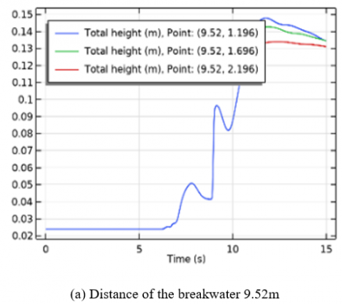
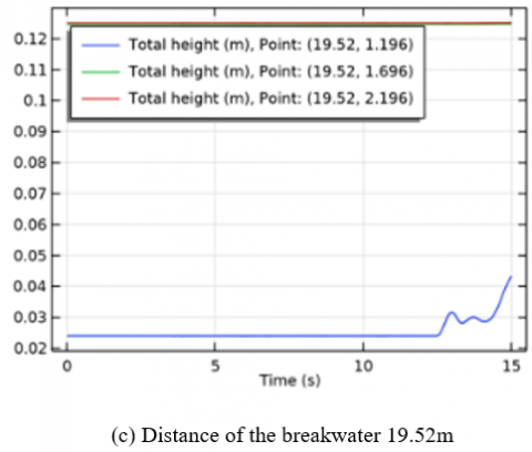
The stability of wave propagation is indicated by the amplitude distribution of sea water waves, given three critical points from the breakwater respectively 1.196m, 1.696m, and 2.196m for variations in the distance of the breakwater, namely 9.52m, 14.52m, and 19.52m. Simulation of wave amplitude distribution for variations in the position of the breakwater is shown in Figure 11.
Figure 11. Stability simulation with differences wave position
From the simulation results it is shown that the difference in the distance of the breakwater that is carried out will give a difference in the value of the amplitude distribution $(\lambda)$ for each position. The computations are carried out on an interval of 0<t<15 and show that a short distance will give a large amplitude, which means that the wave splitting does not work optimally because it gives such a large wave height value. Placement of the breakwater with a distance of 19.52m gives a low wave height, it can be seen that the wave amplitude starts to occur at t=10s the computation is done. The height of each wave is shown in Table 1.
Table 1. Amplitude magnitude to variety of position
|
$u(x, t)$ |
$h_b$=1.196 |
$h_b$=1.696 |
$h_b$=2.196 |
|
x=9.52 |
0.13439 |
0.13438 |
0.13097 |
|
x=14.52 |
0.13988 |
0.13859 |
0.13161 |
|
x=19.52 |
0.043203 |
0.12468 |
0.12515 |
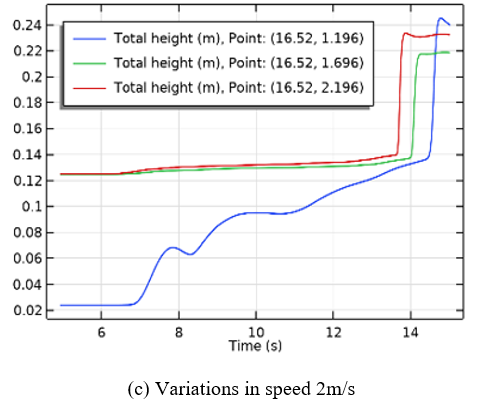
Figure 12. The difference between the change in the value of λ and the variation in the speed of the incident wave
Figure 12 represents the change in amplitude that occurs due to wave breaking based on variations in propagation speed. Waves that come at 2m/s have the biggest wave height, whereas waves at 1m/s have the lowest wave height. The simulation results of wave heights for speed variations are shown in Table 2.
Table 2. Amplitude magnitude to variety of position
|
$u(x, t)$ |
$h_b$=1.196 |
$h_b$=1.696 |
$h_b$=2.196 |
|
$u_t$=1 |
0.039990 |
0.12481 |
0.12538 |
|
$u_t$=1,5 |
0.090519 |
0.12726 |
0.12909 |
|
$u_t$=2 |
0.23979 |
0.21846 |
0.23229 |
Table 1 shows the magnitude of the wave height that occurs in the interval t(0, 15), which gives the result that for a breakwater that is 19.52m, it gives a large wave height on the surface that is equal to 0.12515m, which is the minimum wave height value from a variation of 9.52m, which is 0.13097m, and a distance of 14.52m produces a wave height of 0.13161m. To provide a difference in the computational results that have been obtained, computations will be carried out on variations in the speed of the incoming wave propagation with the assumption that the breakwater is positioned at=16.92m with variations in speed, namely 1m/s, 1.5m/s, and 2m/s. The simulation is shown in Figure 12.
Table 2 shows the magnitude of the wave height that occurs in the interval t(0, 15), which gives the result that the incoming wave with=1m/s gives a large wave height on the surface that is equal to 0.12538m, which is the minimum wave height value of the variation=1.5m/s of 0.12909m, and=2m/s produces a wave height of 0.23229m. The advantage of the results obtained can be seen that the distance between the breakwaters can affect the stability of sea waves with different wave speeds. This simulation makes it possible to identify and address potential problems or weaknesses in a design prior to implementation in the real-world. While simulation software such as COMSOL can provide an initial view of how a design will perform, validating the design through comparison with real-world data and results is essential. This helps ensure that the simulation model accurately represents the physical phenomena that occur in the field.
Based on the research that has been done, it can be concluded that the simulation of wave attenuation has a significant impact on the value of the wavelength, and the magnitude of the wave propagation velocity generated by the simulation time is 15 seconds with several simulation variations, namely variations in the placement of the breakwater at a distance of 10m, 15m, and 20m. the smaller the wave height and, consequently, the more stable the simulation of the component’s movement’s direction and speed on $[x, y, t]$ for each $\lambda_1=[20,2,15]$ is $0,12515 \mathrm{~m}, \lambda_2=$ $[15,2,15]$ is $0,13161 \mathrm{~m}$, and $\lambda_3=[10,2,15]$ is $0,13097 \mathrm{~m}$.
The study was funded by Research Institution of Universitas Sumatera Utara 2022 International Collaborative Research Scheme (Grant No.: 367/UN5.2.3.1/PPM/KP-TALENTA/2022).
[1] Winarta, B., Damarnegara, A.A.N.S., Anwar, N., Juwono, P.T. (2018). Analysis of Waikelo Port breakwater failure through 2D wave model. Civil and Environmental Science Journal, 1(2): 88-95. https://doi.org/10.21776/ub.civense.2018.00102.6
[2] Ghani, F.A.A., Ramli, M.S., Noar, N.A.Z.M., Kasim, A.R.M., Greenhow, M. (2017). Mathematical modelling of wave impact on floating breakwater. In Journal of Physics: Conference Series, IOP Publishing, 890(1): 012005. https://doi.org/10.1088/1742-6596/890/1/012005
[3] Peng, W., Huang, X.Y., Fan, Y.N., Zhang, J.S., Ren, X.Y. (2017). Numerical analysis and performance optimization of a submerged wave energy converting device based on the floating breakwater. Journal of Renewable and Sustainable Energy, 9(4): 044503. https://doi.org/10.1063/1.4997505
[4] Keuthen, M., Kraft, D. (2016). Shape optimization of a breakwater. Inverse Problems in Science and Engineering, 24(6): 936-956. https://doi.org/10.1080/17415977.2015.1077522
[5] Lin, M.Y., Li, C.Y., Wang, A.P. (2014). Particle based simulation for solitary waves passing over a submerged breakwater. Journal of Applied Mathematics and Physics, 2(6): 269-276. https://doi.org/10.4236/jamp.2014.26032
[6] Dentale, F., Donnarumma, G., Carratelli, E.P. (2014). Simulation of flow within armour blocks in a breakwater. Journal of Coastal Research, 30(3): 528-536. https://doi.org/10.2112/JCOASTRES-D-13-00035.1
[7] Zhang, N., Guo, K., Zhang, W.Z. (2012). Two-dimensional numerical wave simulation for port with submerged breakwater. Applied Mechanics and Materials, 226: 1343-1347. https://doi.org/10.4028/www.scientific.net/AMM.226-228.1343
[8] Wurm, J., Woittennek, F. (2022). Energy-based modeling and simulation of shallow water waves in a tube with moving boundary. IFAC-PapersOnLine, 55(20): 91-96. https://doi.org/10.1016/j.ifacol.2022.09.077
[9] Boschitsch, A.H., Fenley, M.O. (2004). Hybrid boundary element and finite difference method for solving the nonlinear Poisson Boltzmann equation. Journal of Computational Chemistry, 25(7): 935-955. https://doi.org/10.1002/jcc.20000
[10] Gusev, O.I., Khakimzyanov, G.S., Skiba, V.S., Chubarov, L.B. (2023). Shallow water modeling of wave-structure interaction over irregular bottom. Ocean Engineering, 267: 113284. https://doi.org/10.1016/j.oceaneng.2022.113284
[11] Marchesi, E., Negri, M., Malavasi, S. (2020). Development and analysis of a numerical model for a two-oscillating-body wave energy converter in shallow water. Ocean Engineering, 214: 107765. https://doi.org/10.1016/j.oceaneng.2020.107765
[12] Karmpadakis, I., Swan, C., Christou, M. (2022). A new wave height distribution for intermediate and shallow water depths. Coastal Engineering, 175: 104130. https://doi.org/10.1016/j.coastaleng.2022.104130
[13] Khater, M.M.A., Botmart, T. (2022). Unidirectional shallow water wave model; computational simulations. Results in Physics, 42: 106010. https://doi.org/10.1016/j.rinp.2022.106010
[14] Huang, S., Sheng, S.W., You, Y.G., Gerthoffert, A., Wang, W.S., Wang, Z.P. (2018). Numerical study of a novel flex mooring system of the floating wave energy converter in ultra-shallow water and experimental validation. Ocean Engineering, 151: 342-354. https://doi.org/10.1016/j.oceaneng.2018.01.017
[15] Chang, T.J., Yu, H.L., Wang, C.H., Chen, A.S. (2022). Dynamic-wave cellular automata framework for shallow water flow modeling. Journal of Hydrology, 613: 128449. https://doi.org/10.1016/j.jhydrol.2022.128449
[16] Kounadis, G., Dougalis, V.A. (2020). Galerkin finite element methods for the shallow water equations over variable bottom. Journal of Computational and Applied Mathematics, 373: 112315. https://doi.org/10.1016/j.cam.2019.06.031
[17] Zhang, Z.Q., Zhou, B.H., Li, X.B., Wang, Z. (2022). Second-order stokes wave-induced dynamic response and instantaneous liquefaction in a transversely isotropic and multilayered poroelastic seabed. Frontiers in Marine Science, 9: 1082337. https://doi.org/10.3389/fmars.2022.1082337
[18] Shojaeefard, M.H., Nourbakhsh, S.D., Zare, J. (2017). An investigation of the effects of geometry design on refrigerant flow mal-distribution in parallel flow condenser using a hybrid method of finite element approach and CFD simulation. Applied Thermal Engineering, 112: 431-449. https://doi.org/10.1016/j.applthermaleng.2016.10.009
[19] Kumar, P. (2021). Mathematical modeling of arbitrary shaped harbor with permeable and impermeable breakwaters using hybrid finite element method. Ocean Engineering, 221: 108551. https://doi.org/10.1016/j.oceaneng.2020.108551
[20] Busto, S., Dumbser, M., Río-Martín, L. (2021). Staggered semi-implicit hybrid finite volume/finite element schemes for turbulent and non-Newtonian flows. Mathematics, 9(22): 2972. https://doi.org/10.3390/math9222972
[21] Takahashi, Y., Wakao, S. (2008). Large‐scale magnetic field analysis by the hybrid finite element‐boundary element method combined with the fast multipole method. Electrical Engineering in Japan, 162(1): 73-80. https://doi.org/10.1002/eej.20508
[22] Jin, Y., Li, S., Ren, L. (2020). A new water wave optimization algorithm for satellite stability. Chaos, Solitons & Fractals, 138: 109793. https://doi.org/10.1016/j.chaos.2020.109793
[23] Cardinale, T., De Fazio, P., Grandizio, F. (2016). Numerical and experimental computation of airflow in a transport container. International Journal of Heat and Technology, 34(4): 734-742. https://doi.org/10.18280/ijht.340426
[24] Hachicha, I. (2014). Global existence for a damped wave equation and convergence towards a solution of the Navier-Stokes problem. Nonlinear Analysis: Theory, Methods & Applications, 96: 68-86. https://doi.org/10.1016/j.na.2013.10.020
[25] Li, Y.P. (2016). Vanishing viscosity and Debye-length limit to rarefaction wave with vacuum for the 1D bipolar Navier-Stokes-poisson equation. Zeitschrift für angewandte Mathematik und Physik, 67(3): 1-22. https://doi.org/10.1007/s00033-016-0637-z
[26] Liu, T.P., Noh, S.E. (2015). Wave propagation for the compressible Navier-Stokes equations. Journal of Hyperbolic Differential Equations, 12(2): 385-445. https://doi.org/10.1142/S0219891615500113
[27] Luo, T., Yin, H.Y., Zhu, C.J. (2018). Stability of the rarefaction wave for a coupled compressible Navier-Stokes/Allen-Cahn system. Mathematical Methods in the Applied Sciences, 41(12): 4724-4736. https://doi.org/10.1002/mma.4925
[28] Marpaung, T.J., Tulus, Suriati, Siringoringo, Y.B., Syahputra, M.R. (2019). Heat transfer simulation on window glass using COMSOL multiphysic. In Journal of Physics: Conference Series, IOP Publishing, 1235(1): 012065. https://doi.org/10.1088/1742-6596/1235/1/012065
[29] Khairani, C., Tulus, Suriati, Marpaung, T.J. (2019). Computational analysis of fluid behaviour around airfoil with Navier-Stokes equation. In Journal of Physics: Conference Series, IOP Publishing, 1376(1): 012003. https://doi.org/10.1088/1742-6596/1376/1/012003
[30] Sitompul, O.S., Tulus, Mardiningsih, Sawaluddin, Ihsan, A.K.A.M. (2018). Shear rate analysis of water dynamic in the continuous stirred tank. In IOP Conference Series: Materials Science and Engineering, IOP Publishing, 308(1): 012048. https://doi.org/10.1088/1757-899X/308/1/012048
[31] Chaudhury, P., Samantary, S. (2019). Finite element modelling of EDM of aluminium particulate metal matrix composites considering temperature dependent properties. Revue des Composites et des Materiaux Avances, 29(1): 53-62. https://doi.org/10.18280/rcma.290109
[32] Shojaeefard, M.H., Nourbakhsh, S.D., Zare, J. (2017). An investigation of the effects of geometry design on refrigerant flow mal-distribution in parallel flow condenser using a hybrid method of finite element approach and CFD simulation. Applied Thermal Engineering, 112: 431-449. https://doi.org/10.1016/j.applthermaleng.2016.10.009
[33] Kumar, P. (2018). Modeling of shallow water waves with variable bathymetry in an irregular domain by using hybrid finite element method. Ocean Engineering, 165: 386-398. https://doi.org/10.1016/j.oceaneng.2018.07.024