Bashar E.A. Badr*![]() | Ibrahim Altawil
| Ibrahim Altawil![]() | Mohammed Almomani
| Mohammed Almomani![]() | Mohammed Al-Saadi | Mohammad Alkhurainej
| Mohammed Al-Saadi | Mohammad Alkhurainej
© 2023 IIETA. This article is published by IIETA and is licensed under the CC BY 4.0 license (http://creativecommons.org/licenses/by/4.0/).
OPEN ACCESS
The challenges associated with diagnosing faults in three-phase induction motors necessitate the development of innovative, non-invasive methods that can increase efficiency and reduce costs. This study presents a novel approach to fault detection in these motors, leveraging advanced machine learning technology. The primary focus is the identification of faults related to the stator, including single-phase and three-phase faults, current interruptions, and sudden torque changes. Convolutional Neural Networks (CNN), inspired by the human visual nervous system, form the backbone of the proposed fault detection methodology. This technique utilizes external measurements for processing, circumventing the need for intrusive measures such as opening the motor or installing internal sensors. The non-intrusive nature of this method not only simplifies the process but also significantly reduces associated costs. The CNN-based approach offers superior accuracy in diagnosing faults, facilitating timely prevention measures and potentially saving human lives. It also reduces the time and effort required to identify fault types, thus minimizing motor downtime and associated costs. Simulations were conducted using MATLAB software, and individual fault scenarios were applied and analyzed. The results obtained demonstrate the efficacy of the CNN-based fault diagnosis method, thereby highlighting its potential for implementation in real-world scenarios. This study contributes to the field by providing a detailed exploration of a non-invasive, cost-effective, and highly accurate method for fault detection in three-phase induction motors. It opens avenues for further research into the application of machine learning techniques for fault diagnosis in other types of motors.
three-phase induction motor, deep learning, artificial intelligence, fault diagnosis, wavelet signal processing, conventional neural network, google net algorithm, convolutional neural networks
Three-phase induction motors are integral to numerous industrial applications, including wood-cutting machines, blowers, pumps, elevators, lifters, compressors, and critical processes in mining, machinery, and chemical industries. Their popularity stems from their simple construction, high initial torque, robust speed regulation, and respectable overload capacity. However, these motors are not exempt from operational failings, such as motor winding burnouts, making it essential to detect any anomalies that could compromise motor health.
Rather than resorting to replacement, it is more advantageous to identify the root causes of the windings' damage in three-phase motors. A broad spectrum of failure situations warrants observation, including single-phase burnout, overload, voltage imbalance, and voltage spikes common in motors controlled by variable frequency drives. Typical winding problems in three-phase motors range from shorted turns, winding shorted to frame, phase-to-phase short, open winding, to burned windings resulting from single-phase operation, submerged motors, and various rotor issues such as open rotor bars, open end rings, misalignment of rotor/stator iron, rotor dragging on the stator, and rotor looseness on the shaft. Notably, bearing failures account for nearly 40% of all faults.
In recent years, a myriad of techniques has emerged for diagnosing faults in three-phase induction motors. These range from simple to complex methodologies, as elaborated in the related work section. Among the most potent tools for this purpose are Deep Learning (DL) and Convolutional Neural Network (CNN) techniques, frequently used in audio and visual recognition and classification, amongst other civilian applications. CNNs, with their capacity for autonomous spatial feature learning from raw data, have delivered state-of-the-art performance in image classification and recognition.
This study implements a CNN-based method to diagnose five different types of faults in three-phase induction motors. It facilitates various analyses on these motors under conditions including normal operation (NR), phase interruption (PI), sudden change in torque (CT), single-phase fault (SPF), and three-phase fault (TPF). Deep learning stands as a compelling technique for fault diagnosis in three-phase induction motors. This cutting-edge approach can interpret signals from the machine non-intrusively and diagnose the aforementioned faults accurately, thereby saving costs, preserving the machine, and potentially even saving lives.
Various fault detection and identification techniques hinge on the analysis of the stator current's spectral signature. One such technique utilizes the power spectrum of the stator current for identifying broken rotor bar faults, achieved through the Fast Fourier Transform of the current signal [1, 2]. Another renowned approach engages the negative sequence components of the stator current to detect inter-turn short circuits [3, 4]. This method identifies asymmetries generated by a faulty motor with shorted turns in the stator winding, which induces a negative sequence current that can pinpoint the fault. The negative sequence is derived through a vector interpretation of unbalanced three-phase currents or voltages [5]. However, certain factors such as unbalanced power supply voltage, specific types of loads, and instrument errors can engender negative sequence currents even in healthy motors, leading to potential misclassification. Although some studies have considered these effects, the technique remains incapable of detecting faults in induction motors with inherently unbalanced windings, as illustrated in the study [6].
In their research, Yao et al. [7] employed a distinctive technique known as Acoustic-Based Diagnosis (ABD). This method, designed to diagnose gear faults, leverages a multi-scale convolutional learning structure and attention mechanism. The necessity for this approach stemmed from the challenge of distinguishing between normal and faulty signals during gear fault diagnosis, as the process largely relies on vibration signals.
Ngaopitakkul et al. [8] introduced a decision algorithm in another study. This algorithm utilizes an Artificial Neural Network (ANN) to diagnose faults in single-line transmission lines, employing the Discrete Wavelet Transform (DWT) and Backpropagation Neural Networks.
Ge et al. [9] resorted to Complete Ensemble Empirical Mode Decomposition (CEEMD) for extracting bearing fault features, while diagnosis was achieved by injecting adaptive noise and amplifying the mode characteristic of the rotational machines.
Deng et al. [10] explored bearing fault diagnosis in rotational machines using a method centered on opacity correlation classification and an empirical wavelet transform sub-modal hypothesis test. A comparison between ANN and CNN in fault diagnosis was conducted [11], revealing that CNN outperformed ANN in fault detection, particularly in environments with static motor surroundings. Additionally, CNN boasts a simpler structure and a shorter learning curve compared to ANN.
Han et al. [12] employed a fusion of three techniques for the real-time fault diagnosis of induction machines, involving ANN, DWT, feature extraction, and a genetic algorithm (GA).
Heydarzadeh et al. [13] used Deep Neural Networks (DNN) to detect gear faults by feeding three monitoring signals (vibration, acoustic, and torque) extracted from the discrete wavelet domain to precisely diagnose five types of faults. This study demonstrated that DNN outperforms traditional processing methods due to its deep data-driven approach, requiring minimal prior knowledge for feature extraction and not necessitating any specific requirements for monitoring signals.
Shao et al. [14] developed a deep learning approach based on Deep Belief Networks (DBN) to learn features from the frequency distribution of vibration signals and characterize the working status of induction motors. This method amalgamated feature extraction procedures with classification tasks to achieve automated and intelligent fault diagnosis. The DBN model, constructed by stacking multiple units of a Restricted Boltzmann Machine (RBM), was trained using a layer-by-layer pre-training algorithm. This technique demonstrated superior results compared to previous methods. The obtained simulated results provide a close approximation to actual faults.
3.1 Deep learning usage in fault diagnosis
Deep Learning (DL) harnesses feature characterization-based techniques such as Recurrent Neural Networks (RNNs), Deep Neural Networks (DNNs), and Convolutional Neural Networks (CNNs) to tackle the intricacy of feature engineering by directly extracting feature descriptors from raw signals. Among these techniques, CNNs have shown exceptional efficacy in learning synthesized features from raw signals or images [15]. DL finds extensive applications in a wide array of fields, including computer vision, machine vision, and natural language processing.
3.2 Artificial neural networks (NNs)
In an effort to enhance the efficiency of induction machines and extend their lifespan commensurate with productivity growth, experts are fervently developing novel techniques to assist in fault monitoring, detection, and diagnosis [16]. Many of these Deep Learning (DL) approaches analyze vibration and stator current, given their ease and reliability of measurement [5]. Leveraging Neural Networks (NNs), Artificial Intelligence techniques are developed to detect faults in induction motors and furnish information regarding the root cause of the failure [17-21]. The DL approach is easily implemented by capturing process information from measurements and using it to train neural networks [22]. This method offers a significant advantage in generating straightforward information on fault characteristics, such as type and size, without the need for complex mathematical models.
3.3 Fault classification using neural network
Figure 1. Fault detection procedure
The fault diagnosis process can be represented by Figure 1, which consists of four steps: data collection, feature extraction, feature selection, and fault classification. In Figure 1, NR is the normal case, PI is phase interrupt, TPF is a three-phase fault and SPF is a single-phase fault.
3.4 Data collection and acquisition
To ensure accuracy in the diagnosis, multiple samples must be taken. These samples are obtained by measuring specific parameters such as stator current or rotor current. Typically, experts conduct experiments by using specialized tools to measure the stator current under various fault conditions, which are then compared. However, to obtain a meaningful diagnosis, a large number of samples - often exceeding 200 - may be required.
3.5 Feature extraction
Statistical parameter-based feature extraction is a technique used to identify faults and their types. It involves calculating 13 parameters of the statistical samples for the current, which are then used as input data. The minimum group of the statistical sample analyzed comprises the standard deviation, maximum and minimum values of skewness and kurtosis coefficients [23]. Pearson’s coefficient of skewness can be given by Eq. (1).
$g_2=\frac{3(\bar{x}-\tilde{x})}{S_x}$ (1)
where, $\bar{x}$ is the mean square value and $\tilde{x}$ is the average value. $S_x$ is the standard deviation of the samples. Whereas the sample coefficient of variation is $V_x$ given by Eq. (2).
$V_x=\frac{S_x}{\bar{x}}$ (2)
Eq. (3) illustrates the moments of the sample around the mean value of the sample's set.
$m_r=\frac{\sum_{i=1}^n\left(x_i-\tilde{x}\right)^r}{n}$ (3)
when r=2, the calculation of m2 reflects how the sample is spread around its center, while m3 indicates the degree to which the samples are clustered around the center. Typically, the second, third, and fourth moments are used to measure the coefficient of skewness in a sample, with g3 and g4 representing the skewness and kurtosis coefficients, respectively, as given by Eqs. (4)-(5). The covariance between two dimensions of a particular sample can be calculated by Eq. (6) [23]:
$g_3=\frac{m_3}{\left(\sqrt{m_2}\right)^3}$ (4)
$g_4=\frac{m_4}{\left(\sqrt{m_2}\right)^4}$ (5)
$C_{j k}=\frac{\sum_{i=1}^n\left(x_{i j}-\overline{x_j}\right)\left(x_{i k}-\overline{x_k}\right)}{(n-1)}$ (6)
3.6 Feature selection
At this stage, it is crucial to select the most informative feature from the feature set to improve the classifier's performance and prevent errors during the selection process by disregarding irrelevant or excessive features [23]. The optimal feature can be selected from the primary feature set by applying the Principal Component Analysis (PCA) technique, which linearly or non-linearly converts the primary feature set into a smaller set, making it easier to handle and comprehend than the large set. This technique is commonly used as a conventional method of multivariable statistical analysis to extract the optimal features and decrease the gap between the original features [23].
3.7 Feature classification
A neural network can be utilized to classify features by using the time domain vibration of the three-phase dimension and three-phase current as inputs, which allows for fault detection. This NN consists of input, output, and hidden layers that convert the input data into a format that is useful for the output layer. To regulate the hidden layers of neurons when the network's results are unsatisfactory, the posterior diffusion technique can be employed in NN. Figure 2 illustrates the different layers of the artificial neural network, with the three orange circles indicating the input layers and the red circles representing the output layers. The four blue and four green circles denote the hidden layers, and all of them contain active nodes [24].
Figure 2. Artificial neural network
In an artificial neural network, each node is linked to the node of the subsequent layer, and every connection possesses a particular weight, representing the influence of the node on the subsequent layer node. By increasing the weight, the range of information reflection from one node to the next can be expanded. If the orange node's value is multiplied by its corresponding weight, and the resulting values are added, the blue node's value will be obtained. This blue node is then defined as an activation function that determines whether the node is activated and how active it will be, based on the summarized value [24].
3.8 Convolutional neural network
The most frequently used form of deep learning, the convolutional neural network (CNN), derives its name from the mathematical process of convolution performed between matrices [25]. While CNNs are built upon artificial neural networks (ANNs) that seek to replicate the workings of the human brain, they feature distinct layers including the convolutional and fully connected layers, which contain parameters, and non-parameter layers like the non-linearity and pooling layers [26, 27].
3.9 Convolution neural network construction
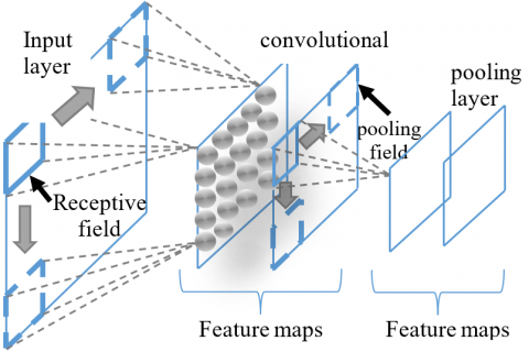
As shown in Figure 3, the CNN architecture is divided into two main parts. The first part comprises the input layer, the convolutional layer, and the pooling layer, which work sequentially to extract features from the input. The second part is responsible for feature classification and includes the fully-connected layer and output layer. After the final pooling layer, the extracted features are passed to the fully connected layer, which then performs the classification task [24, 27].
Figure 3. Structure of CNN
In the classification process, the input data is passed from the input layer to the convolutional layer to identify local features, which are then stored in a feature map [28]. As shown in Figure 3, the input layer and convolutional layer are connected through a receptive field, which is a small square matrix of weights that is applied to a specific input area. The feature map consists of nodes, with each node connected to a specific input area determined by the receptive field. This field moves across the input section over both horizontal and vertical axes, performing a convolution operation to identify features [29].
3.10 Wavelet transform
Wavelet transformation methods have become increasingly popular in the field of fault detection due to their ability to extract information about a feature in both the frequency and time domains, making them highly efficient. Additionally, wavelet techniques have been shown to be more effective in fault diagnosis compared to other methods like the Fourier transform, which requires the use of a single function to make a linear decision across the entire frequency domain, unlike the wavelet transform method [30, 31]. There are several types of wavelet transformation methods, but the most significant ones include the discrete wavelet transform (DWT), which is represented by Eq. (7), and the continuous wavelet transform (CWT), which is represented by Eq. (8). The CWT is further divided into real wavelets and complex wavelets [32, 33].
$D W T(m . k)=\frac{1}{\sqrt{a_0^m}} \sum x(n) g\left(\frac{k-n b_0 a_0^m}{a_0^m}\right)$ (7)
$C W T(m . N)=\int_{-\infty}^{\infty} f(t) \psi_{m . n}^*(t)$ (8)
$\psi_{m . n}(t)=2^{-1 / 2} \psi\left(2^{-m} t-n\right)$ (9)
$C W T_{a . b}(t)=|a|^{-1 / 2} \psi\left(\frac{t-b}{a}\right)$ (10)
The input signal x is analyzed using the fundamental wavelet g, with scaling and translation parameters a and b, respectively. The conjugate wavelet function $\psi_{m . n}^*$, represented by Eq. (9), is used when a=b=2, indicating that this equation is only valid for the perpendicular base of the wavelet transform; otherwise, Eq. (10) is used [30]. The waveform signal f(t) is used, with parameters m and n, to convert the original signal into a new signal with a smaller scale that matches the high-frequency components.
Discrete wavelet transformation is a preferable option for digital computers, as it provides an alternative solution to the resolution problem [31]. The properties of wavelet transformation can be summarized in two main points [30-32]:
1. The fact that if the wavelet satisfies the condition defined by Eq. (11), a signal with finite power can be reconstructed without requiring all of its analysis values [30].
$\frac{|\psi(\omega)|^2}{|\omega|} d \omega<+\infty$ (11)
where, ψ(ω) is the Fourier transform function of the wavelet transformation function ψ(t) that is used to examine signals and remodel them without mislaying any data.
2. To handle the quadratic relationship between the time scale generated by the wavelet transform and the input signal, certain regularity conditions are enforced to ensure the smoothness and compactness of the wavelet function in both time and frequency domains [30].
The analysis can be carried out by filtering and selecting samples, and can also be performed with a sequential approach [34]. However, the total number of analysis levels (L) can be calculated using the following formula:
$L \geq \frac{\log \left(f_s / f\right)}{\log (2)}+1$ (12)
Eq. (12) can be used to calculate the total number of analysis levels (L) in wavelet transformation, based on the sample frequency (fs) and the fundamental frequency (f) of the input signal. However, these levels cannot be altered unless new data with a different sampling frequency is acquired, which can pose a challenge for fault diagnosis in time-varying conditions [35]. For instance, using the values fs=1KHz and f=50Hz, Eq. (12) would yield six analysis levels for each wavelet waveform, as shown in Table 1 [30].
Table 1. Frequency bands for six levels of wavelet signals
|
Approximation ai |
Frequency Chains Hz |
Details di |
Frequency Chains Hz |
|
a6 |
[0-16.125] |
d6 |
[16.125-32.250] |
|
a5 |
[0-32.250] |
d5 |
[32.250-64.500] |
|
a4 |
[0-64.500] |
d4 |
[64.500-125.00] |
|
a3 |
[0-125.00] |
d3 |
[125.00-250.00] |
|
a2 |
[0-250.00] |
d2 |
[250.00-500.00] |
|
a1 |
[0-500.00] |
d1 |
[500.00-1000.0] |
Eq. (13) demonstrates how the desired data can be analyzed using a wavelet signal, taking into account both the sampling frequency fs and the resolution R [30].
$D_{\text {desired }}=f_s / R$ (13)
Figure 4. Simulation of three-phase induction motor system using MATLAB
Figure 4 shows a Simulink model created using MATLAB software, which includes running code to compare five categories of three-phase induction motors (IMs). Each category has its Simulink model and code, with 100 data points for each category. The resulting RMS current is displayed both as a curve and an image, enabling the operator to understand and evaluate the situation. These input data are then used in the deep learning process, which includes a code for classification of the categories. In addition to the previously obtained results, the training process and confusion matrix provide an overview of the five scenarios.
Table 2. Three-phase squirrel cage induction motor parameters
|
No. |
Parameters |
Value |
|
1 |
P |
5 hp |
|
2 |
V |
460 V |
|
3 |
f |
60 Hz |
|
4 |
Rs |
1.115 ohm |
|
5 |
$R_r{ }^{\prime}$ |
1.083 ohm |
|
6 |
Ls |
0.005974 H |
|
7 |
Lr |
0.005974 H |
|
8 |
Lm |
0.203700 H |
The system depicted in Figure 4 uses a three-phase squirrel cage induction motor with parameters shown in Table 2. A LC filter is utilized in this study to smooth the output current of the inverter, which is used to build a control circuit to regulate the motor's speed. The voltage frequency control (V/F) technique is employed, as shown in Figure 5, which maintains a constant motor flux by achieving the ratio of output voltage to the frequency, thus preventing weak magnetic and magnetic saturation phenomena from occurring [36, 37]. Additionally, Pulse-Width Modulation (PWM), as depicted in Figure 6, is used in the Simulink to reduce the average power delivered by an electrical signal by chopping it up into discrete parts. The motor speed and torque in the system were calibrated to be 150 rpm and 10 N.m, respectively, and a PI-controller is used to perfectly regulate the motor's speed.
Figure 5. Current curve in NR-Category
This research covers five categories: normal operation (NR), where the induction motor operates without any abnormal actions; change torque (CT), where the IM is operated with random values of torque; phase interrupts (PI) [38], where an outage action occurs at one of the phases on IM; single phase fault (SPF), where a phase-to-ground fault occurs in IM; and three-phase fault (TPF), which is the worst-case scenario.
4.1 Generating data
The first step in creating a simulation model and code is generating data for each fault category. This can be accomplished by adding various modifications to each data, such as varying the duration or starting time of the fault. This process will generate 100 samples for each of the five scenarios, resulting in a total of 500 samples that can be used for the deep learning and training-testing processes. These samples will be stored and used for later analysis.
Case 1: Normal operation
The current output waveform of a three-phase induction motor during normal operation can be observed in Figure 5 in the time domain. As depicted in the diagram, the motor initially operates with a starting RMS current of 22 A for the first 0.3 seconds. After that, at 0.5 seconds, the motor runs with a rated RMS current of 4 A.
Figure 6 represents a wavelet transformation image of the RMS current waveform displayed in Figure 4, depicting a 2D-Continuous Wavelet Transform in the time-frequency domain. In the "NR" category of the diagram, the blue region shown in Figure 5, which extends from 0.5 seconds, indicates that the current remained within normal limits, and the system operated at the fundamental frequency of 50 Hz. However, the yellow region, which appears in the figure during the first 0.3 seconds, signifies that the RMS current value was higher compared to the rated current.
Figure 6. Wavelet image for the current in NR-Category
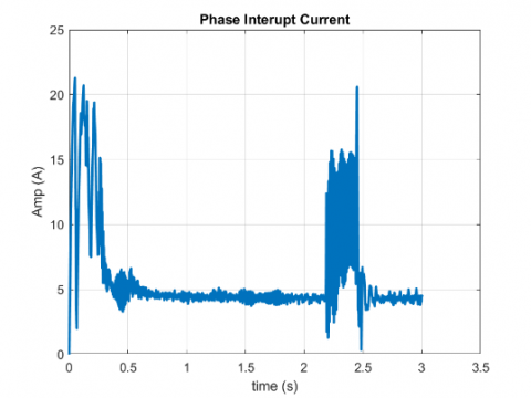
Case 2: Phase interrupt
In a three-phase IM, when an action occurs in one of the phases, a significant increase in current will occur during operation, as shown in Figure 7. In this figure, the waveform of the RMS current displays an abnormal current value, equivalent to 5 times the rated current, during the interval [2.2-2.5] seconds. Additionally, Figure 8 illustrates the wavelet form of the output current, where the yellow zones indicate that the output current has an abnormal value during the operation at the intervals [0-0.2] (starting current) and [2.2-2.5] (when one of the motor's phases is interrupted).
Figure 7. Current curve in PI-Category
Figure 8. Wavelet image for the current in PI-Category
Case 3: Sudden change torque
Figure 9 demonstrates the RMS current curve when the torque value suddenly changes due to a modification in rotor speed. The curve indicates two points with abnormal current values: the first region within the time interval [0-0.2] seconds, which is the starting current. The output current value gradually decreases until it reaches the rated current, followed by an instantaneous and abrupt rise in current value due to a sudden change in induced torque after one second of operation [39].
Figure 9. Current curve in CT-Category
Referring to the wavelet transformation image presented in Figure 10 for implementing the PI category, it is observed that the blue region is not entirely pure after 0.5 seconds of operation. In the first second, an abnormal action is visible, indicating a sudden change in current due to a modification in torque.
Figure 10. Wavelet image for the current in CT-Category
Case 4: Single-phase fault
A single phase to ground fault is one of the most common faults that occur in a three-phase IM. The current waveform resulting from this fault is illustrated in Figure 11, which shows the magnitude of the current and the duration of time when the fault occurred. On the other hand, Figure 12 presents the reflection image of this type of fault, where the yellow region between the time interval of 1 second and 2 seconds indicates the occurrence of a fault in that region with a frequency of 200 Hz.
Figure 11. Current curve in SPF-Category
Figure 12. Wavelet image for the current in SPF-Category
Case 5: Three-phase fault
Figure 13. Current curve in TPF-Category
Figure 13 illustrates a three-phase fault, which is the most perilous fault that may occur in an IM. It is crucial to prevent this type of fault from happening. However, the figure indicates an anomalous action taking place between [2.3-2.7] seconds with an RMS value around 20 times higher than the rated current, which is an extremely high value. If the appropriate action is not taken swiftly to prevent it, this dangerous alert could potentially harm the machine. In the wavelet image presented in Figure 14, it is evident that the yellow region has an exceptionally high and abnormal frequency value, approximately 1000 Hz, alerting the operator to the presence of a very high current in that time interval.
Figure 14. Wavelet image for the current in TPF-Category
4.2 Fault analysis using deep learning process
The second approach utilized in this research involves employing deep learning for fault classification using the neural network (NN) method. This method assists the operator in diagnosing the type of fault that may occur in the IM motor, enabling them to take appropriate actions to resolve it and maintain the motor's default lifespan. The running of the deep learning code results in two crucial processes: the training process and the testing process.
The simulation model of the deep learning process used specific parameters as shown in Table 3.
Table 3. Deep learning parameters
|
Algorithm Network Used |
Googlenet |
|
Weight Learn Rate Factor |
6 |
|
Batch Size |
30 |
|
Epoch Size |
10 |
|
Validation Frequency |
10 |
|
Execution Environment |
GPU |
|
Training Data |
70% |
|
Validation Data |
30% |
4.2.1 Training- process and testing stage
The success of the machine learning process relies heavily on the training and testing processes, which provide valuable data for operators to make informed decisions during the fault diagnosis process. During the training process, the system strives to achieve 100% accuracy to identify the type of fault, while the testing process indicates any errors or shortcomings in the system's fault specification. In this study, the simulation model discussed in section 4.1 generated a database that was utilized for the deep learning process of the training and testing processes. If there is a strong correlation between the features and labels, the database can be divided equally between the training and testing processes, but if there are concerns about the system's success, the proportion of data used for the training process can be increased. The research in question utilized 500 sampling data, with 100 samples from each category, and allocated 70% of the data for the training process and 30% for the testing process.
Figure 15. Training and testing process
Figure 15 depicts the process of training and testing a system to identify different types of faults. The first curve of the figure represents the accuracy of the system during the training process, and the highest accuracy achieved in the study was 98.67%, which is a very good result. This level of accuracy was obtained in a time of 57 seconds. On the other hand, the first curve of the figure also shows the testing process, which represents the validation of the system's ability to identify faults. In this case, the best validation result in the study was achieved at a frequency of 10 Hz. The figure also includes a second curve that shows the loss of the system in diagnosing faults. The system aims to minimize the loss to demonstrate its efficiency, and in this study, the value of the loss was 0.1, which is considered satisfactory.
4.2.2 Confusion matrix
Figure 16. Confusion matrix
During the training and testing process, a confusion matrix was created to assess the accuracy and loss of the system in determining the type of fault in each category and for the entire process. The confusion matrix is a two-dimensional table that shows the target class and output class to evaluate the performance of the deep learning algorithm. Figure 16 displays the confusion matrix that was generated during the training and testing process, consisting of 5 rows and 5 columns, with each row representing the actual class (output class) and each column representing the predicted class (target class). The diagonal of the confusion matrix indicates the number of input images that the system correctly identified and the number of input images that the system failed to distinguish.
The confusion matrix, as shown in Figure 16, indicates that the system was able to differentiate between four categories with 100% accuracy and 0.0% loss. However, the system encountered difficulty in identifying the 30 images in the SPF category. Of these 30 images, the system correctly identified 28 as SPF, but misclassified 2 as TPF, resulting in an accuracy of 93.3% and a loss percentage of 6.7% for this category. Overall, the system achieved an accuracy of 98.7% and a percentage error of 1.3%.
This study entailed the development of five simulation models, each accompanied by five unique codes executing different operational actions. Each running code generates 100 data points, culminating in 500 samples that serve as input for a deep learning model. This model predicts the type of fault and enables operators to take the appropriate preventative measures. The fault diagnosis process is two-fold: it generates data from five distinct categories and feeds them into the deep learning algorithm to differentiate between fault types. The system also trains and processes data to align with the label of the targeted class.
The results showcased a commendable accuracy rate of 98.7% and a training process time of just 57 seconds for fault detection, underscoring the efficiency and predominance of deep learning in contemporary technology. The algorithm operates effectively on a cost-effective embedded processing system, making it ideal for real-time monitoring in industrial contexts.
Utilizing deep learning theory in fault diagnosis offers two key advantages: It requires minimal prior knowledge for feature extraction and is insensitive to varying conditions, thus eliminating the need for specific presumptions or signal measurements.
|
CWT |
Continuous wavelet transform |
|
$D_{\text {desired }}$ |
Desired data |
|
DWT |
Discrete wavelet transform |
|
f |
fundamental frequency |
|
fs |
Sample frequency |
|
g |
Pearson’s coefficient of skewness |
|
L |
Total number of analysis levels |
|
R |
Resolution |
|
Sx |
Standard deviation |
|
Vx |
Sample coefficient of variation |
|
$\tilde{x}$ |
Average value |
|
$\bar{x}$ |
Mean square value |
|
Greek symbols |
|
|
$\psi_{m . n}^*$ |
Conjugate wavelet function |
|
$\psi_{m . n}$ |
Wavelet function |
|
$\psi(\omega)$ |
Fourier transform function |
|
$\psi(t)$ |
Wavelet transformation function |
[1] Benbouzid, M.E.H. (2000). A review of induction motors signature analysis as a medium for faults detection. IEEE Transactions on Industrial Electronics, 47(5): 984-993. https://doi.org/10.1109/41.873206
[2] Kliman, G.B., Koegl, R.A., Stein, J., Endicott, R.D., Madden, A.M. (1988). Noninvasive detection of broken rotor bars in operating induction motors. IEEE Transactions on Energy Conversion, 3(4): 873-879. https://doi.org/10.1109/60.9364
[3] Petruzella, F. (2016). Electric Motors and Control Systems. 1st ed. New York: Mcgraw-Hill Education.
[4] Hafezi, H., Jalilian, A. (2006). Design and construction of induction motor thermal monitoring system. In Proceedings of the 41st International Universities Power Engineering Conference, pp. 674-678. https://doi.org/10.1109/upec.2006.367564
[5] Thomson, W.T., Rankin, D., Dorrell, A.D. (1999). On-line current monitoring to diagnose airgap eccentricity in large three-phase induction motors-industrial case histories verify the predictions. IEEE Transactions on Energy Conversion, 14(4): 1372-1378. https://doi.org/10.1109/60.815075
[6] Kunihiro, N., Todaka, T., Enokizono, M. (2010). Loss evaluation of an induction motor model core by vector magnetic characteristic analysis. IEEE Transactions on Magnetics, 47(5): 1098-1101. https://doi.org/10.1109/tmag.2010.2072910
[7] Yao, Y., Zhang, S., Yang, S., Gui, G. (2020). Learning attention representation with a multi-scale CNN for gear fault diagnosis under different working conditions. Sensors, 20(4): 1233. https://doi.org/10.3390/s20041233
[8] Ngaopitakkul, A., Bunjongjit, S. (2013). An application of a discrete wavelet transform and a back-propagation neural network algorithm for fault diagnosis on single-circuit transmission line. International Journal of Systems Science, 44(9): 1745-1761. https://doi.org/10.1080/00207721.2012.670290
[9] Ge, M., Wang, J., Xu, Y., Zhang, F., Bai, K., Ren, X. (2018). Rolling bearing fault diagnosis based on EWT Sub-modal Hypothesis test and ambiguity correlation classification. Symmetry, 10(12): 730. https://doi.org/10.3390/sym10120730
[10] Deng, W., Zhao, H., Yang, X., Dong, C. (2017). A fault feature extraction method for motor bearing and transmission analysis. Symmetry, 9(5): 60. https://doi.org/10.3390/sym9050060
[11] Choi, D.J., Han, J.H., Park, S.U., Hong, S.K. (2020). Comparative study of CNN and RNN for motor fault diagnosis using deep learning. In 2020 IEEE 7th International Conference on Industrial Engineering and Applications (ICIEA), pp. 693-696. https://doi.org/10.1109/iciea49774.2020.9102072
[12] Han, T., Yang, B.S., Choi, W.H., Kim, J.S. (2006). Fault diagnosis system of induction motors based on neural network and genetic algorithm using stator current signals. International Journal of Rotating Machinery. https://doi.org/10.1155/ijrm/2006/61690.
[13] Heydarzadeh, M., Kia, S.H., Nourani, M., Henao, H., Capolino, G.A. (2016). Gear fault diagnosis using discrete wavelet transform and deep neural networks. In IECON 2016-42nd Annual Conference of the IEEE Industrial Electronics Society, pp. 1494-1500. https://doi.org/10.1109/iecon.2016.7793549
[14] Shao, S.Y., Sun, W.J., Yan, R.Q., Wang, P., Gao, R.X. (2017). A deep learning approach for fault diagnosis of induction motors in manufacturing. Chinese Journal of Mechanical Engineering, 30(6): 1347-1356. https://doi.org/10.1007/s10033-017-0189-y
[15] Hammo, R. (2014). Faults identification in three-phase induction motors using support vector machine. Master’s Thesis. Bowling Green State University.
[16] Albawi, S., Mohammed, T.A., Al-Zawi, S. (2017). Understanding of a convolutional neural network. In 2017 International Conference on Engineering and Technology (ICET), pp. 1-6. https://doi.org/10.1109/icengtechnol.2017.8308186
[17] Akin, B., Orguner, U., Toliyat, H.A., Rayner, M. (2008). Low order PWM inverter harmonics contributions to the inverter-fed induction machine fault diagnosis. IEEE Transactions on Industrial Electronics, 55(2): 610-619. https://doi.org/10.1109/tie.2007.911954
[18] Faiz, J., Ebrahimi, B.M., Akin, B., Toliyat, H.A. (2007). Finite-element transient analysis of induction motors under mixed eccentricity fault. IEEE Transactions on Magnetics, 44(1): 66-74. https://doi.org/10.1109/tmag.2007.908479
[19] Ballal, M.S., Khan, Z.J., Suryawanshi, H.M., Sonolikar, R.L. (2007). Adaptive neural fuzzy inference system for the detection of inter-turn insulation and bearing wear faults in induction motor. IEEE Transactions on Industrial Electronics, 54(1): 250-258. https://doi.org/10.1109/tie.2006.888789
[20] Yang, B.S., Oh, M.S., Tan, A.C.C. (2009). Fault diagnosis of induction motor based on decision trees and adaptive neuro-fuzzy inference. Expert Systems with Applications, 36(2): 1840-1849. https://doi.org/10.1016/j.eswa.2007.12.010
[21] Zidani, F., Diallo, D., Benbouzid, M.E.H., Naït-Saïd, R. (2008). A fuzzy-based approach for the diagnosis of fault modes in a voltage-fed PWM inverter induction motor drive. IEEE Transactions on Industrial Electronics, 55(2): 586-593. https://doi.org/10.1109/iemdc.2005.195806
[22] Cusidócusido, J., Romeral, L., Ortega, J.A., Rosero, J.A., Espinosa, A.G. (2008). Fault detection in induction machines using power spectral density in wavelet decomposition. IEEE Transactions on Industrial Electronics, 55(2): 633-643. https://doi.org/10.1109/pesc.2006.1712271
[23] Bai, T., Yang, J., Duan, L., Wang, Y. (2020). Fault diagnosis method research of mechanical equipment based on sensor correlation analysis and deep learning. Shock and Vibration, 1-11. https://doi.org/10.1155/2020/8898944
[24] Ghate, V.N., Dudul, S.V. (2009). Fault diagnosis of three phase induction motor using neural network techniques. In 2009 Second International Conference on Emerging Trends in Engineering & Technology, pp. 922-928. https://doi.org/10.1109/icetet.2009.100
[25] Chattopadhyay, P., Saha, N., Delpha, C., Sil, J. (2018). Deep learning in fault diagnosis of induction motor drives. In 2018 Prognostics and System Health Management Conference (PHM-Chongqing), pp. 1068-1073. https://doi.org/10.1109/phm-chongqing.2018.00189
[26] Ramachandran, R., Rajeev, D., Krishnan, S., Subathra, P. (2015). Deep learning – An overview. International Journal of Applied Engineering Research (IJAER), 10(10): 25433-25448. https://api.semanticscholar.org/CorpusID:61692159
[27] Chouhan, A., Gangsar, P., Porwal, R., Mechefske, C.K. (2020). Artificial neural network based fault diagnostics for three phase induction motors under similar operating conditions. Vibroengineering Procedia, 30: 55-60. https://doi.org/10.21595/vp.2020.21334
[28] Lee, K.B., Cheon, S., Kim, C.O. (2017). A convolutional neural network for fault classification and diagnosis in semiconductor manufacturing processes. IEEE Transactions on Semiconductor Manufacturing, 30(2): 135-142. https://doi.org/10.1109/tsm.2017.2676245
[29] Chauhan, R., Ghanshala, K.K., Joshi, R.C. (2018, December). Convolutional neural network (CNN) for image detection and recognition. In 2018 First International Conference on Secure Cyber Computing and Communication (ICSCCC), pp. 278-282. https://doi.org/10.1109/icsccc.2018.8703316
[30] Aloysius, N., Geetha, M. (2017). A review on deep convolutional neural networks. In 2017 International Conference on Communication and Signal Processing (ICCSP), pp. 0588-0592. https://doi.org/10.1109/iccsp.2017.8286426
[31] Gaeid, K.S., Ping, H.W. (2011). Wavelet fault diagnosis of induction motor. In MATLAB for Engineers–Applications in Control, Electrical Engineering, IT and Robotics. Malaysia: University of Malaya. https://doi.org/10.5772/19584
[32] Perutka, K. (2011). MATLAB for engineers: Applications in control, electrical engineering, IT and robotics. BoD–Books on Demand. https://doi.org/10.5772/1533
[33] Lee, I.S. (2011). Fault diagnosis of induction motors using discrete wavelet transform and artificial neural network. HCI International 2011 – Posters’ Extended Abstracts, pp. 510-514. https://doi.org/10.1007/978-3-642-22098-2_102
[34] Aktas, M., Turkmenoglu, V. (2010). Wavelet-based switching faults detection in direct torque control induction motor drives. IET Science, Measurement & Technology, 4(6): 303-310. https://doi.org/10.1049/iet-smt.2009.0121
[35] Sushama, M., Das, G.T.R., Laxmi, A.J. (2009). Detection of high-impedance faults in transmission lines using wavelet transform. ARPN Journal of Engineering and Applied Sciences, 4(3): 6-12. http://www.arpnjournals.com/jeas/research_papers/rp_2009/jeas_0509_179.pdf.
[36] Gritli, Y., Stefani, A., Rossi, C., Filippetti, F., Chatti, A. (2011). Experimental validation of doubly fed induction machine electrical faults diagnosis under time-varying conditions. Electric Power Systems Research, 81(3): 751-766. https://doi.org/10.1016/j.epsr.2010.11.004
[37] Graps, A. (1995). An introduction to wavelets. IEEE Computational Science and Engineering, 2(2): 50-61. https://doi.org/10.1109/99.388960
[38] Martinez-Velasco, J.A., Martin-Arnedo, J. (2019). Switching overvoltages in power systems. Power System Transient, Encyclopaedia of Life Support Systems (EOLSS).
[39] Hughes, A., Drury, B. (2019). Induction motor—Operation from 50/60Hz supply. In Electrical Motor and Drives, pp. 191-227.