Yuggo Afrianto![]() | Viddi Mardiansyah
| Viddi Mardiansyah![]() | Ritzkal*
| Ritzkal*![]() | Fakhri Sofwan Ramadhan
| Fakhri Sofwan Ramadhan![]() | Arthur Dida Batistuta
| Arthur Dida Batistuta![]() | Berlina Wulandari
| Berlina Wulandari![]() | Wahyu Tisno Atmojo
| Wahyu Tisno Atmojo![]()
© 2023 IIETA. This article is published by IIETA and is licensed under the CC BY 4.0 license (http://creativecommons.org/licenses/by/4.0/).
OPEN ACCESS
Multiple Instruction Multiple Data is one of the parallel computing architectures in Flynn’s taxonomy, where cores can execute independent sets of instructions on independent sets of data. Parallel computing could be used in scientific subfields such as mathematics to approximate the number Pi. One of the methods to approximate π is the Gregory-Leibniz method, which proposes the expansion of the arctan x series, which can then be used as an algorithm to approximate π. This method requires lots of term calculations to obtain the accurate digits of π, hence why parallel computing is needed. Building a cost-effective parallel computing architecture from standard desktop computers is difficult due to the high cost and space requirements. This study will build an MIMD parallel computing done by three Raspberry Pi 3Bs, small and affordable credit card sized single board computer, connected through a message-passing interface to get the performance analysis of MIMD parallel computing. The performance analysis shows that with three Raspberry Pis, there is a huge speedup of 6,2953020 and a faster time of 1.49 seconds compared to 9.38 seconds at 5 million terms. As a result of this discovery, the Raspberry Pi could be used in further projects to develop an affordable parallel computing architecture.
algorithm, efficiency, Gregory-Leibniz, Multiple Instruction Multiple Data, parallel computing, performance analysis, Raspberry Pi, speedup
Parallel computing, a process that enables the simultaneous execution of computations across multiple computers, has been widely recognized as an effective method for processing large tasks [1]. These tasks are subdivided into smaller components, each comprising a series of instructions executed concurrently across various processors [2]. Flynn’s taxonomy, proposed by Michael J. Flynn in the 1970s, offers a simplified and categorized framework for understanding parallel computing [3]. The taxonomy delineates four categories based on the behavior of systems in instruction and data flow: Single Instruction Single Data (SISD), Multiple Instruction Single Data (MISD), Single Instruction Multiple Data (SIMD), and Multiple Instruction Multiple Data (MIMD) [4].
SISD corresponds to the conventional von Neumann architecture where a singular data stream is processed by a single sequential processing unit [5]. In contrast, MISD involves the execution of multiple instructions on a single data stream [6]. SIMD allows for multiple threads to execute the same operation across multiple data elements, and can be implemented at various levels, including core, thread, and instruction [7]. MIMD, on the other hand, maps multiple instructions to multiple data points, with each processing core handling its unique set of instructions and data points [8]. This category is often employed in the creation of parallel architectures, including parallel machines such as workstation clusters and computer clusters [3]. Cluster computers, which enhance processing capability through the simultaneous operation of multiple computing units, exemplify this approach [9].
The mathematical constant π, defined as the ratio of a circle's circumference to its diameter, has long captivated mathematicians [10]. Physical measurements of a circle's circumference and diameter to determine the value of π are prone to errors and hence, not considered the most precise method [11]. Mathematicians James Gregory and Gottfried Wilhelm Leibniz proposed several formulas to approximate the value of π [12]. While neither used exhaustion as π was not the value being calculated, their shared series for π/4 can be utilized to determine π's value through the inverse tangent function, specifically arctan(1). The relevance of π extends beyond geometry into engineering, as noted by several authors [13].
The application of computational tools for π estimation based on fundamental mathematical principles has emerged as a compelling topic within the domain of applied scientific computing [14]. The requirement for processing vast volumes of data necessitates innovative computational methods aimed at accelerating the process [15]. Parallel computing offers one such technique, promising enhanced computational capacity [16]. However, the construction of cost-effective parallel computing architectures from personal computers presents challenges due to their high costs and substantial space requirements.
Multi-node communication in large-scale parallel computing applications is typically facilitated through the Message-Passing Interface (MPI) [17]. The MPI standard, established by the MPI Forum, provides a foundation for message-passing libraries [16]. Since its introduction in 1994 as a method for code parallelization, MPI has remained a cornerstone of parallel code execution on high-performance computing platforms [18]. MPICH, an implementation of MPI, serves as the basis for the majority of MPI implementations [19]. Mpi4py, a Python binding for MPI, complies with the MPI standard [19]. In this study, the MPI implementation will rely on MPICH and mpi4py.
The Raspberry Pi, a highly popular single-board computer (SBC) developed by the Raspberry Pi Foundation at the University of Cambridge, UK, was first introduced in February 2012 [20]. The Raspberry Pi employs a system on a chip (SoC) from Broadcom BCM2387, eschewing a hard disk in favor of an SD card for boot processes and long-term data storage [21]. The relatively low cost and small dimensions of the Raspberry Pi 3B suggest that constructing a cluster of Pis could be more cost-effective and space-efficient than using conventional computers [9, 22, 23].
By addressing these issues, this study seeks to explore the potential of MIMD parallel computing on a Raspberry Pi for the concurrent approximation of π. The ultimate objective of this research is to utilize MIMD parallel computing on a Raspberry Pi for the parallel approximation of π.
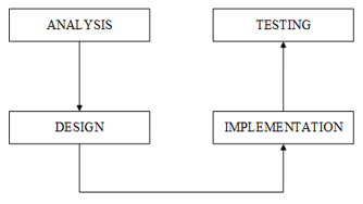
As can be seen in the Figure 1, the conventional procedure for this study was used [24].
Figure 1. Research methods
2.1 Analysis
Analysis is the skill of breaking complex issues or knowledge down into simpler, more understandable components. Parallel computing divides and executes big tasks simultaneously. Each little portion is broken into instructions, which are executed simultaneously on various processors. The implementation of parallel architecture is evaluated based on its performance in terms of speedup and efficiency and then compared to sequential computation [25, 26]. The formulae for speedup and efficiency are as follows:
$S=\frac{T s}{T p}$ (1)
$E=\frac{S}{p}$ (2)
The Gregory-Leibniz method converges very slowly; it takes approximately 5000 terms to compute π to three significant digits. In order to obtain more precise digits of π, it is necessary to perform a large number of term calculations in parallel computing [12].
2.2 Design
At this point, it will be detailed how the overall system design, the network topology employed for this study, and the specifics of each component. The network topology will be using regular star topology on a local area network with a switch mode mikrotik router Rb951series. High Level Design will be made as the premise for selecting the architecture to be implemented based on a variety of factors, including the use of each Raspberry Pis, the relationship between each Raspberry Pis, with the specifics of the employed technology [27] such as MPICH and MPI4Py [19]. The Low Level Design will be used to specify the MIMD parallel computing architecture that will be implemented in greater depth [28].
2.3 Implementation
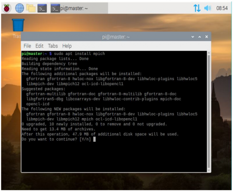
All procedures that have been developed will be used in this application phase, including software and hardware implementation [29]. The operating system used for the Raspberry Pis will be Raspbios Buster armhf. The Raspberry Pis with the mikrotik will be connected with an RJ45 cable. The configuration of mpich is required for the Raspberry Pis to recognize one another, and mpi4py will be installed so that Python programs can take advantage of MPI [30]. The command sudo apt install mpich must be entered in a terminal in order to install MPICH. The Gregory-Leibniz method uses arctan x series, the value of π could be calculated using the inverse tangent function, specifically arctan (1). The serial program would be calculate a certain ammount of terms of the arctan (1) series sequentially on one core of a processor. Meanwhile the parallel program will divide each of terms calculation to each core provided in the parallel computing architecture.
2.4 Testing
Table 1 describes the test scenarios that will be carried out in this study. The Gregory-Leibniz method of calculating Pi involves determining the infinite series of arctan x. Terms refers to the repetition of calculations based on the number of series. The greater the number of series, the more precise the Pi value achieved. The program will be performed on serial and parallel computers with the terms specified in Table 1. The program's execution time will be documented, and the findings will be used in the speedup and efficiency analysis parameters.
Table 1. Testing scenario
|
No. |
Scenarios |
Terms |
Parameters |
|
1 |
Serial (1 core) |
100,000; 500,000; 1,000,000; 5,000,000; 10,000,000; 20,000,000; 30,000,000; 40,000,000; 50,000,000 |
Speedup (S), Efficiency (E) |
|
2 |
Parallel with 1 Raspberry Pi (4 Core) |
||
|
3 |
Parallel with 2 Raspberry Pi (8 Core) |
||
|
4 |
Parallel with 3 Raspberry Pi (12 Core) |
In order to get findings that give a performance improvement by approximating the value of π in parallel, tests were conducted in this study utilizing some parameters. In studies [25, 26], the performance analysis of parallel computing uses two parameters namely speedup and efficiency. Speedup represents a metric for determining how much faster a parallel algorithm is compared to its sequential counterpart [3]. Speedup is defined as the ratio between the time required when employing a single processor core and the time measured when employing a specified number of processor cores. Efficiency is defined as the ratio of speedup to the number of cores utilized. Efficiency assesses the effectiveness with which a number of computers or CPUs are used in parallel computing [26]. The test conducted would include few scenarios, which are: executing and counting the time for each serial and parallel program with a calculated number of data or terms. The above table describes the test scenarios in greater detail.
This step refers to the outcome of each step that came before it and was performed successfully. The test results will include details on the execution of sequential and parallel programs, the time required for each program to complete, and performance improvement metrics like speedup and efficiency. These are the outcomes of the research’s conclusions.
3.1 Analysis
Insofar as necessary, the study will touch on current events. Tables 2 and 3 show that the needs analysis stage calls for supporting tools in order to do research on the subjects that will be covered.
Table 2. Hardware
|
No. |
Hardware |
Function |
|
1 |
Raspberry Pi 3B |
As a node in the MIMD parallel computing cluster system |
|
2 |
Raspberry Pi 3B+ |
As a node in the MIMD parallel computing cluster system |
|
3 |
Mikrotik Routerboard RB951series |
As a medium connecting one local network for each node and laptop |
Table 3. Software
|
No. |
Software |
Function |
|
1 |
Raspbios Buster Armhf |
The operating system used in carrying out the research. |
|
2 |
Balena Etcher |
Applications used to install the operating system |
|
3 |
PuTTY |
Application to remote access Raspberry Pi via SSH |
|
4 |
MPICH |
MPI Implementation |
3.2 Design
The design phase entails setting up a study setting that will support the goals and duties of the analysis phase while facilitating data collecting. In the design draft, the network topology and the MIMD parallel computing system are both described in general terms. An overview of the physical topology, high-level design, and low-level design are intended to be given at this design stage. The list appears below:
3.2.1 Network topology design
The routers, laptop clients, servers, and access points used in this study are depicted below.
The admin laptop has a dynamic IP address, whereas the Raspberry Pi that is linked has a static one. The access point router and the attached device communicate using a class C IP address.
Figure 2. Network topology design
Based on Figure 2, it is shown that the physical topology describes the design of the computer network structure within the scope of this research. Mikrotik RB951 series used with switch mode and access point as admin laptop access to the Raspberry Pi. Raspberry Pi node master is connected to the Mikrotik on port eth2. Raspberry Pi node slave1 is connected to the Mikrotik on port eth3. Raspberry Pi node slave2 is connected to the Mikrotik on port eth4. While connecting with the admin laptop, the Mikrotik is used in access point mode.
3.2.2 High level design
The system’s overall design is covered in this phase of the research process.
Figure 3. High level design
In Figure 3, the Multiple Instruction form carried out on the Raspberry Pi Node Master will have three instructions for each data processed, namely sending data, receiving data, and processing data again. Meanwhile, the Raspberri Pi Node Slave1 and Slave2 will receive data from the Node Master, process it, and send it back to the Node Master.
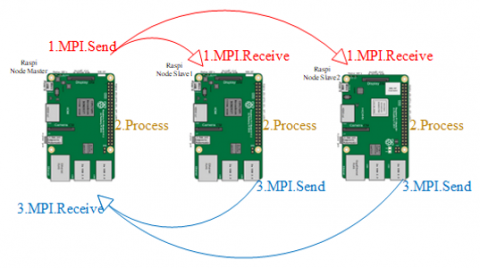
3.2.3 Low level design
This stage covers a thorough explanation of the system design, including how to use MIMD parallel computing to parallelize an π value calculation application.
Figure 4. Low level design
Figure 4 describes the design of the MIMD parallel computing structure applied to the Raspberry Pi. On the Raspberry Pi Node Master, the first instruction stage is to send the slice value to be processed on the Raspberry Pi Nodes Slave 1 and Slave 2. On Raspberry Pi Nodes Slave1 and Slave 2, the first instruction performed on the data is to receive data from the Node Master. After the data is received, the second instruction is to process the data according to the Gregory-Leibniz calculation method, and the last instruction is to send the processed data to the Raspberry Pi Node Master. The second instruction on the Raspberry Pi Node Master is to receive data that has been processed from the Raspberry Pi Node Slave 1 and Slave 2, then the third instruction is that the data received will be processed again so that the Pi value is obtained, and the last instruction is to display the Pi value obtained on the terminal.
3.3 Implementation
The analytical and design stages that were completed earlier continue with the implementation step. Researchers have broken this stage down into various sections.
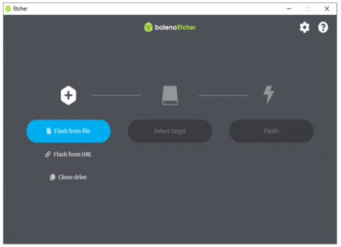
3.3.1 Operating system installation
BalenaEtcher program is used to install the operating system, which in this case is Raspberry Pi OS, into the SD Card.
Figure 5. Operating system installation
Figure 5 shows the process of BalenaEtcher installing the operating system on the SD card. To install the operating system onto the SD card, download the operating system file from the official Raspberry Pi page, then select the target SD card that will be used as the operating system storage medium, and finally click the Flash button and wait until the Flash process is complete.
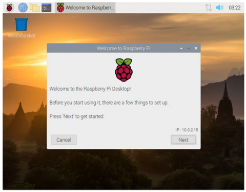
Figure 6. Setting display
Figure 6 shows when the Raspberry Pi first boots with the operating system successfully installed on the SD card. The Raspberry Pi must then be turned on until the first setup display appears, at which point users can change the factory-set password and enter information for the current location, language, and time zone.
3.3.2 MPICH installation
In order to enable message carrying interfaces in MIMD parallel computing, Message passing Interface (MPICH) was built as part of this research [18].
Figure 7. MPICH installation
Figure 7 shows the steps of MPICH installation. Installing MPICH is done by typing sudo apt install mpich on the terminal, then confirming by typing Y, then pressing the enter.
3.3.3 MPI4Py installation
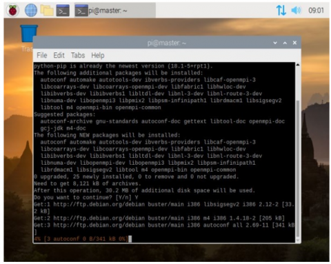
Researchers employ the Python programming language, which necessitates the use of a library initially. MPI4Py serves as the Python programming language’s Message Passing Interface binding. Any Python application can leverage many processors with the aid of MPI bindings [19]. Install the Python MPI library first by running sudo apt install python-pip python-dev libopenmpi-dev in the terminal and pressing enter. Once you’re done, execute sudo pip install mpi4py and hit enter.
Figure 8. MPI library installation
Figure 8 shows the steps of installing the Python MPI library by running sudo apt install python-pip python-dev libopenmpi-dev in the terminal and pressing enter.
Figure 9. MPI4Py installation
Figure 9 shows the steps of installing the MPI4Py by running sudo apt install mpi4py in the terminal and pressing enter
3.3.4 Sequential program implementation
The Gregory-Leibniz formula is adjusted in this study to account for the estimated value of Pi. James Gregory and Gottfried Wilhelm Leibniz, two prominent mathematicians from the 16th century, are known as Gregory-Leibniz. They developed the method for computing the value of π using an infinite series [10]. The arctan formula, developed by Gregory-Leibniz, is as follows:
$\arctan x=x-\frac{x^3}{3}+\frac{x^5}{5}-\frac{x^7}{7}+\cdots$ (3)
By using x=1 in the formula above, the Gregory-Leibniz π value formula is obtained as follows:
$\frac{\pi}{4}=1-\frac{1}{3}+\frac{1}{5}-\frac{1}{7}+\cdots$ (4)
Thus, an approximate value of π is obtained:
$\pi=4\left(1-\frac{1}{3}+\frac{1}{5}-\frac{1}{7}+\cdots\right)$ (5)
To approximate the value of π with a sequential program, the calculation is carried out by one processing unit sequentially based on each term of repetition of the calculation performed [24]. Table 4 shows the several Iteration of terms were carried out in this study.
Table 4. Sequential program test scenarios
|
No. |
Number of Processors |
Iteration/Terms |
|
1 |
1 |
100,000 |
|
2 |
1 |
500,000 |
|
3 |
1 |
1,000,000 |
|
4 |
1 |
5,000,000 |
|
5 |
1 |
10,000,000 |
|
6 |
1 |
20,000,000 |
|
7 |
1 |
30,000,000 |
|
8 |
1 |
40,000,000 |
|
9 |
1 |
50,000,000 |
3.3.5 Parallel program implementation
This study utilizes MIMD parallel computing to do a parallel calculation of the estimated value of π using the Gregory-Leibniz formula. The phases of parallelization are as follows:
Figure 10. Parallelization phases
Figure 10 shows the phases of parallel π estimation. Parallelization is done by dividing the calculation task of each iteration among the slave nodes.
Table 5 shows the numerous scenarios were carried out according to the iteration/terms [24] to estimate the value of π with a parallel program
Table 5. Parallel program test scenarios
|
No. |
Parallel Scenarios |
Terms |
|
1 |
1 Raspberry Pi (4 Core) |
100,000; 500,000; 1,000,000; 5,000,000; 10,000,000; 20,000,000; 30,00,000; 40,000,000; 50,000,000 |
|
2 |
2 Raspberry Pi (8 Core) |
|
|
3 |
3 Raspberry Pi (12 Core) |
3.4 Testing
The output of the program used to estimate π value in sequential and parallel runs will now be discussed.
3.4.1 Sequential approximation and time recording
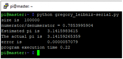
Utilizing the python gregory_leibniz-serial.py command, a sequential program may be run. The outcomes of running the program sequentially are showed in Figure 11.
Figure 11. Sequential program
The program is run nine times in accordance with the preset Terms, and the results are as follows:
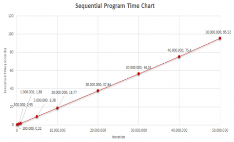
Table 6 shows the recorded program execution time for each scenario. It can be seen that as the number of terms increases, the more time it takes to execute the program.
Table 6. Sequential program test results
|
No. |
Terms |
Time (Ts) |
|
1 |
100,000 |
0,22 |
|
2 |
500,000 |
0,95 |
|
3 |
1,000,000 |
1,88 |
|
4 |
5,000,000 |
9,38 |
|
5 |
10,000,000 |
18,77 |
|
6 |
20,000,000 |
37,64 |
|
7 |
30,000,000 |
56,31 |
|
8 |
40,000,000 |
75,40 |
|
9 |
50,000,000 |
95,52 |
To make the comparison of program execution times simpler to grasp, Figure 12 shows a chart created using the previous table.
3.4.2 Parallel approximation and time recording
The mpi4py-n xx-machinefile machinefile gregory_leibniz-parallell.py command enables the execution of a parallel program. The outcomes of the parallel program execution are showed in Figure 13.
Figure 12. Sequential program time chart
Figure 13. Parallel program
The program is run nine times in accordance with the preset terms, and the results are as follows:
Table 7. Parallel program test results
|
No. |
Parallel Scenarios |
Terms |
Time (Tp) |
|
1 |
1 |
100,000 |
0,11 |
|
2 |
500,000 |
0,55 |
|
|
3 |
1,000,000 |
1,10 |
|
|
4 |
5,000,000 |
5,49 |
|
|
5 |
10,000,000 |
10,96 |
|
|
6 |
20,000,000 |
21,90 |
|
|
7 |
30,000,000 |
33,37 |
|
|
8 |
40,000,000 |
48,24 |
|
|
9 |
50,000,000 |
64,52 |
|
|
10 |
2 |
100,000 |
0,12 |
|
11 |
500,000 |
0,28 |
|
|
12 |
1,000,000 |
0,52 |
|
|
13 |
5,000,000 |
2,44 |
|
|
14 |
10,000,000 |
4,84 |
|
|
15 |
20,000,000 |
9,69 |
|
|
16 |
30,000,000 |
14,86 |
|
|
17 |
40,000,000 |
22,84 |
|
|
18 |
50,000,000 |
40,54 |
|
|
19 |
3 |
100,000 |
0,14 |
|
20 |
500,000 |
0,26 |
|
|
21 |
1,000,000 |
0,36 |
|
|
22 |
5,000,000 |
1,49 |
|
|
23 |
10,000,000 |
3,64 |
|
|
24 |
20,000,000 |
6,28 |
|
|
25 |
30,000,000 |
9,60 |
|
|
26 |
40,000,000 |
12,84 |
|
|
27 |
50,000,000 |
16,08 |
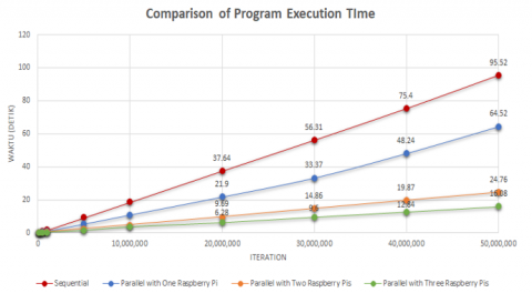
Table 7 shows the documented program execution time for each parallel program execution scenario. It can be seen that as the number of Rapsberry Pi used increases, the less time it takes to execute the program.
To help with comprehension of the comparison of program execution times, Figure 14 shows chart may be created using the created table:
Figure 14. Comparison of program execution time
3.4.3 Speedup and efficiency testing
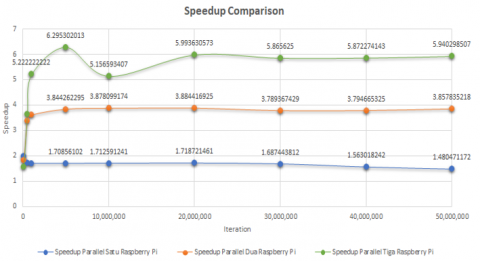
In order to compare the performance gain achieved, here is the speedup graph:
Figure 15. Speedup comparison chart
Figure 15 shows how speedup compares. On one Raspberry Pi running a parallel program. At 100,000 terms, the best speedup reached is 2. The best speedup in a parallel program running on two Raspberry Pis is 3.884416925 at 20,000,000 terms. The best speedup in a parallel program running on three Raspberry Pis is 6.295302013 at 5,000,000 terms. This means that when five million terms are calculated using three Raspberry Pis, the best speedup is obtained. The more Raspberry Pis and the more processing core is used the better speedup will be obtained.
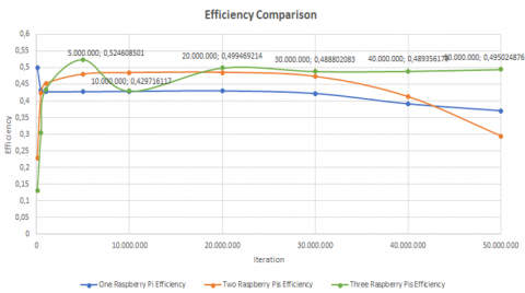
Figure 16. Efficiency comparison chart
Based on Figure 16 The efficiency corresponse to the speedup can be seen as follows: The best efficiency at the level of efficiency attained in the parallel program with one Raspberry Pi is 0.5 at 100,000 iterations. At the 20,000,000th iteration, the parallel program running on two Raspberry Pis achieved an efficiency level of 0.485552116. The best efficiency gained is 0.524608501 at the level of efficiency attained in the parallel program using three Raspberry Pis, and at iteration 5,000,000. The Raspberry Pi requires less electricity consumption than regular-sized desktop computers. This means sustainable energy sources, such as solar power [31] or wind power [32], could also be employed to provide electricity.
The findings of this research enable the drawing of several key conclusions: 1) The approximation of π values can indeed be parallelized, a process successfully demonstrated within this study. 2) The feasibility of employing Multiple Instruction Multiple Data (MIMD) parallel processing with a Raspberry Pi has been convincingly established. 3) A clear performance gain was observed when employing three Raspberry Pis, with the parameters of performance improvement exhibiting an increase corresponding to the number of Raspberry Pis utilized. A notable speedup of 6.2953020 was achieved, reducing the processing time from 9.38 seconds to 1.49 seconds at 5 million terms when three Raspberry Pis were in use. This discovery paves the way for further explorations of the Raspberry Pi in the development of cost-effective parallel computing architectures.
|
E |
Efficiency (dimensionless) |
|
p |
Number of parallel computing devices being used (dimensionless) |
|
S |
Speedup (dimensionless) |
|
Tp |
Parallel program execution time (second) |
|
Ts |
Sequential program execution time (second) |
|
π |
Mathematical constant that is the ratio of a circle's circumference to its diameter |
[1] Widayat, I.W., Irmawati, I., Syahrir, S.A.Q. (2017). Analisis sistem komputasi paralel pada infrastruktur grid computing. Jurnal Teknologi Elekterika, 14(1): 26. https://doi.org/10.31963/elekterika.v14i1.1213
[2] Rajpoot, V., Patel, A., Manepalli, P.K., Saxena, A. (2021). Deep learning and edge computing solution for high-performance computing. Deep Learning and Edge Computing Solutions for High Performance Computing, 1-18. https://doi.org/10.1007/978-3-030-60265-9_1
[3] Agapito, G., Guzzi, P.H., Cannataro, M. (2021). Parallel and distributed association rule mining in life science: A novel parallel algorithm to mine genomics data. Information Sciences, 575: 747-761. https://doi.org/10.1016/j.ins.2018.07.055
[4] Adamov, A.Z. (2020). Computation model of data intensive computing with mapreduce. In 2020 IEEE 14th International Conference on Application of Information and Communication Technologies (AICT), 1-5. https://doi.org/10.1109/AICT50176.2020.9368841
[5] Schmidt, B., González-Domínguez, J., Hundt, C., Schlarb, M. (2018). Modern architectures. Parallel Programming, 47-75. https://doi.org/10.1016/B978-0-12-849890-3.00003-4
[6] Marinescu, D.C. (2018). Parallel and distributed systems. Cloud Computing (Second edition), 113-150. https://doi.org/10.1016/B978-0-12-812810-7.00005-4
[7] Pandey, R., Badal, N. (2019). Understanding the role of parallel programming in multi-core processor based systems. In Proceedings of 2nd International Conference on Advanced Computing and Software Engineering (ICACSE).
[8] Song, C.X. (2021). Analysis on heterogeneous computing. Journal of Physics: Conference Series, 2031: 012049. https://doi.org/10.1088/1742-6596/2031/1/012049
[9] Doucet, K., Zhang, J. (2019). The creation of a low-cost raspberry pi cluster for teaching. In Proceedings of the Western Canadian Conference on Computing Education, 7: 1-5. https://doi.org/10.1145/3314994.3325088
[10] Swain, M. (2021). Two famous series for pi. At Right Angles, 10: 81-83.
[11] Damini, D.B., Dhar, A. (2020). How Archimedes showed that π is approximately equal to 22/7. arXiv Preprint arXiv: 2008.07995. https://doi.org/10.48550/arXiv.2008.07995
[12] Berggren, L., Borwein, J.M., Borwein, P.B. (1997). Pi: A source book. New York: Springer. https://doi.org/10.1007/978-1-4757-4217-6
[13] Alzer, H. (2019). A series representation for π. Elemente der Mathematik, 74(4): 176-178. https://doi.org/10.4171/em/395
[14] Dey, S. (2023). Some naive and computationally polished techniques to approximate π. Methodology, 1(2): 4. https://doi.org/10.13140/RG.2.2.10583.96167
[15] Nurmawati, E., Pangaribuan, R.H., Santoso, I. (2021). Comparison of serial and parallel computation on predicting missing data with EM algorithm. Jurnal Matematika, Statistika dan Komputasi, 18(1): 22-30. https://doi.org/10.20956/j.v18i1.14003
[16] Kanagachidambaresan, G.R. (2020). Role of edge analytics in sustainable smart city development: challenges and solutions. Scrivener Publishing LLC, 273-288. https://doi.org/10.1002/9781119681328
[17] DeFreez, D., Bhowmick, A., Laguna, I., Rubio-González, C. (2020). Detecting and reproducing error-code propagation bugs in MPI implementations. In Proceedings of the 25th ACM SIGPLAN Symposium on Principles and Practice of Parallel Programming, 187-201. https://doi.org/10.1145/3332466.3374515
[18] McDaniel, B., Lemley, E. (2022). Extended precision multiplication using a message passing interface (MPI). Journal of Computing Sciences in Colleges, 37(7): 62-69.
[19] Dalcin, L., Fang, Y.L.L. (2021). Mpi4py: Status update after 12 years of development. Computing in Science & Engineering, 23(4): 47-54. https://doi.org/10.1109/MCSE.2021.3083216
[20] Friadi, R., Junaidhi, J. (2019). Raspberry pi-based greenhouse light intensity, temperature, and humidity control system. Journal of Technopreneruship and Information Systems, 30-37. https://doi.org/10.36085/jtis.v2i1.217
[21] Putra, R.A., Sujana, A.P. (2019). Implementation of the cluster server on the raspberry pi using load balancing. Komputika: Jurnal Sistem Komputer, 8(1): 37-44. https://doi.org/10.34010/komputika.v8i1.1623
[22] Alex David, S., Ravikumar, S., Rizwana Parveen, A. (2018). Raspberry Pi in computer science and engineering education. In Intelligent Embedded Systems: Select Proceedings of ICNETS2, Springer Singapore, 11-16. https://doi.org/10.1007/978-981-10-8575-8_2
[23] Penyala, H., Ibrahim, S., El Mesalami, A. (2020). The raspberry pi education mine: for teaching engineering and computer science students concepts like, computer clusters, parallel computing, and distributed computing. In 2020 IEEE International Conference on Electro Information Technology (EIT), 624-628. https://doi.org/10.1109/EIT48999.2020.9208242
[24] Rohman, E.F., Ritzkal, R., Afrianto, Y. (2020). Fail path analysis on openflow network using floyd-warshall algorithm. Jurnal Mantik, 4(3): 1546-1550. https://doi.org/10.35335/mantik.Vol4.2020.959.pp1546-1550
[25] Lumbanraja, F.R., Aristoteles, A., Muttaqina, N.R. (2020). Analisa komputasi paralel mengurutkan data dengan metode radix dan selection. Jurnal Komputasi, 8(2): 77-93. https://doi.org/10.23960%2Fkomputasi.v8i2.2662
[26] Wibawa, I.P.A.P., Giriantari, I.D., Sudarma, M. (2018). Parallel computing using the message passing model on sim rs (hospital management information system). Makalah Ilmiah Teknologi Elektro, 17(3): 439-444. https://doi.org/10.24843/MITE.2018.v17i03.P20
[27] Kurniawan, D., Rustiati, E.L., Irawati, A.R., Muchlas, Z.Z.I. (2022). Pemantauan mentok rimba (asarcornis scutulata) berbasis sistem informasi geografis di taman nasional way kambas. Jurnal Pepadun, 3(1): 54-63. https://doi.org/10.23960/pepadun.v3i1.104
[28] Rahman, I.A., Ikbal, I. (2019). Perancangan litespeed cache menggunakan metode ppdioo di pt. ABC. Jurnal Ilmiah Komputer dan Informatika (KOMPUTA), 8(2): 62-69. https://doi.org/10.34010/KOMPUTA.V8I2.3051
[29] Pajankar, A. (2021). Introduction to raspberry pi. Practical Linux with Raspberry Pi OS: Quick Start, 1-34. https://doi.org/10.1007/978-1-4842-6510-9_1
[30] Wazir, S., Ikram, A.A., Imran, H.A., Ullah, H., Ikram, A.J., Ehsan, M. (2019) Performance comparison of mpich and mpi4py on raspberry pi-3b beowulf cluster. arXiv Preprint arXiv: 1911.03709. https://doi.org/10.48550/arXiv.1911.03709
[31] Abutaha, M., Amar, I., AlQahtani, S. (2022). Parallel and practical approach of efficient image chaotic encryption based on message passing interface (MPI). Entropy, 24(4): 566. https://doi.org/10.3390/e24040566
[32] Brungs, L., Kötter-Lange, K., Kottmeier, J., Poersch, R., Schweizer-Ries, P. (2021). How to foster fruitful collaborations – the impact of sustainability science. International Journal of Energy Production and Management, 6(4): 347-358. https://doi.org/10.2495/EQ-V6-N4-347-358