Osama M. Atyia*![]() | Fadhel S. Fadhel
| Fadhel S. Fadhel![]() | Mizal H. Alobaidi
| Mizal H. Alobaidi![]()
© 2023 IIETA. This article is published by IIETA and is licensed under the CC BY 4.0 license (http://creativecommons.org/licenses/by/4.0/).
OPEN ACCESS
This study unveils a novel approach, integrating the variational iteration method and numerical integration, to address the n-th order fuzzy random ordinary differential equations' linear fuzzy initial value problems. The robustness of the variational iteration method, a proven and reliable technique, ensures the effectiveness of the proposed approach. The sequence of approximations generated by this method is scrutinized to confirm its convergence towards the exact solution, demonstrating the method's precision. Two distinct examples, each with a different number of Brownian motion generations, are simulated to elucidate the practical application of the proposed approach. The outcomes affirm the method's reliability and efficiency in tackling such complex mathematical problems.
random differential equations, fuzzy differential equations, variational iteration method, Weiner process, fuzzy number
The concept of fuzzy sets and their fundamental principles were first proposed by Zadeh in 1965 [1]. Subsequently, in 1978, the inception of fuzzy ordinary differential equations (FODEs) was marked by Friedman et al. [2], who found their utility in diagnosing cosmic phenomena. Three types of FODEs were identified: one where fuzziness is apparent in the coefficients of the ordinary differential equation (ODE), another where the differential equation is crisp but the initial conditions are fuzzy, and the third where both the differential equation and the related initial conditions are fuzzy.
In recent years, the field of FODEs has witnessed significant advancements. Abbasbandy and Viranloo [3] in 2002 proposed a solution to fuzzy initial value problems (FIVP) using Taylor's method. Furthermore, Jafari et al. [4] in 2012 employed the variational iteration method (VIM) to resolve the n-th order linear and nonlinear systems of FODEs with fuzzy initial conditions. Allahvivallcoo et al. [5] in 2014 and Sadigh Behzadi et al. [6] in 2018 also used the VIM to solve nonlinear FODEs and the 2nd-order Abel-Volterra fuzzy integro-differential equation, respectively. In 2021, Fadhel and Sagban enhanced the VIM to yield more precise results and expedite the convergence of the approximate numerical solution towards the exact solution [7].
ODEs containing a stochastic process in their vector field are termed as random ordinary differential equations (RODEs). These equations are akin to stochastic ordinary differential equations (SODEs) based on Itô process, and find extensive applications in real-world scenarios. As noted by Han and Kloden [8], RODEs, which are sometimes considered special cases of stochastic models, remain of particular interest to the uncertainty qualification community.
The numerical solutions to RODEs based on the Euler difference scheme were first proposed by Cortés et al. [9] in 2007. Later in 2011, the same group of authors introduced a novel method for this equation [10]. In 2011 and 2016, Khudair et al. [11-13] used the VIM in conjunction with the Adomian decomposition method and homotopy analysis respectively to solve certain types of second-order RODEs. In 2017, Tchier et al. [14] investigated the mean and variance of the approximate solutions of the second-order RODEs with boundary conditions. Abdulsahib et al. [15] in 2019 amalgamated the VIM and numerical integration methods to evaluate the integral of the correction functional appearing in the VIM, thereby solving RODEs.
Fuzzy random ordinary differential equations (FRODEs) provide effective models for the dynamical systems of real-life phenomena, accounting for two kinds of uncertainties in the governing model: randomness and fuzziness [16-20]. The concept of fuzzy random variables, which can assume fuzzy numbers instead of crisp values, was first introduced and exemplified by Kwakernaak in 1978 [21]. Puri and Ralescu [22] in 1985 depicted the relationship between the outcome of a random experiment and imprecise data by defining a fuzzy random variable. Feng [23] in 2000 applied the concept of mean-square calculus to study the system of FSODEs. In 2007, Fei [24] examined the existence and uniqueness of the solution of FRODEs for Cauchy problem in a random fuzzy setting, and similar studies were conducted under the condition of Lipschitzean right-hand side by Malinowski in 2009 [25] and under generalized Lipschitz condition in 2012 [26]. According to Boswel and Taylor's 1987 study, the mean or sum of a group of independent fuzzy random variables converges to a fuzzy Gaussian random variable, thereby indicating a fuzzy counterpart to the central limit theorem of classical probability theory [27].
The VIM seems to be promising in solving FRODEs in comparison with other numerical methods, because of its efficiency and its simplicity in solving such type of equations.
In this paper, the main objective is to study FRODEs and then to find its approximate solution using the VIM, which is carried out and simulated for different number of generations of Brownian motion that are taken to be 100, 500 and 1000. The general form of the FRODEs that will be considered has the form:
$\begin{gathered}\tilde{x}^{(n)}(t ; \omega)=f\left(t, \tilde{x}(t ; \omega), \tilde{x}^{\prime}(t ; \omega), \ldots, \tilde{x}^{(n-1)}(t ; \omega)\right), t \in {\left[t_0, T\right], T \in \mathbb{R}}\end{gathered}$ (1)
with fuzzy initial conditions:
$\tilde{x}(t ; \omega)=x_0, \tilde{x}^{\prime}(\mathrm{t} ; \omega)=x_0^{\prime}, \ldots, \tilde{x}^{(n-1)}(\mathrm{t} ; \omega)=x_0^{n-1}$ (2)
where, w is the Weiner process and x(t;w) is a random fuzzy process.
In this section, the basic concepts related to this work will be presented, which are including essentially two topics, namely random process and then fuzzy logic.
2.1 Random variables concept
A random variable is a real-valued function X(ω), $\omega \in \Omega$, that is measurable in terms of the probability measure P, where Ω is the sample space [28, 29]. The family of random variables xt(ω) (or just xt or x(ω) or x(t, ω)) for two variables is called stochastic process. Assuming $\mathrm{t} \in\left[t_0, \mathrm{~T}\right] \subset[0, \infty), \omega \in \Omega$ has a common probability [30], then a stochastic Process Wt, for every $\mathrm{t} \in[0, \infty)$, is a Brownian motion or Wiener process if [31]:
1. $P\left(\left\{\omega \in \Omega \mid w_0(\omega)=0\right\}\right)=1$.
2. For $0<t_0<t_1<\ldots<, t_3$ the increments $W_{t_1}-W_{t_0}, W_{t_2}-$ $W_{t_1}, \ldots, W_{t_n}-W_{t_{n-1}}$ are independent.
3. For an arbitrary t and h>0, then Wt+h-Wt has a normal distribution with mean 0 and variance h.
It is possible to study the convergence of the sequence of random variables denoted by $\left\{x_n(\omega)\right\}$, $\mathrm{n} \in \mathbb{N}$, using a variety of methods. One of these methods is known as converges with probability one. (Denoted by P-w.p.1 or w.p.1), which is also referred to as almost sure convergence (for short a.s.) if:
$P\left(\left\{\omega \in \Omega: \lim _{n \rightarrow \infty} x_n(\omega)=x(\omega)\right\}\right)=1$
Also, another type of convergence is the converges in probability to x(ω), which satisfies for all $\varepsilon>0$ [29]:
$\lim _{n \rightarrow \infty} P\left(\left\{\omega \in \Omega:\left|x_n(\omega)-x(\omega)\right| \geq \varepsilon\right\}\right)=0$
2.2 Fuzzy set theory
Fuzzy set theory is a generalization of the classical or crisp sets. Suppose that X is the universal set, which is nonempty and $\tilde{A}$ be a fuzzy subset of X, the function $\mu_{\tilde{A}}$ is used to denote the membership function or the grades of an element x which belongs to $\tilde{A}$, which is a real valued function from X onto the unit interval [0,1]. The fuzzy set $\tilde{A}$ can be represented as a set of ordered pairs in the form [32]:
$\tilde{A}=\left\{\left(x, \mu_{\tilde{A}}(x)\right): x \in X, \mu_{\tilde{A}}(x) \in[0,1]\right\}$.
Fuzzy numbers (FN) are special cases of a fuzzy sets, which is defined over the field of real numbers $\mathbb{R}$. In addition, among the main notations in fuzzy set theory, which are of importance in this work, are the a-cut or a-level of a fuzzy set $\tilde{A}$ is the set of all $\mathrm{x} \in \mathrm{X}$, such that $\mu_{\tilde{A}}(x) \geq \alpha$. Convex fuzzy set if:
$\mu_{\tilde{A}}(\lambda x+(1-\lambda) y) \geq \min \left\{\mu_{\tilde{A}}(x), \mu_{\tilde{A}}(y)\right\}$,
for all $\lambda \in[0,1]$, while normal fuzzy sets are those sets with maximum membership value equals 1, otherwise it may be normalized. Thus, a fuzzy number assumed to be convex normalized fuzzy subset $\tilde{A}$ of $\mathbb{R}$ with a piecewise continuous membership function [32].
Again, an arbitrary FN may be represented in parametric form using a-level sets as an ordered pair of functions $(\underline{u}(\alpha), \bar{u}(\alpha)), \quad 0 \leq \alpha \leq 1$; which satisfy the following requirements [33]:
(i) $\underline{u}(\alpha)$ is a bounded right continuous non-decreasing function over [0,1].
(ii) $\bar{u}(\alpha)$ is a bounded left continuous non-increasing function over [0,1].
(iii) $\underline{u}(\alpha) \leq \bar{u}(\alpha) ; 0 $\tilde{v}=(\underline{v}(\alpha), \bar{v}(\alpha))$\leq \alpha \leq 1:$
A crisp number a is simply represented by $\underline{u}(\alpha)=\bar{u}(\alpha)=\mathrm{a}$; $0 \leq \alpha \leq 1$ and for an arbitrary two fuzzy numbers $\tilde{u}=$ $(u(\alpha) ; \bar{u}(\alpha))$ and $\tilde{v}=(\underline{v}(\alpha), \bar{v}(\alpha))$, the following algebraic operations may be carried on:
(a) $\tilde{u}=\tilde{v}$ if and only if $\underline{u}(\alpha)=\underline{v}(\alpha)$; and $\bar{u}(\alpha)=\bar{v}(\alpha)$.
(b) $\tilde{u} \oplus \tilde{v}=(\underline{u \oplus v} ; \overline{u \oplus v})=(\underline{u}(\alpha)+(\underline{v}(\alpha) ; \bar{u}(\alpha)+\bar{v}(\alpha))$.
(c) $k \odot \tilde{u}=\left\{\begin{array}{l}(\underline{k \odot u}, \overline{k \odot u})=(k \underline{u}(\alpha), k \bar{u}(\alpha)), k \geq 0 \\ \left(\underline{k \odot u}, \overline{k \odot u}\right)=(k \bar{u}(\alpha), k \underline{u}(\alpha)), k<0\end{array}\right.$
Now, the general form of the n-th order FRODE with constant coefficients related to Eq. (1) is given [34, 35]:
$\begin{aligned} \tilde{x}^{(n)}(t, \omega)+c_{n-1} \, \tilde{x}^{(n-1)}(t, \omega) & +\cdots+c_1 \tilde{x}^{\prime}(t, \omega) +c_0 \tilde{x}(t, \omega)=\widetilde{R}(t, \omega), t \geq 0\end{aligned}$ (3)
with initial conditions:
$\tilde{x}(0, \omega)=\tilde{b}_0, \tilde{x}^{\prime}(0, \omega)=\tilde{b}_1, \ldots, \tilde{x}^{(n-1)}(0, \omega)=\tilde{b}_{n-1}$
where, all $0 \leq i \leq n-1$ have real constants called ci's and $\tilde{x}$ is the solution that will be described as a fuzzy function, $\tilde{b}_i$, for all $i$ $=0,1, \ldots, n-1$ are triangular fuzzy numbers and $\widetilde{R}$ is any given function plays the role of the nonhomgeneuous term.
Also, we can write Eq. (3) in the terms of lower and upper solutions, which is related to the a-levels of the fuzzy solution, and is given as:
$\begin{gathered}(\left.\underline{x}^{(n)}(t ; \omega, \alpha), \bar{x}^{(n)}(t ; \omega, \alpha)\right.)+ \\ c_{n-1}\left(\underline{x}^{(n-1)}(t ; \omega, \alpha), \bar{x}^{(n-1)}(t ; \omega, \alpha)\right) \\ +\cdots+c_1\left(\underline{x}^{\prime}(t ; \omega, \alpha), \overline{x^{\prime}}(t ; \omega, \alpha)\right) \\ +c_0(\underline{x}(t ; \omega, \alpha), \bar{x}(t ; \omega, \alpha)) \\ =(\underline{R}(t ; \omega, \alpha), \bar{R}(t ; \omega, \alpha))\end{gathered}$ (4)
Thus, three cases related to Eq. (3) are considered depending on the linear coefficients of the differential equation [34, 36, 37]:
Case (i): When all of the coefficients in Eq. (4), from $c_{n-1}, c_{n-2}, \ldots, c_1, c_0$, are positive. Next, the new equations are rewritten in terms of the lower and upper bounds as:
$\begin{gathered}\underline{x}^{(n)}(t ; \omega, \alpha)+c_{n-1} \underline{x}^{(n-1)}(t ; \omega, \alpha)+\cdots+ \\ c_1 \underline{x}^{\prime}(t ; \omega, \alpha)+c_0 \underline{x}(t ; \omega, \alpha)=\underline{R}(t ; \omega, \alpha), t \geq 0, \alpha \in {[0,1]}\end{gathered}$ (5)
with initial conditions:
$\underline{x}(0, \omega, \alpha)=\underline{b}_0, \underline{x}^{\prime}(0, \omega, \alpha)=\underline{b}_1, \ldots, \underline{x}^{(n-1)}(0, \omega, \alpha)=\underline{b}_{n-1}$
and:
$\begin{aligned} \bar{x}^{(n)}(t ; \omega, \alpha)+c_{n-1}\, \bar{x}^{(n-1)}(t ; \omega, \alpha)+\cdots +c_1 \overline{x^{\prime}}(t ; \omega, \alpha)+c_0 \bar{x}(t ; \omega, \alpha) =\bar{R}(t ; \omega, \alpha)\end{aligned}$ (6)
with initial conditions:
$\bar{x}(0 ; \omega, \alpha)=\bar{b}_0, \bar{x}^{\prime}(0 ; \omega, \alpha)=\bar{b}_1, \ldots, \bar{x}^{(n-1)}(0 ; \omega, \alpha)=\bar{b}_{n-1}$
Case (ii): When some of the coefficients in Eq. (4), say $c_{m-1}\, , \ldots, c_{m-n}$ are positive and $c_{m-n-1}\,\, , c_{m-n-2}\,\, , \ldots, c_1, c_0$ are negative, then one may obtain the lower- and upper-bound equations as:
If some of the coefficients in Eq. (4), such as $c_{m-1}\, , \ldots, c_{m-n}$, have positive values, but other coefficients in the equation, such as $c_{m-n-1}\,\, , c_{m-n-2}\,\, , \ldots, c_1, c_0$ have negative values and so the equations for the lower and upper bounds may be written as follows:
$\begin{gathered}\underline{x}^{(n)}(t ; \omega, \alpha)+c_{n-1} \underline{x}^{(n-1)}(t ; \omega, \alpha)+\cdots+ \\ c_{n-m} \underline{x}^{(n-m)}(t ; \omega, \alpha)+c_{n-m-1}\,\, \bar{x}^{(n-m-1)}\, (t ; \omega, \alpha)+ \\ \cdots+c_0 \bar{x}(t ; \omega, \alpha)=\underline{R}(t ; \omega, \alpha), t \geq 0, \alpha \in[0,1]\end{gathered}$ (7)
with initial conditions:
$\begin{gathered}\underline{x}^{(n-1)}\, (0 ; \omega, \alpha)=\underline{b}_{n-1}, \ldots, \underline{x}^{(n-m)}(0 ; \omega, \alpha)=\underline{b}_{n-m} \, , \\ \bar{x}^{(n-m-1)}\, (0 ; \omega, \alpha)=\bar{b}_{n-m-1}\, , \ldots, \bar{x}^{\prime}(0 ; \omega, \alpha)=\bar{b}_1, \bar{x}(0 ; \omega, \alpha) =\bar{b}_0\end{gathered}$
and the upper solution:
$\begin{gathered}\bar{x}^{(n)}(t ; \omega, \alpha)+c_{n-1} \bar{x}^{(n-1)}\, (t ; \omega, \alpha)+\cdots+ \\ c_{n-m} \bar{x}^{(n-m)}(t ; \omega, \alpha)+c_{n-m-1}\, \underline{x}^{(n-m-1)}\, (t ; \omega, \alpha)+ \\ \cdots+c_0 \underline{x}(t ; \omega, \alpha)=\bar{R}(t ; \omega, \alpha)\end{gathered}$ (8)
with initial conditions:
$\begin{gathered}\bar{x}^{(n-1)}(0 ; \omega, \alpha)=\bar{b}_{n-1}, \ldots, \bar{x}^{(n-m)}(0 ; \omega, \alpha)= \\ \bar{b}_{n-m} \underline{x}^{(n-m-1)}(0 ; \omega, \alpha)=\underline{b}_{n-m-1}, \ldots, \underline{x}^{\prime}(0 ; \omega, \alpha)= \\ \underline{b}_1, \underline{x}(0 ; \omega, \alpha)=\underline{b}_0\end{gathered}$
Case (iii): When all of the coefficients in the Eq. (4), $c_{n-1}, c_{n-2}, \ldots, c_1, c_0$, are negative. Then after, we will be able to obtain the lower- and upper-bound equations that are as follows:
$\begin{gathered}\underline{x}^{(n)}(t ; \omega, \alpha)+c_{n-1} \bar{x}^{(n-1)}(t ; \omega, \alpha)+\cdots+ \\ c_1 \bar{x}^{\prime(t ; \omega, \alpha)}+c_0 \bar{x}(t ; \omega, \alpha)=\underline{R}(t ; \omega, \alpha), t \geq 0, \alpha \in[0,1]\end{gathered}$ (9)
with initial conditions:
$\bar{x}(0, \omega, \alpha)=\bar{b}_0, \bar{x}^{\prime}(0, \omega, \alpha)=\bar{b}_1, \ldots, \bar{x}^{(n-1)}(0, \omega, \alpha)=\bar{b}_{m-1}$
and
$\begin{gathered}\bar{x}^{(n)}(t ; \omega, \alpha)+c_{n-1} \underline{x}^{(n-1)}(t ; \omega, \alpha)+\cdots+ \\ c_1 \underline{x}^{\prime}(t ; \omega, \alpha)+c_0 \underline{x}(t ; \omega, \alpha)=\bar{R}(t ; \omega, \alpha)\end{gathered}$ (10)
and the initial conditions:
$\underline{x}(0 ; \omega, \alpha)=\underline{b}_0, \underline{x}^{\prime}(0 ; \omega, \alpha)=\underline{b}_1, \ldots, \underline{x}^{(n-1)}(0 ; \omega, \alpha)=\underline{a}_{n-1}$
It is notable that there are no certain scenario applications for the above three cases, except that the application of these cases depends on the signs of the coefficients $c_{n-1}, c_{n-2}, \ldots, c_1, c_0$ in Eq. (3).
In order to solve the FRODEs given in general by Eq. (1) and in particular by Eq. (3) with fuzzy initial conditions given by Eq. (2) using the VIM, first we have to rewrite Eq. (1) in an operator form as:
$L\{\tilde{x}(t ; \omega)\}+N\{\tilde{x}(t ; \omega)\}=g(t ; \omega)$ (11)
where, L is a linear operator, N is a nonlinear operator [7], g is a known analytical function. The approximate solution by using the VIM will be in the form as in the following correction functional:
$\begin{gathered}\tilde{x}_{m+1}(t ; \omega)=\tilde{x}_m(t ; \omega)+\int_{t_0}^T \lambda(s, t)\left\{L\left\{\tilde{x}_m(s ; \omega)\right\}+\right. \left.N\left\{\tilde{x}_m(s ; \omega)\right\}-g(s ; \omega)\right\} d s\end{gathered}$ (12)
where, $\tilde{x}_m$ is the restricted variations, i.e., the first variation $\delta \tilde{x}_m=0$ and $\lambda$ is the general Lagrange multiplier which was identified optimally using variational theory and it is proved in literatures (see for example [38, 39]) to be in the form of the n-th order ordinary differential equation:
$\lambda(s, t)=(-1)^n \frac{(s-t)^{n-1}}{(n-1) !}$ (13)
where, $n \in \mathbb{N}$. therefore, the solution of iteration Eq. (12) will be after taken the general Lagrange multiplier (13) with fuzzy initial condition $\tilde{x}_0$ related to the nonlinear operator Eq. (11) will be in the form:
$\tilde{x}_{m+1}(t ; \omega)=\tilde{x}_m(t ; \omega)+\int_{t_0}^T(-1)^n \frac{(s-t)^{n-1}}{(n-1) !}$
$\left\{\mathrm{L}\left\{\tilde{x}_m(s ; \omega)\right\}+N\left\{\tilde{x}_m(s ; \omega)\right\}-g(s ; \omega)\right\} d s$ (14)
Again, the approximate solution of the general form of n-th order of RFODEs with constant coefficients using the VIM is given by:
$\begin{gathered}\tilde{x}_{m+1}(t ; \omega)=\tilde{x}_m(t ; \omega)+\int_{t_0}^T(-1)^n \frac{(s-t)^{n-1}}{(n-1) !} \\ \left\{\tilde{x}_m^{(n)}(s, \omega)+c_{n-1} \tilde{x}_m^{(n-1)}(s, \omega)+\cdots+c_1 \tilde{x}_m^{\prime}(s, \omega)+\right. \left.c_0 \tilde{x}_m(s, \omega)-\tilde{R}(s, \omega)\right\} d s\end{gathered}$ (15)
Also, the following three cases are considered for the sequence of the approximate solution using VIM:
Case (i): When each one of the coefficients $c_{n-1}, c_{n-2}, \ldots, c_1, c_0$ is positive. The correction functional for solving Eq. (3) using VIM for every iteration m=0, 1, 2, … is given as:
$\begin{aligned} & \underline{x}_{m+1}(t ; \omega, \alpha)=\underline{x}_m(t ; \omega, \alpha)+\frac{(-1)^n}{(n-1) !} \int_{t_0}^T(s-t)^{n-1}\left\{\underline{x}_m^{(n)}(s ; \omega, \alpha)+c_{n-1} \underline{x}_m^{(n-1)}(s ; \omega, \alpha)+\cdots+\right. \\ & \left.c_1 \underline{x}^{\prime}(s ; \omega, \alpha)+c_0 \underline{x}(s ; \omega, \alpha)-R(s ; \omega, \alpha)\right\} d s\end{aligned}$ (16)
$\begin{gathered}\bar{x}_{m+1}(t ; \omega, \alpha)=\bar{x}_m(t ; \omega, \alpha)+\frac{(-1)^n}{(n-1) !} \int_{t_0}^T(s-t)^{n-1}\left\{\bar{x}_m^{(n)}(s ; \omega, \alpha)+c_{n-1} \bar{x}_m^{(n-1)}(s ; \omega, \alpha)+\cdots+\right. \\ \left.c_1 \bar{x}^{\prime}(s ; \omega, \alpha)+c_0 \bar{x}(s ; \omega, \alpha)-\bar{R}(s ; \omega, \alpha)\right\} d s\end{gathered}$ (17)
Case (ii): When some of the coefficients $c_{n-1}\, , \ldots, c_{n-m}$ have a positive value while the other coefficients $c_{n-m-1}\,\, , c_{n-m-2}\,\, , \ldots, c_1, c_0 ; m, n \in \mathbb{N}$ have negative value. Then, the correction functional for solving Eq. (3) using VIM for all iteration m=0, 1, … is given as:
$\begin{gathered}\underline{x}_{m+1}(t ; \omega, \alpha)=\underline{x}_m(t ; \omega, \alpha)+\frac{(-1)^n}{(n-1) !} \int_{t_0}^T(s-t)^{n-1}\left\{\underline{x}_m^{(n)}(s ; \omega, \alpha)+c_{n-1} \underline{x}_m^{(n-1)}(s ; \omega, \alpha)+\cdots+\right. \\ c_{n-m} \underline{x}_m^{(n-m)}(s ; \omega, \alpha)+c_{n-m-1}\, \bar{x}_m^{(n-m-1)}(s ; \omega, \alpha)+ \\ \left.\cdots+c_0 \bar{x}_m(s ; \omega, \alpha)-\underline{R}(s ; \omega, \alpha)\right\} d s\end{gathered}$ (18)
$\begin{gathered}\bar{x}_{m+1}(t ; \omega, \alpha)=\bar{x}_m(t ; \omega, \alpha)+\frac{(-1)^n}{(n-1) !} \int_{t_0}^T(s-t)^{n-1}\left\{\bar{x}_m^{(n)}(s ; \omega, \alpha)+\right. \\ c_{n-1} \bar{x}_m^{(n-1)}(s ; \omega, \alpha)+\ldots+c_{n-m} \bar{x}_m^{(n-m)}(s ; \omega, \alpha)+ \\ c_{n-m-1}\, \underline{x}_m^{(n-m-1)}\, (s ; \omega, \alpha)+\cdots+c_0 \underline{x}_m(s ; \omega, \alpha)- \\ \bar{R}(s ; \omega, \alpha)\} d s\end{gathered}$ (19)
Case (iii): When all of the coefficients $c_{n-1}, c_{n-2}, \ldots, c_1, c_0$ are negative. Then, the correction functional for solving Eq. (3) using VIM for all iteration m=0, 1, … is given as:
$\begin{gathered}\underline{x}_{m+1}(t ; \omega, \alpha)=\underline{x}_m(t ; \omega, \alpha)+\frac{(-1)^n}{(n-1) !} \int_{t_0}^T(s-t)^{n-1}\left\{\underline{x}_m^{(n)}(s ; \omega, \alpha)+c_{n-1} \bar{x}_m^{(n-1)}(s ; \omega, \alpha)+\cdots+\right. \\ \left.c_1 \bar{x}_m^{\prime}(s ; \omega, \alpha)+c_0 \bar{x}_m(s ; \omega, \alpha)-\underline{R}(s ; \omega, \alpha)\right\} d s\end{gathered}$ (20)
In the previous section, we had presented an alternative approach of the VIM [40] for solving FRODEs, which can be used, in an effective and reliable way to handle the FRODEs in operator form given by Eq. (11). Thus, in this section, and according to the above three cases, we will consider only the convergence of the first case of the approximation using VIM (15) to the exact solution of the FRODEs (1), however the other two cases may be verified similarly.
When all the coefficients $c_0, c_1, \ldots, c_{n-1}$ are positive. Then the correction functional to be determined as an approximate solution to the problem under consideration using the VIM for all m=0, 1, … consists of the following lower and upper solutions:
$\begin{gathered}\underline{x}_{m+1}(t ; \omega, \alpha)=\underline{x}_m(t ; \omega, \alpha)+\frac{(-1)^n}{(n-1) !} \int_{t_0}^T(s- \\ t)^{n-1}\left\{\underline{x}_m^{(n)}(s ; \omega, \alpha)+c_{n-1} \underline{x}_m^{(n-1)}(s ; \omega, \alpha)+\cdots+\right. \\ \left.c_1 \underline{x}_m^{\prime}(s ; \omega, \alpha)+c_0 \underline{x}_m(s ; \omega, \alpha)-\underline{R}(s ; \omega, \alpha)\right\} d s \\ \bar{x}_{m+1}(t ; \omega, \alpha)=\bar{x}_m(t ; \omega, \alpha)+\frac{(-1)^n}{(n-1) !} \int_{t_0}^T(s- \\ t)^{n-1}\left\{\bar{x}_m^{(n)}(s ; \omega, \alpha)+c_{n-1} \bar{x}_m^{(n-1)}(s ; \omega, \alpha)+\cdots+\right. \\ \left.c_1 \bar{x}_m^{\prime}(s ; \omega, \alpha)+c_0 \bar{x}_m(s ; \omega, \alpha)-\bar{R}(s ; \omega, \alpha)\right\} d s\end{gathered}$
The above FRODEs is given subjected to the following initial conditions:
$\bar{x}^k(0 ; \omega, \alpha)=\bar{x}_0^k, k=0,1, \ldots, n-1$ (21)
$\underline{x}^k(0 ; \omega, \alpha)=\underline{x}_0^k, k=0,1, \ldots, n-1$ (22)
where, $\bar{x}_0^k$ and $\underline{x}_0^k$ are given real numbers for all k = 0, 1, …, n - 1
Simply, we will consider the convergence analysis for the upper case and the following operator is defined to be used in the proof, which depends on the Banach fixed point theorem:
$\begin{gathered}A(\bar{x}(t ; \omega, \alpha))=\frac{(-1)^n}{(n-1) !} \int_{t_0}^T(s-t)^{n-1}\left\{\bar{x}_m^{(n)}(s ; \omega, \alpha)+\right. \\ c_{n-1} \bar{x}_m^{(n-1)}(s ; \omega, \alpha)+\cdots+c_1 \bar{x}_m^{\prime}(s ; \omega, \alpha)+ \\ \left.c_0 \bar{x}_m(s ; \omega, \alpha)-\bar{R}(s ; \omega, \alpha)\right\} d s\end{gathered}$ (23)
Also, define the following new components $\bar{v}_k$ $(t ; \omega, \alpha)$, k = 0, 1, …; as follows:
$\begin{gathered}\bar{v}_0(t ; \omega, \alpha)=\bar{x}_0(t ; \omega, \alpha)=\bar{x}_0 \\ \bar{v}_1(t ; \omega, \alpha)=A\left[\bar{v}_0(t ; \omega, \alpha)\right] \\ \bar{v}_2(t ; \omega, \alpha)=A\left[\bar{v}_0(t ; \omega, \alpha)+\bar{v}_1(t ; \omega, \alpha)\right] \\ \vdots \\ \bar{v}_{k+1}(t ; \omega, \alpha)=\mathrm{A}\left[\bar{v}_0(t ; \omega, \alpha)+\bar{v}_1(t ; \omega, \alpha)+\ldots+\right. \left.\bar{v}_k(t ; \omega, \alpha)\right]\end{gathered}$ (24)
Hence, for the convergence of the VIM, one must have:
$\begin{gathered}\bar{x}(t ; \omega, \alpha)=\lim _{k \rightarrow \infty} \bar{x}_k(t ; \omega, \alpha) \\ =\sum_{k=0}^{\infty} \bar{v}_k(t ; \omega, \alpha)\end{gathered}$
Thus, the solution of problem (11) may be obtained using the following series:
$\bar{x}(t ; \omega, \alpha)=\sum_{k=0}^{\infty} \bar{v}_k(t ; \omega, \alpha)$ (25)
The zeroth (initial guess) approximation $\bar{v}_0(t ; \omega, \alpha)=\bar{x}_0(t ; \omega, \alpha)=\bar{x}_0$ can be freely chosen if it satisfies the initial requirements, as well as, the boundary conditions of the problem that is being considered. The success of the fast convergence of the approximate solution to the exact solution depends on the proper selection of the initial approximation $\bar{v}_0$ (t; w, $\alpha$). However, using the initial values $\bar{x}^k(0 ; \omega, \alpha)=\bar{x}_0^k, k=0,1, \ldots, n-1$ are preferably used for the selective zeroth approximation $\bar{v}_0(t ; \omega, \alpha)$ as will be seen later. In an alternative approach, and for simplicity, one can select the initial approximation $\bar{v}_0(t ; \omega, \alpha)$ as:
$\bar{v}_0(t ; \omega, \alpha)=\sum_{k=0}^{\infty} \frac{\bar{x}_0^k}{k!}(t ; \omega, \alpha)$ (26)
As a result, the shortened series up to the m-terms can approximate the exact solution as:
$\bar{x}(t ; \omega, \alpha)=\sum_{k=0}^{\infty} \bar{v}_k(t ; \omega, \alpha)$
For the convergence of the VIM when the alternative method described above is used to solve Eq. (11), in which the sufficient condition of the method and the error estimate are presented. The following theorem is a special case of the Banach fixed point theorem with random variables and fuzzy initial conditions.
Theorem (1): Consider the operator (23) given by:
$\begin{gathered}A(\bar{x}(t ; \omega, \alpha))=\frac{(-1)^n}{(n-1) !} \int_{t_0}^T(s-t)^{n-1}\left\{\bar{x}_m^{(n)}(s ; \omega, \alpha)+\right. \\ c_{n-1} \bar{x}_m^{(n-1)}(s ; \omega, \alpha)+\cdots+c_1 \bar{x}_m^{\prime}(s ; \omega, \alpha)+c_0 \bar{x}_m(s ; \omega, \alpha)- \bar{R}(s ; \omega, \alpha)\} d s\end{gathered}$
to be defined by transforming a Hilbert space H into itself. The series solution is then $\bar{x}(t ; \omega, \alpha)=\sum_{k=0}^{\infty} \bar{v}_k(t ; \omega, \alpha)$ converges if there exists $\gamma \in(0,1)$, such that:
$\begin{gathered}|| A\left[\bar{v}_0(t ; \omega, \alpha)+\bar{v}_1(t ; \omega, \alpha)+\ldots+\bar{v}_{k+1}(t ; \omega, \alpha)\right] \| \leq \\ \gamma\left\|A\left[\bar{v}_0(t ; \omega, \alpha)+\bar{v}_1(t ; \omega, \alpha)+\ldots+\bar{v}_k(t ; \omega, \alpha)\right]\right\|\end{gathered}$
that is:
$\left\|\bar{v}_{k+1}(t ; \omega, \alpha)\right\| \leq \gamma\left\|\bar{v}_k(t ; \omega, \alpha)\right\|, \forall k=0,1, \ldots$
Proof: Define the sequence $\left\{\bar{s}_m(t ; \omega, \alpha)\right\}_{m=0}^{\infty}$ as:
$\left.\begin{array}{rl}\bar{s}_0= & \bar{v}_0(t ; \omega, \alpha) \\ \bar{s}_1= & \bar{v}_0(t ; \omega, \alpha)+\bar{v}_1(t ; \omega, \alpha) \\ \bar{s}_2= & \bar{v}_0(t ; \omega, \alpha)+\bar{v}_1(t ; \omega, \alpha)+\bar{v}_2(t ; \omega, \alpha) \\ & \vdots \\ \bar{s}_m= & \bar{v}_0(t ; \omega, \alpha)+\bar{v}_1(t ; \omega, \alpha)+\cdots+ \bar{v}_m(t ; \omega, \alpha)\end{array}\right\}$ (27)
and hence to show that $\left\{\bar{s}_m(t ; \omega, \alpha)\right\}_{m=0}^{\infty}$ is a Cauchy sequence in the Hilbert space H. For this purpose, consider $m \in \mathbb{N}$, then:
$\begin{aligned}\left\|\bar{s}_{m+1}-\bar{s}_m\right\|= & \left\|\bar{v}_{m+1}(t ; \omega, \alpha)\right\| \\ & \leq \gamma\left\|\bar{v}_m(t ; \omega, \alpha)\right\| \\ & \leq \gamma^2\left\|\bar{v}_{m-1}(t ; \omega, \alpha)\right\| \\ & \vdots \\ \leq & \gamma^{m+1}\left\|\bar{v}_0(t ; \omega, \alpha)\right\|\end{aligned}$ (28)
Now, for every $m, j \in \mathbb{N}, m \geq j$, we have:
$\begin{aligned} & \left\|\bar{s}_m-\bar{s}_j\right\|=\|\left(\bar{s}_m-\bar{s}_{m-1}\right)+\left(\bar{s}_{m-1}-\bar{s}_{m-2}\right)+\ldots+ \quad\left(\bar{s}_{j+1}-\bar{s}_j\right) \| \\ & \leq\left\|\bar{s}_m-\bar{s}_{m-1}\right\|+\left\|\bar{s}_{m-1}-\bar{s}_{m-2}\right\|+\ldots+\left\|\bar{s}_{j+1}-\bar{s}_j\right\| \\ & \leq \gamma^m\left\|\bar{v}_0(t ; \omega, \alpha)\right\|+\gamma^{m-1}\left\|\bar{v}_0(t ; \omega, \alpha)\right\|+\ldots+ \\ & \gamma^{j+1}\left\|\bar{v}_0(t ; \omega, \alpha)\right\| \leq \frac{1-\gamma^{m-j}}{1-\gamma} \gamma^{j+1}\left\|\bar{v}_0(t ; \omega, \alpha)\right\|\end{aligned}$ (29)
and since 0<g<1, then:
$\lim _{j m \rightarrow \infty}\left\|\bar{s}_m(t ; \omega, \alpha)-\bar{s}_j(t ; \omega, \alpha)\right\|=0$ (30)
Therefore, $\left\{\bar{s}_m(t ; \omega, \alpha)\right\}_{m=0}^{\infty}$ is a Cauchy sequence in the Hilbert space $H$, which implies that the series solution $\bar{x}(t ; \omega, \alpha)=\sum_{k=0}^{\infty} \bar{v}_k(t ; \omega, \alpha)$ defined in Eq. (25) will be converge to the exact solution.
Theorem (2): The solution $\sum_{k=0}^{\infty} \bar{v}_k(t ; \omega, \alpha)$ defined by $\bar{x}(t ; \omega, \alpha)=\sum_{k=0}^{\infty} \bar{v}_k(t ; \omega, \alpha)$ converges to the exact solution of the nonlinear problem:
$L\{\tilde{x}(t ; \omega)\}+N\{\tilde{x}(t ; \omega)\}=\mathrm{g}(t ; \omega), t \in[0,1]$
Proof: Let us assume that the series solution Eq. (25) converge to a function $\varphi(t ; \omega, \alpha)$, i.e., $\varphi(t ; \omega, \alpha)=\sum_{k=0}^{\infty} \bar{v}_k(t ; \omega, \alpha)$, then:
$\lim _{j \rightarrow \infty} \bar{v}_j(t ; \omega, \alpha)=0$ (31)
and therefore:
$\begin{gathered}\sum_{j=0}^m\left[\bar{v}_{j+1}(t ; \omega, \alpha)-\bar{v}_j(t ; \omega, \alpha)\right]=\bar{v}_{m+1}(t ; \omega, \alpha)- \bar{v}_0(t ; \omega, \alpha)\end{gathered}$ (32)
and so, as $j \longrightarrow \infty$, implies:
$\begin{aligned} & \sum_{j=0}^{\infty}\left[\bar{v}_{j+1}(t ; \omega, \alpha)-\bar{v}_j(t ; \omega, \alpha)\right]= \lim _{j \rightarrow \infty} \bar{v}_j(t ; \omega, \alpha)-\bar{v}_0(t ; \omega, \alpha) =-\bar{v}_0(t ; \omega, \alpha)\end{aligned}$ (33)
Applying the operator $L=\frac{d^n}{d t^n}, n \in \mathbb{N}$ to the both sides of Eq. (33), then from Eq. (26) yields to:
$\begin{gathered}\sum_{j=0}^{\infty} L\left[\bar{v}_{j+1}(t ; \omega, \alpha)-\bar{v}_j(t ; \omega, \alpha)\right]=-L\left[\bar{v}_0(t ; \omega, \alpha)\right]\end{gathered}$ (34)
On the other hand, from definition Eq. (24):
$\begin{gathered}L\left[\bar{v}_{j+1}(t ; \omega, \alpha)-\bar{v}_j(t ; \omega, \alpha)\right]= \\ L\left[A\left[\bar{v}_0(t ; \omega, \alpha)+\bar{v}_1(t ; \omega, \alpha)+\ldots+\bar{v}_j(t ; \omega, \alpha)\right]-\right. \\ \left.A\left[\bar{v}_0(t ; \omega, \alpha)+\bar{v}_1(t ; \omega, \alpha)+\ldots+\bar{v}_{j-1}(t ; \omega, \alpha)\right]\right]\end{gathered}$ (35)
when $j \geq 1$, and so using definition Eq. (23):
$\begin{gathered}L\left[\bar{v}_{j+1}(t ; \omega, \alpha)-\bar{v}_j(t ; \omega, \alpha)\right]=L\left\{\frac{(-1)^n}{(\mathrm{n}-1) !} \int_0^t(s-\right. 1)^{n-1}\left(L\left[\bar{v}_0(t ; \omega, \alpha)+\bar{v}_1(t ; \omega, \alpha)+\cdots+\right.\right. \\ \left.\bar{v}_j(t ; \omega, \alpha)\right]-L\left[\bar{v}_0(t ; \omega, \alpha)+\bar{v}_1(t ; \omega, \alpha)+\cdots+\right. \\ \left.\bar{v}_{j-1}(t ; \omega, \alpha)\right]+N\left[\bar{v}_0(t ; \omega, \alpha)+\bar{v}_1(t ; \omega, \alpha)+\cdots+\right. \\ \left.\bar{v}_j(t ; \omega, \alpha)\right]-N\left[\bar{v}_0(t ; \omega, \alpha)+\bar{v}_1(t ; \omega, \alpha)+\cdots+\right. \\ \left.\left.\left.\left.\bar{v}_{j-1}(t ; \omega, \alpha)\right]\right)\right) \mathrm{ds}\right\}, j \geq 1\end{gathered}$ (36)
Now, the operator A defined in Eq. (23) gives the nth-fold integral of Eq. (11), since the differential operator $L=\frac{d^n}{d t^n}$ of order n is the left inverse to the nth-fold integral operator, then Eq. (36) becomes as:
$\begin{aligned} & L\left[\bar{v}_{j+1}(t ; \omega, \alpha)-\bar{v}_j(t ; \omega, \alpha)\right]=L\left[\bar{v}_j(t ; \omega, \alpha)\right]+ \\ & N\left[\bar{v}_0(t ; \omega, \alpha)+\bar{v}_1(t ; \omega, \alpha)+\cdots+\bar{v}_j(t ; \omega, \alpha)\right]- \\ & N\left[\bar{v}_0(t ; \omega, \alpha)+\bar{v}_1(t ; \omega, \alpha)+\cdots+\bar{v}_{j-1}(t ; \omega, \alpha)\right], j \geq 1\end{aligned}$ (37)
Consequently, we have:
$\begin{gathered}\sum_{j=0}^m L\left[\bar{v}_{j+1}(t ; \omega, \alpha)-\bar{v}_j(t ; \omega, \alpha)\right]= L\left[\bar{v}_0(t ; \omega, \alpha)\right]+N\left[\bar{v}_0(t ; \omega, \alpha)-\right. \\ g(t ; \omega)+L\left[\bar{v}_1(t ; \omega, \alpha)\right]+N\left[\bar{v}_0(t ; \omega, \alpha)+\right. \\ \left.\bar{v}_1(t ; \omega, \alpha)\right]-N\left[\bar{v}_0(t ; \omega, \alpha)+L\left[\bar{v}_2(t ; \omega, \alpha)\right]+\right. \\ N\left[\bar{v}_0(t ; \omega, \alpha)+\bar{v}_1(t ; \omega, \alpha)+\bar{v}_2(t ; \omega, \alpha)\right]- \\ N\left[\bar{v}_0(t ; \omega, \alpha)+\bar{v}_1(t ; \omega, \alpha)\right]+\cdots+ \\ L\left[\bar{v}_m(t ; \omega, \alpha)\right]+N\left[\bar{v}_0(t ; \omega, \alpha)+\bar{v}_1(t ; \omega, \alpha)+\cdots+\right. \\ \left.\bar{v}_m(t ; \omega, \alpha)\right]-N\left[\bar{v}_0(t ; \omega, \alpha)+\bar{v}_1(t ; \omega, \alpha)+\cdots+\right. \\ \left.\bar{v}_{m-1}(t ; \omega, \alpha)\right]\end{gathered}$ (38)
Therefore:
$\begin{gathered}\sum_{j=0}^{\infty} L\left[\bar{v}_{j+1}(t ; \omega, \alpha)-\bar{v}_j(t ; \omega, \alpha)\right]= L\left[\sum_{i=0}^{\infty} \bar{v}_j(t ; \omega, \alpha)\right]+N\left[\sum_{j=0}^{\infty} \bar{v}_j(t ; \omega, \alpha)\right]-g(t ; \omega)\end{gathered}$ (39)
From Eq. (33) and Eq. (38), it can be observed that $\varphi(t ; \omega, \alpha)=\sum_{j=0}^{\infty} \bar{v}_j(t ; \omega, \alpha)$ is an exact solution of Eq. (11). This completes the proof of the theorem.
Theorem (3): Assume that the series solution $\sum_{k=0}^j \bar{v}_k(t ; \omega, \alpha)$ defined by $\bar{x}(t ; \omega, \alpha)=\sum_{k=0}^{\infty} \bar{v}_k(t ; \omega, \alpha)$ is convergent to the solution $\bar{x}(t ; \omega, \alpha)$. If the truncated series $\sum_{k=0}^j \bar{v}_k(t ; \omega, \alpha)$ is used as an approximation to the solution $\bar{x}(t ; \omega, \alpha)$ of Eq. $(22)$ then the maximum error $\bar{E}_j(t ; \omega, \alpha)$ is estimated as follows:
$\bar{E}_j(t ; \omega, \alpha) \leq \frac{1}{1-\gamma} \gamma^{j+1}\left\|\bar{v}_0(t ; \omega, \alpha)\right\|, 0<\gamma<1$ (40)
Proof: From inequality (29), we have for $m \geq j$:
$\left\|\bar{S}_m-\bar{s}_j\right\| \leq \frac{1-\gamma^{m-j}}{1-\gamma} \gamma^{j+1}\left\|\bar{v}_0(t ; \omega, \alpha)\right\|$
Now, as $m \longrightarrow \infty$, then $\bar{s}_m \longrightarrow \bar{x}(t ; \omega, \alpha)$ and so:
$\begin{gathered}\left\|\bar{x}(t ; \omega, \alpha)-\sum_{k=0}^j \bar{v}_k(t ; \omega, \alpha)\right\| \leq \frac{1-\gamma^{m-j}}{1-\gamma} \gamma^{j+1}\left\|\bar{v}_0(t ; \omega, \alpha)\right\|\end{gathered}$ (41)
Also, since $0<\gamma<1$, we have $1-\gamma^{m-j}<1$. Therefore, inequality (29) becomes:
$\begin{gathered}\left\|\bar{x}(t ; \omega, \alpha)-\sum_{k=0}^j \bar{v}_k(t ; \omega, \alpha)\right\| \leq \frac{1}{1-\gamma} \gamma^{j+1}\left\|\bar{v}_0(t ; \omega, \alpha)\right\|\end{gathered}$ (42)
which completes the proof of theorem.
In this part, the VIM method will be used to simulate and solve two examples, the first for linear FRODEs and the second for second-order linear FRODEs:
Example (4): Consider the linear RFOD:
$\frac{d \tilde{x}(t ; \omega)}{d t}=-\tilde{x}(t ; \omega)+\cos \left(W_t(\omega)\right), t \in[0,1]$
subject to the fuzzy initial conditions:
$\tilde{x}(0)=[0.75+0.25 \alpha, 1.125-0.125 \alpha]$
where, $\alpha \in[0,1]$. The crisp or the exact solution (i.e., when a=1) is given by:
$x(t ; \omega)=e^{-t}+e^{-t} \int_0^t e^s \cos \left(W_s(\omega)\right) d s$
Therefore, the VIM with total number of Brownian motion generation equal to N=100 and 500, where ⍺ ∈ [0,1], may be used to approximate the numerical solution given by Eq. (15). So, it is possible to get:
$\begin{gathered}\tilde{x}_{m+1}(t ; \omega)=\tilde{x}_m(t ; \omega)-\int_0^t\left(\frac{d \tilde{x}(s ; \omega)}{d t}+\tilde{x}(s ; \omega)-\right.\cos \left(W_s(\omega)\right) d s\end{gathered}$
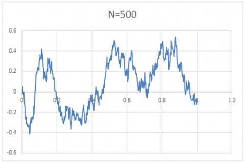
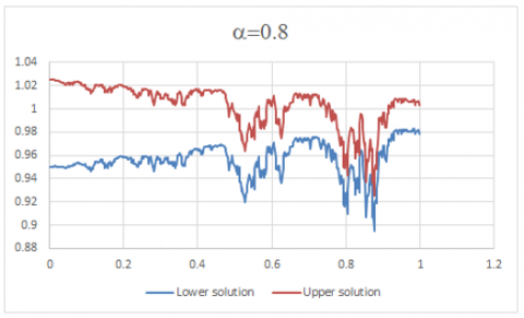
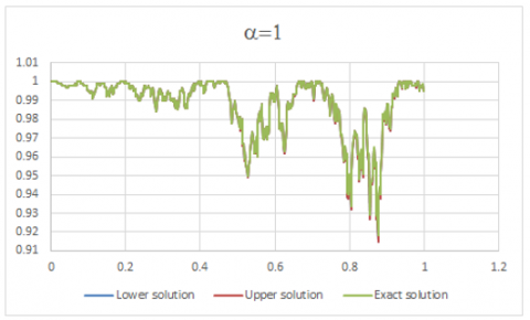
The VIM was used to solve this example and after three iterations, a highly accurate approximate solution were obtained. The simulation signal of the discretized Brownian motion is carried out over the interval [0,1] and the number of discretized Brownian motion (signal) are taken to be for N=100 and 500 (see Figure 1). So, taking the discretization step size to be h=1/N, and also for the upper and lower solutions with different a-levels equals to 0.2, 0.4, 0.6, 0.8 and 1 are shown in the Figures 2 and 3.
Figure 1. Discretized Brownian path with N=100 and 500 generations
Figure 2. Third iteration lower and upper solutions of Example 1 using VIM for different values of a-levels and discretized Brownian motion with signal processing number N=100
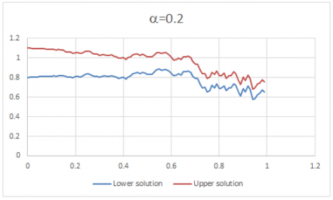
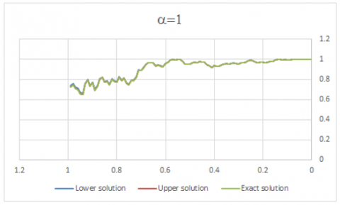
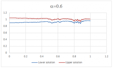
Figure 3. Third iteration lower and upper solutions of Example (4) using VIM for different values of a-levels and discretized Brownian motion with signal processing number N=500
Example (5): Consider the second order linear FRODEs:
$\frac{\mathrm{d}^2 \tilde{x}(t ; \omega)}{\mathrm{dt}^2}-\mathrm{W}_{\mathrm{t}}^2(\omega) \tilde{x}(\mathrm{t} ; \omega)=0, t \in[0,1]$
subject to the fuzzy initial conditions for all $\alpha \in[0,1]$:
$\tilde{x}(0)=[0.75+0.25 r, 1.125-0.125 r]$
in which the crisp or the exact solution (when a=1) is given by:
$x(t ; \omega)=\frac{1}{2}\left(e^{\omega t}+e^{-\omega t}\right)$
Therefore, using the VIM with N=100 and 500, where a $\in$ [0,1], getting:
$\tilde{x}_{m+1}(t ; \omega)=\tilde{x}_m(t ; \omega)+\int_0^t(s-t)\left(\frac{d^2 \tilde{x}_m(s ; \omega)}{d s^2}-W_s^2(\omega) \tilde{x}_m(s ; \omega)\right) d s$
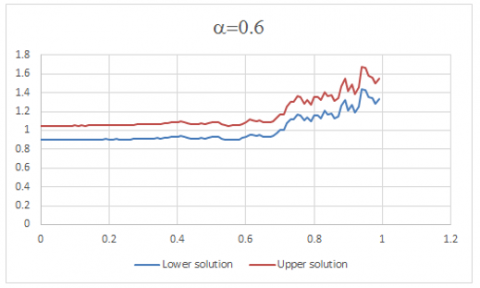
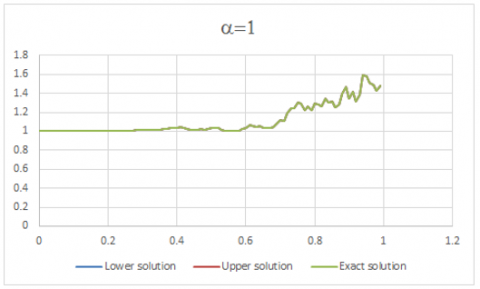
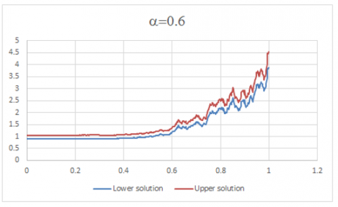
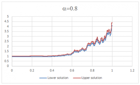
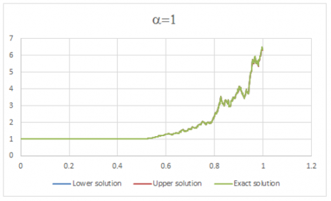
Similarly, the VIM was used to solve this example and after three iterations, a highly accurate approximate solution were obtained and the signal simulation of discretized Brownian motion is carried over the interval [0,1]. The number of discretized Brownian motion (signal) are taken to be for N=100 and 500 which are the same as those given in Figure 1. So, taking the discretization step size to be h=1/N, and also for the upper and lower solutions with different a-levels equals to 0.2, 0.4, 0.6, 0.8 and 1 are shown in the Figures 4 and 5.
Figure 4. Third iteration lower and upper solutions of Example (5) using VIM for different values of a-levels and discretized Brownian motion with signal processing number N=100
Figure 5. Third iteration lower and upper solutions of Example (5) using VIM for different values of a-levels and discretized Brownian motion with signal processing number N=500
The results derived from Examples (4) and (5) underscore the efficiency and reliability of the Variational Iteration Method (VIM) when applied to solving Fuzzy Random Ordinary Differential Equations (FRODEs). This finding can be seen as a generalization of the results obtained for solving crisp Random Ordinary Differential Equations (RODEs), specifically when α=1.
Concerning the temporal complexity of the proposed algorithm for resolving FRODEs, it should be noted that it could be considered computationally demanding depending on the number of random number generations. As the quantity of discretized Brownian motion along with the signal processing number escalates, a corresponding increase in computational time is observed.
[1] Zadeh, L.A. (1965). Fuzzy sets. Information and Control, 8(3): 338-353. https://doi.org/10.1016/S0019-9958(65)90241-X
[2] Friedman, M., Ma, M., Kandel, A. (1999). Numerical solutions of fuzzy differential and integral equations. Fuzzy Sets and Systems, 106(1): 35-48. https://doi.org/10.1016/S0165-0114(98)00355-8
[3] Abbasbandy, S., Viranloo, T.A. (2002). Numerical solutions of fuzzy differential equations by Taylor method. Computational Methods in Applied Mathematics, 2(2): 113-124. https://doi.org/10.2478/cmam-2002-0006
[4] Jafari, H., Saeidy, M., Baleanu, D. (2012). The variational iteration method for solving n-th order fuzzy differential equations. Central European Journal of Physics, 10: 76-85. https://doi.org/10.2478/s11534-011-0083-7
[5] Allahviranloo, T., Abbasbandy, S., Behzadi, S.S. (2014). Solving nonlinear fuzzy differential equations by using fuzzy variational iteration method. Soft Computing, 18: 2191-2200. https://doi.org/10.1007/s00500-013-1193-5
[6] Sadigh Behzadi, S. (2018). The use of fuzzy variational iteration method for solving second-order fuzzy Abel-Volterra integro-differential equations. International Journal of Industrial Mathematics, 10(2): 211-219.
[7] Fadhel, F.S., Sagban, H.M. (2021). Approximate solution of linear fuzzy initial value problems using modified variaional iteration method. Al-Nahrain Journal of Science, 24(4): 32-39. https://doi.org/10.22401/ANJS.24.4.05
[8] Han, X., Kloeden, P.E. (2017). Random Ordinary Differential Equations and Their Numerical Solution. Springer, Nature, Singapore. https://doi.org/10.1007/978-981-10-6265-0
[9] Cortés, J.C., Jódar, L., Villafuerte, L. (2007). Numerical solution of random differential equations: A mean square approach. Mathematical and Computer Modelling, 45(7-8): 757-765. https://doi.org/10.1016/j.mcm.2006.07.017
[10] Cortés, J.C., Jódar, L., Villafuerte, L., Company, R. (2011). Numerical solution of random differential models. Mathematical and Computer Modelling, 54(7-8): 1846-1851. https://doi.org/10.1016/j.mcm.2010.12.037
[11] Khudair, A.R., Ameen, A.A., Khalaf, S.L. (2011). Mean square solutions of second-order random differential equations by using variational iteration method. Applied Mathematical Sciences, 5(51): 2505-2519.
[12] Khudair, A.R., Ameen, A.A., Khalaf, S.L. (2011). Mean square solutions of second-order random differential equations by using Adomian decomposition method. Applied Mathematical Sciences, 5(51): 2521-2535.
[13] Khudair, A.R., Haddad, S.A.M., Khalaf, S.L. (2016). Improve the mean square solution of second-order random differential equations by using homotopy analysis method. British Journal of Mathematics & Computer Science, 16(5): 1-14.
[14] Tchier, F., Vetro, C., Vetro, F. (2017). Solution to random differential equations with boundary conditions. Electronic Journal of Differential Equation, 2017: 1-12.
[15] Abdulsahib, A.A., Fadhel, F.S., Abid, S.H. (2019). Modified approach for solving random ordinary differential equations. Journal of Theoretical and Applied Information Technology, 97(13): 3574-3584.
[16] Feng, Y. (1999). Mean-square integral and differential of fuzzy stochastic processes. Fuzzy Sets and Systems, 102(2): 271-280. https://doi.org/10.1016/S0165-0114(97)00119-X
[17] Malinowski, M. (2011). Peano type theorem for random fuzzy initial value problem. Discussiones Mathematicae, Differential Inclusions, Control and Optimization, 31(1): 5-22. https://doi.org/10.7151/dmdico.1125
[18] Vu, H., Dong, S.L., Hoa, V.N. (2014). Random fuzzy functional integro-differential equations under generalized Hukuhara differentiability. Journal of Intelligent & Fuzzy Systems, 27(3): 1491-1506. https://doi.org/10.3233/IFS-131116
[19] Khastan, A., Nieto, J.J., Rodriguez-Lopez, R. (2011). Variation of constant formula for first order fuzzy differential equations. Fuzzy Sets and Systems, 177(1): 20-33. https://doi.org/10.1016/j.fss.2011.02.020
[20] Park, J.Y., Jeong, J.U. (2013). On random fuzzy functional differential equations. Fuzzy Sets and Systems, 223: 89-99. https://doi.org/10.1016/j.fss.2013.01.013
[21] Kwakernaak, H. (1978). Fuzzy random variables—I. Definitions and theorems. Information Sciences, 15(1): 1-29. https://doi.org/10.1016/0020-0255(78)90019-1
[22] Puri, M.L., Ralescu, D.A. (1985). The concept of normality for fuzzy random variables. The Annals of Probability, 13(4): 1373-1379.
[23] Feng, Y. (2000). Fuzzy stochastic differential systems. Fuzzy sets and Systems, 115(3): 351-363. https://doi.org/10.1016/S0165-0114(98)00389-3
[24] Fei, W. (2007). Existence and uniqueness of solution for fuzzy random differential equations with non-Lipschitz coefficients. Information Sciences, 177(20): 4329-4337. https://doi.org/10.1016/j.ins.2007.03.004
[25] Malinowski, M.T. (2009). On random fuzzy differential equations. Fuzzy Sets and Systems, 160(21): 3152-3165. https://doi.org/10.1016/j.fss.2009.02.003
[26] Malinowski, M.T. (2012). Random fuzzy differential equations under generalized Lipschitz condition. Nonlinear Analysis: Real World Applications, 13(2): 860-881. https://doi.org/10.1016/j.nonrwa.2011.08.022
[27] Boswell, S.B., Taylor, M.S. (1987). A central limit theorem for fuzzy random variables. Fuzzy Sets and Systems, 24(3): 331-344. https://doi.org/10.1016/0165-0114(87)90031-5
[28] Arnold, L. (1974). Stochastic Differential Equations; Theory and Application. John-Wiley and Sons, Inc.
[29] Röble, A. (2003). Runge-Kutta methods for numerical solution of stochastic differential equations. Ph.D. Thesis. Department of Math, technology University, Germany.
[30] Arnold, L. (1998). Random Dynamical Systems. Springer, Berlin.
[31] Kloeden, P.E., Platen, E. (1992). Numerical Solutions of Stochastic Differential Equations. Springer, Berlin.
[32] Gr. Voskoglou, M. (2015). Use of the triangular fuzzy numbers for student assessment. American Journal of Applied Mathematics and Statistics, 3(4): 146-150. https://doi.org/10.12691/ajams-3-4-2
[33] Ghanbari, M. (2012). Solution of the first order linear fuzzy differential equations by some reliable methods. Journal of Fuzzy Set Valued Analysis, 2012: 20.
[34] Tapaswini, S., Chakraverty, S. (2014). New analytical method for solving n-th order fuzzy differential equations. Ann Fuzzy Math Inform, 8: 231-244.
[35] Tapaswini, S., Chakraverty, S., Allahviranloo, T. (2017). A new approach to nth order fuzzy differential equations. Computational Mathematics and Modeling, 28: 278-300. https://doi.org/10.1007/s10598-017-9364-3
[36] Chakraverty, S., Tapaswini, S., Behera, D. (2016). Fuzzy Differential Equations and Applications for Engineers and Scientists. Boca Raton, FL: CRC Press.
[37] Corliss, G.F. (1995). Guaranteed error bounds for ordinary differential equations. In Theory of Numerics in Ordinary and Partial Differential Equations (ed. M. Ainsworth, J. Levesley, W.A. Light and M. Marletta). Oxford: Oxford University Press.
[38] Jafari, H., Alipoor, A. (2011). A new method for calculating general Lagrange multiplier in the variational iteration method. Numerical Methods for Partial Differential Equations, 27(4): 996-1001. https://doi.org/10.1002/num.20567
[39] Wazwaz, A.M. (2010). The variational iteration method for solving linear and nonlinear Volterra integral and integro-differential equations. International Journal of Computer Mathematics, 87(5): 1131-1141. https://doi.org/10.1080/00207160903124967
[40] Odibat, Z. M. (2010). A study on the convergence of variational iteration method. Mathematical and Computer Modelling, 51(9-10): 1181-1192. https://doi.org/10.1016/j.mcm.2009.12.034