Priyanka Ramdass![]() | Gajendran Ganesan*
| Gajendran Ganesan*![]()
© 2023 IIETA. This article is published by IIETA and is licensed under the CC BY 4.0 license (http://creativecommons.org/licenses/by/4.0/).
OPEN ACCESS
The prevalence of heart disease, often exacerbated by unhealthy lifestyle choices, necessitates timely and accurate diagnosis—a task that can often be laborious for medical professionals. Over time, machine learning algorithms have demonstrated significant promise in facilitating efficacious predictions within healthcare settings. This study introduces a novel automatic classification model, Neighbourhood Component Analysis Optimized Multilayer Feed-Forward Neural Network (NCA-MLFFNN), designed to predict the onset of heart disease. The first phase of the proposed model employs Neighbourhood Component Analysis (NCA), a technique that aids in selecting the optimal features from the neighbourhood. Subsequently, a robust Multilayer Feedforward Neural Network (MLFFN) model is developed to train these selected features. A notable innovation in this work is the unique approach to data partitioning. Breaking away from the traditional practice of randomly dividing data into training and testing sets, the proposed model employs NCA for strategic data splitting. To enhance the precision of classification and minimize the misclassification rate, a backpropagation algorithm is employed. The study also includes a comparative analysis of various machine learning algorithms to gauge their performance. Experimental results suggest that the NCA-MLFFNN model outperforms other models, achieving an impressive accuracy of 96.03%. This paper, therefore, underscores the potential of NCA-MLFFNN as an effective tool in predicting heart disease and facilitating early intervention.
neighbourhood component analysis, multilayer feed forward neural network, backpropagation, Cleveland dataset
The heart, a pivotal organ in the human body, is responsible for pumping blood through an extensive network of vessels spanning approximately 60,000 miles. With an astounding 100,000 beats per day, it achieves forty million beats annually, culminating in nearly three billion beats over an average lifetime. The heart's functions are not limited to the oxygenation of the body and nutrient delivery to cells, but it also plays a crucial role in waste removal. Despite its significance, cardiovascular disease remains the leading cause of mortality globally, with the World Health Organisation (WHO) reporting that approximately 17.9 million people succumb to heart disease annually. As such, early prediction and intervention are critical in curtailing the mortality rate associated with heart disease.
Irregular heartbeats serve as a primary symptom of heart disease, necessitating the maintenance of various heart metrics, ranging from blood pressure to cholesterol levels. Although some of these metrics require professional evaluation, others can be monitored at home. A healthy heart offers resistance against major health issues and facilitates early detection of anomalies. Myocardial infarction, commonly known as a heart attack, is triggered when a region of the heart muscle is deprived of adequate blood supply. This is primarily attributed to coronary heart disease, although severe spasms or sudden contractions can also disrupt blood flow to the heart muscle.
Risk factors for heart disease often stem from detrimental behaviours, resulting in conditions such as obesity, hypertension, hyperglycaemia, and high cholesterol. Noteworthy symptoms of a heart attack in both men and women include chest discomfort, weakness, lightheadedness, fainting, pain or discomfort in one or both arms or shoulders, and shortness of breath. Additional symptoms may encompass unusual fatigue, nausea, or vomiting.
The exponential increase in medical data collection presents a formidable opportunity for medical practitioners to enhance their diagnostic capabilities. The remainder of this paper is structured as follows: Section 2 reviews related works, Section 3 details the proposed methodology, Section 4 engages in discussion, Section 5 presents an analysis of the results, and Section 6 offers a conclusion and outlines potential avenues for future research.
This section delves into various machine learning techniques and models harnessed by multiple researchers to predict heart disease, focusing primarily on the Cleveland dataset.
Ramalingam et al. [1] conducted a survey on a host of machine learning algorithms, such as Naive Bayes (NB), Support Vector Machine (SVM), K–Nearest Neighbour (KNN), Decision Tree (DT), Random Forest (RF), Neural Network (NN), and Logistic Regression (LR), that have been employed extensively in recent years for heart disease prediction. According to their findings, SVM significantly outperformed other techniques such as NB, KNN, DT, and RF in terms of accuracy [1].
A similar survey was undertaken by Limbitote et al. [2], who compared various data mining techniques such as NB, SVM, KNN, DT, RF, NN, and LR. Their goal was to identify the most suitable machine learning technique for early prediction of heart disease among the general population.
Alic et al. [3] leveraged machine learning techniques such as Artificial Neural Networks (ANN) and Bayesian Networks (BN) to classify diabetes and cardiovascular disease. Furthermore, they incorporated the Levenberg-Marquardt learning algorithm of a multilayer feed-forward neural network into the ANN technique, concluding that this combination yielded more reliable statistics in classifying diabetes and heart disease diagnoses.
In another study, Maheshwari and Jasmine [4] applied a combined approach of logistic regression and neural network-based models. An ANN was trained using risk factors derived from logistic regression for testing heart disease among individuals. The proposed model was divided into two parts: the first part identified crucial risk factors based on the p-value, which provided necessary codes for each attribute, and the second part partitioned the dataset into training and testing sets. A neural network was then constructed for both training and testing.
Chen et al. [5] proposed a model that implemented the Learning Vector Quantization Algorithm, an ANN learning technique. Performance was evaluated using the ROC curve, Sensitivity, Accuracy, and Specificity.
Sonawane and Patil [6] trained an entire network using the Vector Quantization Algorithm via random order incremental training. Meanwhile, Das et al. [7] conducted an experimental study on the Cleveland dataset using neural network ensembles, incorporating SAS-related software 91.3 for prediction.
Gavhane et al. [8] employed ANN and the Multilayer Perceptron algorithm to train, test, and validate the Cleveland dataset for heart disease prediction, finding that the MLP provided reasonable accuracy.
While these existing models demonstrated satisfactory performance rates, the model proposed in this paper introduces an efficient and reliable Neighbourhood Component Analysis (NCA) technique, aiming to outperform existing models.
The motivation behind creating a multilayer feedforward neural network is its superior capability to handle highly non-linear data. This work utilizes the non-linear Cleveland dataset and employs the sigmoid activation function to learn the non-linearity between the data, thereby approximating the desired output for any given input.
In this section, we emphasize the significance of widely used machine learning technique called Multilayer Feed Forward Neural Network. Also, all its variants and derivatives are discussed in brief.
3.1 Artificial neural network
Artificial Neural Network is a machine learning paradigm which is a “representation” and “reflection” of functioning of human brain. Neural Network is an art of constructing a computer program which learns from observational data. In 1958, Franklin Rosenblatt invented a simple binary classifier model called Perceptron. Perceptron is a building block of an artificial neural network. Perceptron is the most basic form of neural network comprised of single neuron. Multilayer Perceptron (MLP) is a generalized neural network model consists of four main parameters namely input values, weight and bias and activation function. Perceptron takes real values as its inputs.
3.2 Multilayer feed forward neural network
The fully connected artificial neural network is called multilayer feed forward neural network (MLFFN) [9]. Generalization of a single layer perceptron is known as multilayer perceptron (MLP) or multilayer feed forward neural network. MLFFN has multiple hidden nodes. In this type of network, all the input vector passes to the hidden layer and then to output layer. Each node in a single layer is connected to every other node in the next layer. All the internal calculation and extraction take place in the hidden layer.
The MLFFNN takes the input vector along with some random weights and bias and that representation is called as linear combination. Then, the linear combination or the weighed sum is passed to the transfer function or the sigmoid activation function. Sigmoid activation function has the ability to transfer the real valued data to lie between “0” and “1”. Sigmoid function has an advantage of predicting the probability of a binary data. After processing the linear combination, the output from the hidden layer passes to the output layer. Hence, MLFFN reconstruct each input vector into desired output vector with appropriate weight components.
3.3 Mathematical formulation MLFFNN
Let $X \subset[0,1]^m$ is a real valued input vectors whose components are defined as $\bar{x}=\left(x_1, x_2, \ldots x_m\right)$. Let $Y \subset$ $[0,1]^m$ is an output vectors whose components are defined as $\overline{o o}=\left(o o_1, o o_2, \ldots o o_m\right)$.
Mathematical formation of MLFFN [10] with single hidden layer is defined by function $\mathrm{N}: \mathrm{X} \rightarrow \mathrm{Y}$ such that it converts input vector into desired output vector over the subsequent composition.
Input to the $j^{\text {th }}$ hidden neuron $i h_j$ is given by the linear combination input vector $\bar{x}_l$ and weight vector.
i.e.,$i h_j=\sum_{i=1}^{m+1} w i h_{j i} x_i$ (1)
where, $\left(w{i h_{j 1}}, w i h_{j 2} \ldots w i h_{j m}, w i h_{j(m+1)}\right) \in R^{m+1}$ defines the weight vector between the input layer and $j^{\text {th }}$ hidden neuron for all $j$ and $x_{m+l}$ is bias term and is equal to one.
Output to jth hidden neuron ohj is computed by the activated function for studying non-linearity on the input vectors.
i.e., $\quad o h_j=\frac{1}{1+e^{-i h_j}}$ (2)
Input to the kth hidden neuron iok is represented by the linear combination of vector ohj and weight vector.
i.e., $\quad i o_k=\sum_{j=1}^{h+1} w h o_{k j} o h_j$ (3)
where, $\left(w h o_{k 1}, w h o_{k 2}, \ldots w h o_{k h}, w h o_{k(h+1)}\right) \in R^{h+1}$ defines the weight vector the hidden layer and kth output neuron for all k, h is number of hidden output neuron for all k, h is number of hidden neurons and ohh+1 is bias term and is equal to one. Output to kth output neuron ook is computed by the activated function for studying non-linearity on the input vectors.
i.e., $\quad o o_k=\frac{1}{1+e^{-i o_k}}$ (4)
It can be expressed as $N\left(\mathrm{x}^{\mathrm{P}}\right)=o o_k$, where, $o o_k$ represents the final output $k^{\text {th }}$ component.
Figure 1. Multilayer feed forward neural
Figure 1 shows the typical multilayer Feedforward neural network. Generally, in feedforward propagation all the input vector directly moves to hidden layers and then to the output layer without forming any loops or cycles inside the network. Finally, the output which comes out of the output layer is considered as a predicted value. Mostly, all predicted value may not be equal to the actual value. If the predicted value does not match the actual value, there is possibility of misclassification or loss function. In order to retrieve the error, we employ a most prominent machine learning algorithm called backpropagation algorithm. BPN is leading algorithm in reducing the error rate. It reduces the error rate by computing the derivate of the loss function with respect to weight components in the input layer. weights are adjusted after one cycle. This process is Feedback propagation.
3.4 Back propagation
In 1974, Werbos and in 1985, Parker introduced an algorithm called backpropagation (BPN) algorithm. And in 1986, it was further developed by Rumelhart [11]. BPN is a machine learning algorithm used to minimize the loss function while training a multilayer feed forward neural network. It is a process of updating all the weight components with respect to the error rate. It is an algorithm which backpropagates all the error from output node to hidden node and then to input node.
Backpropagation works under these following steps.
3.5 Gradient descent and its variants
In 1847 “Augustin -Louis Cauchy” discovered an algorithm called Gradient descent algorithm. It is popularly known as steepest descent. It is an iterative optimization method which minimize the cost function for finding the local minimum of a function. It is the first order optimization algorithm used to train neural network model. We use batch gradient descent algorithm train our MLFFFNN. This algorithm takes each training data into account in every iteration. It takes the average of gradient of overall training samples and the mean gradient is used to update. The model updates its weight parameter after every epoch.
3.5.1 Learning rate
Learning rate is the hyper parameter which controls the weight with respect to the loss function. A smaller learning rate needs additional training epoch. Therefore, learning rate basically plays a significant role in controlling the weight parameter. Any smaller changes made to the weight in each iteration which makes the model converge slowly to the global minimum loss.
3.5.2 Error correction
Error is the measure of loss function between the actual value and predicted value. It basically affects the performance of the model and it can be calculated by the following formula:
$E(\bar{W})=\frac{1}{2} \sum_{p=1}^p \sum_{k=1}^n\left(e_k^p\right)^2$ (5)
where, $e_k^p=d_k^p-o o_k^p, d_k^p$=actual output, $o o_k^p$=predicted output.
4.1 Dataset description
For this experimental study, the Cleveland database is used for classification. The dataset is collected from University of California Irvine (UCI,1990) a machine learning repository. The data is structured with 303 instances. It is a labelled data. The labelled feature represents the presence and absence of heart disease. The labelled data has 165 heart disease patients and 138 non- heart disease patients. The description of the Cleveland data is given in Table 1.
4.2 Data pre-processing
The data normalization is highly essential part to find trends in the data by comparing the features of data points. Normalization has the greatest tendency to compare the features of data to one another. When an algorithm tries to predict the desired output, the algorithm correlates the data points all along the component with larger scale will entirely monopolize the component with smaller scale. The main goal of normalization approach is to assemble every component into equivalent scale with the intention that every component or feature is important. It is the process of cleaning the data where every feature with minimum value gets transformed into zero, and every feature with maximum value get transformed into one. Min-Max Normalization can be calculated mathematically using the below formula:
$x^{\prime}=a+\frac{x-\min (x)(b-a)}{\max (x)-\min (x)}$ (6)
The normalized data is highly non- linear and it is visualized in the Figure 2.
Table 1. Description of Cleveland data
|
S. No. |
Attributes |
Description |
|
1 |
Age |
Age in years |
|
2 |
Gender |
Gender type |
|
3 |
Cp |
Chest pain level |
|
4 |
Trestbps |
Blood pressure in mm Hg |
|
5 |
Chol |
Level of serum cholesterol in mg/dl |
|
6 |
Fbs |
Level of fasting blood sugar ≥120 mg/dl |
|
7 |
Rest ecg |
Level of resting electro cardio graphic |
|
8 |
Thalach |
Maximum heart rate |
|
9 |
Exang |
Exercise induced |
|
10 |
Old peak |
ST level at exercise, exercise relative to rest |
|
11 |
Slope |
Level of the peak exercise in ST- segment |
|
12 |
Ca |
Flourosopy vessel level |
|
13 |
Thal |
Heart status |
|
14 |
Diagnosis of Heart disease |
Class I=Healthy, Class II=Sick |
Figure 2. Distribution of data
4.3 Nearest neighbour component analysis
In this paper, the optimal clusters are obtained by using nearest neighbour component analysis (NCA). NCA is a supervised machine learning algorithm [12], it is a generalized idea of a set of points circumscribed to a given point. NCA is a nonparametric classification model without any consideration of the shape or the distribution of the classes also the boundaries between them. Distance metric finds the closest data points as it reduces the dimensionality of the data thereby reducing the storage and search time as well. In a system, a neighbourhood point is always a non-empty set. Most of the machine learning algorithms incorporate distance metric algorithms in it is models to compute the affinity between the data points.
4.4 Cluster analysis
Cluster analysis plays a major role in data mining techniques. It is a method of decomposing the high dimensional data set X into smaller subsets. Several clustering algorithms K-means clustering, hierarchical, Self-organizing Maps and EM algorithms can be used to map its representatives. In this paper, Nearest Neighbourhood component analyses are used to make cluster algorithms to find a group of data based on the similarity of the features. The quality of the cluster will enhance the performance of the model [13]. Now, the paradigm of all points connecting its nearest neighbour is stated in the following.
Given collection of data points $X=\left\{\overline{x_l}: \overline{x_l}=\left(x_{i 1}, x_{i 2}, \ldots, x_{i n}\right), i=1,2, \ldots, p\right\}$ where $x_{i j} \in[0,1]$ are labelled as class I and class II. A Euclidean distance between two real-valued vectors $\overline{\mathrm{x}_1}, \overline{\mathrm{x}_{\mathrm{j}}} \in \mathrm{X}$ is expressed as:
$d\left(\bar{x}_l, \bar{x}_J\right)=\left|\bar{x}_l-\bar{x}_J\right|^2$ (7)
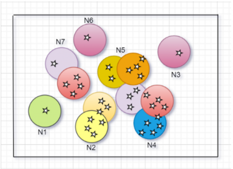
A neighbourhood of a point $\bar{x} \in X$ is a set $N(\bar{x})$ consisting of some points $\bar{x}_l \in X$ such that $d\left(\bar{x}, \bar{x}_l\right) \leq r$ where the real number $r$ is called the radius of $N(\bar{x})$. For fixed $r, X$ consists finite number of clusters $N_i(\bar{x}), i=1,2, \ldots, l$ as shown in the Figure 3.
Figure 3. Categorization of Ni(x)
Classification of learning set L and testing set T based on categorization of $N_i(\bar{x})$ are given as follows:
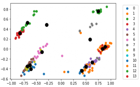
The probability of collecting the neighbour decreases as the distance between the points increases. Eventually, the data with neighbours are taken to test the data. NCA performed consistently on training data, and the test data was at top of the line. Reverting these following steps until we gain similar centroids. In such a way optimal clusters are formed as shown in the Figure 4.
Figure 4. Optimal clusters formed by NCA
The performance of ANN was constructed by Multilayer Feed Forward neural network. In MLFFN, any number of hidden layers can be added as per requirement. In the proposed model, only one hidden layer with nine neurons is used in MLFFN for which the MLFFN contributes the best results. Based on the proposed method, 75% of 303 data are used for training and the remaining 25% are used for testing. This model was trained under the combination of nearest neighbour algorithm-based multilayer perceptron. To determine the efficiency of the classification model with the best features selection we split the dataset into two distinct divisions. Firstly, the training set comprised 227 instances with 13 featured samples and one output label and the testing dataset consist of 76 instances. The decomposition of a 303×13 matrix is not determined randomly. Preferably, pretty proper data are collected for training the model by the NCA method. Ultimately, the quality and efficiency of the model will be higher. Each point in a training set is considered as its neighbour but with contrasting probabilities. The intersection of two point is treated to be zero.
The main goal of proposing a clustering algorithm is considering its optimal neighbour is to collect all possible numbers of data points to put in a training set. Instead of taking all the training data points in a random ratio here, our proposed methodology takes the data points which has the greatest impact as a result it improves the efficiency of the model.
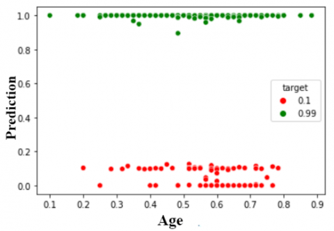
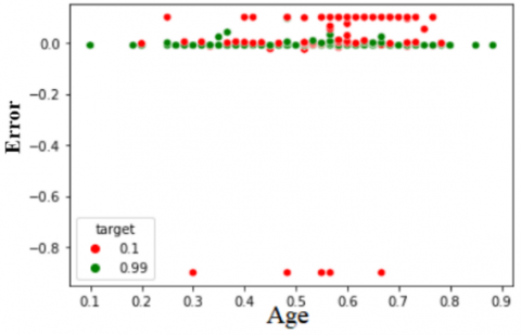
Figure 5 and Figure 6 show the individual contribution of the component such as age to predict the presence of heart disease through the proposed NCA-MLFFN technique.
In Figure 5, the attribute age is labelled on the x-axis and predicted values are labelled on y-axis. The proposed model plotted the healthy patient at the bottom and the heart disease patients at the top of the figure. Also, Figure 6 shows the performance of the developed NCA-MLFFN model classifying heart disease with its minimum loss function is shown.
Cleveland heart disease dataset is highly non-linear in nature as shown in Figure 2. Many researchers [4] have tried to classify Cleveland heart disease dataset. Even though the paper [4] had find the important risk factors on the p-value which gives the necessary codes for every attribute, accuracy produced by is 84% whereas proposed model produces the accuracy 97%. In the study [5], although measures the distance metric between the data point, the proposed model learning vector quantization produced its best accuracy of about 80% in the Learning Vector Quantization Algorithm, proposed model nearest neighbourhood is used to make cluster to find the groups of data based on the similarity of the features which produce the accuracy of 97%. In the study [6], the number of neurons in the hidden layer can be increased or decreased based on the error obtained. The performance of the system was improved by varying the epochs and the number of neurons. Eventually, the model in the study [6] obtained an accuracy of about 85.55% and Florence et al. [14], initially used three neurons in the hidden layer and it can be increased up to thirteen neurons whereas the proposed model uses nine fixed hidden neurons based on the method of the density of the learning data.
Figure 5. Distribution of age and prediction
Figure 6. Distribution of age and error
For the evaluation process, confusion matrix, accuracy score, Precision, Sensitivity and Specificity are used. Confusion Matrix is a matrix contains actual values and the predicted values and it is denoted by True Positive (TP) and True Negative (TN). It is a table like structure consist of four distinct sections. The first section contains True positive rate in which the predicted values correctly match to the actual value i.e., it identifies sick as sick. The second and third section has false positive rate (FP) in which predicted value does not match the actual value, it is also known as type I error and type II error. The fourth section has True Negative (TN) in which negative value is correctly identified as negative. The confusion matrix is shown in Tables 2, 3 and 4 in which P is positive, N is negative, TP is True Positive, FN is False Negative, FP is False Positive and TN is True Negative. Accuracy score is used to check how well the model is performed.
Accuracy score is used to check how well the model is performed.
Accuracy $=\frac{\mathrm{TP}+\mathrm{TN}}{(\mathrm{TP}+\mathrm{TN}+\mathrm{FP}+\mathrm{FN})} \times 100$ (8)
Sensitivity is a measure of True Positive rate.
Sensitivity $=\frac{T P}{(T P+F N)} \times 100$ (9)
Specificity is a measure of True Negative rate.
Specificity $=\frac{T N}{(T N+F P)} \times 100$ (10)
Precision is a measure of how many Positive classes are predicted correctly.
Precision $=\frac{T P}{(T P+F P) \times 100} \times 100$ (11)
Result of proposed system to predict heart disease is partitioned into two sections. First section of the confusion matrix asses the efficiency while training and building a model as shown in Table 2.
Table 2. Confusion matrix on training data
|
Actual/Predicted |
P |
N |
Total |
|
T |
109 |
112 |
221 |
|
F |
1 |
5 |
6 |
|
Total |
110 |
117 |
227 |
Second section of a confusion matrix reveals the performance of proposed model has been effective while integrating MLFFN with NCA as shown in Table 3.
Table 3. Confusion matrix on testing data
|
Actual/Predicted |
P |
N |
Total |
|
T |
4 |
46 |
70 |
|
F |
0 |
6 |
6 |
|
Total |
24 |
52 |
76 |
Evaluation of True positive rate and True negative rate of overall dataset using confusion matrix are shown in Table 4.
Table 4. Confusion matrix of predicted outcomes
|
Actual/Predicted |
P |
N |
Total |
|
T |
133 |
158 |
291 |
|
F |
7 |
5 |
12 |
|
Total |
140 |
163 |
303 |
Table 5 delivers the overall prediction performances while training and testing a model.
Table 5. Classification assessment
|
Data |
Accuracy |
Sensitivity |
Specificity |
Precision |
|
Training |
97.35% |
95.61% |
99.11% |
99.09% |
|
Testing |
92% |
80% |
100% |
100% |
Proposed system is compared with other classification model to assess the potency of the introduced system as shown in Table 6.
Table 6. Comparative analysis with existing model
|
References |
Classifiers |
Accuracy |
|
Mohan et al. [15] |
Hybrid random forest with a linear model |
87.98% |
|
Lakshmanarao et al. [16] |
Random Forest |
91.3% |
|
Kishore et al. [17] |
Recurrent Neural System |
92% |
|
Florence et al. [14] |
Back propagation algorithm |
95% |
Nevertheless, accuracy is the significant metric to confirm the efficiency of a method. In that sense, the proposed system shows high accuracy rate of 96.03% than other conventional studies as shown in Table 7.
Table 7. Performance of proposed model
|
Proposed Model |
Accuracy |
Sensitivity |
Specificity |
Precision |
|
NCA-MLFFN |
96.03% |
96.37% |
95.75% |
95% |
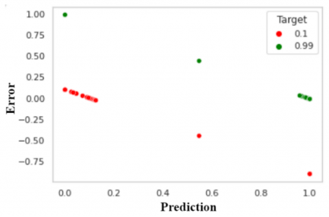
Figure 7 represents the performance of MLFFNNN model. It typically shows the difference between the predicted values and the error components occurred during testing the model. The model convergence at 114th epoch. Analysis of performance plot recorded a significantly lower error rate in comparison to other common classifiers.
Figure 7. Performance of the proposed model
The proposed model, which employs a nearest neighborhood search for training a multilayer feed forward neural network, demonstrates superior accuracy compared to other methods. Initial efforts were undertaken to pre-process the dataset, mitigating the risk of overfitting during the model's training phase. The proposed approach leverages a Neighbourhood selection technique to select optimal features for learning, thereby enhancing the model's generalization. The selected features were subsequently trained using a multilayer feedforward neural network (MLFFN).
The MLFFN was designed with a single hidden layer equipped with nine neurons. The model's efficiency was determined by the error rate obtained using the backpropagation algorithm. It is noteworthy that approximately 75% of the data was allocated for learning, while the remaining 25% was utilized for testing the model.
The model's performance was evaluated using various metrics such as Sensitivity, Specificity, and Precision, validated using a confusion matrix. The proposed algorithm ultimately achieved an impressive accuracy of approximately 96.03%.
In future works, the proposed model's performance may be enhanced through precise calibration of parameters for the same Cleveland heart disease data or by employing various distinct methodologies. The implementation of these modifications could potentially bolster the predictive power and overall performance of the model. Hence, the research opens avenues for further exploration and refinement of this model.
|
ANN |
Artificial Neural Network |
|
MLP |
Multilayer Perceptron |
|
MLFFNN |
Multilayer Feed Forward Neural Network |
|
BPN |
Back Propagation |
|
NCA |
Neighbour Component Analysis |
|
TP |
True Positive |
|
TN |
True Negative |
|
FP |
False Positive |
|
FN |
False Negative |
[1] Ramalingam. V.V., Dandapath, A., Raja, M.K. (2018). Heart disease prediction using machine learning techniques: A survey. International Journal of Engineering and Technology, 2112(1): 684-687. https://doi.org/10.14419/ijet.v7i2.8.10557
[2] Limbitote, M., Damkondwar, K., Mahajan, D., Patil, P. (2020). A survey on prediction techniques of heart disease using machine learning. International Journal of Engineering Research and Technology (IJERT), 9(6): 22780181. https://doi.org/10.17577/IJERTV9IS060298
[3] Alic, B., Gurbeta, L., Badnjevic, A. (2017). Machine learning techniques for classification of diabetes and cardiovascular diseases. Mediterranean Conference on Embedded Computing (MECO), pp. 1-4. https://doi.org/10.1109/ MECO.2017.7977152
[4] Maheswari, K.U., Jasmine, J. (2017). Neural network based heart disease prediction. International Journal of Engineering Research and Technology (IJERT), 5(17): 1-4. https://doi.org/10.17577/IJERTCONV5IS17019
[5] Chen, A.H., Huang, S.Y., Hong, P.S., Cheng, C.H., Lin, E.J. (2011). HDPS: Heart disease prediction system. In 2011 Computing in Cardiology, pp. 557-560.
[6] Sonawane, J.S., Patil, D.R. (2014). Prediction of heart disease using learning vector quantization algorithm. In 2014 Conference on IT in Business, Industry and Government (CSIBIG), Indore, India, pp. 1-5. https://doi.org/10.1109/CSIBIG.2014.7056973
[7] Das, R., Turkoglu, I., Sengur, A. (2009). Effective diagnosis of heart disease through neural networks ensembles. Expert Systems with Applications, 36(4): 7675-7680. https://doi.org/10.1016/j.eswa.2008.09.013
[8] Gavhane, A., Kokkula, G., Pandya, I., Devadkar, K. (2018). Prediction of heart disease using machine learning. In 2018 Second International Conference on Electronics, Communication and Aerospace Technology (ICECA), pp. 1275-1278. https://doi.org/10.1109/ICECA.2018.8474922
[9] Yan, H. (2006). A multilayer perceptron-based medical decision support system for heart disease diagnosis. Expert Systems with Application, 30(2): 272-281. https://doi.org/10.1016/j.eswa.2005.07.022
[10] Gajendran, G., Vasanthi, K. (2019). Multilayer feedforward neural networks with backpropagation model on immunotherapy dataset. AIP Conference Proceedings, 2112(1): 020102. https://doi.org/10.1063/1.5112287
[11] Li, J., Cheng, J. H., Shi, J.Y., Huang, F. (2012). Brief introduction of back propagation (BP) neural network algorithm and its improvement. Advances in Computer Science and Information Engineering, 2: 553-558. https://doi.org/10.1007/978-3-642-30223-7
[12] Samuel, O.W. (2020). A new technique for the prediction of heart failure risk driven by hierarchical Neighbourhood component-based learning and adaptive multi-layer networks. Future Generation Computer Systems, 1(110): 781-794. https://doi.org/10.1016/j.future.2019.10.034
[13] Gárate-Escamila, A.K., El Hassani, A.H., Andrès, E. (2020). Classification models for heart disease prediction using feature selection and PCA. Informatics in Medicine Unlocked, 19: 100330. https://doi.org/10.1016/j.imu.2020.100330
[14] Florence, S., Amma, N.B., Annapoorani, G., Malathi, K. (2014). Predicting the risk of heart attacks using neural network and decision tree. International Journal of Innovative Research in Computer and Communication Engineering, 2(11): 7025-7030.
[15] Mohan, S.C., Thirumalai., G, Srivastava. (2019). Effective heart disease prediction using hybrid machine learning techniques. IEEE Access, 7: 81542-81554. https://doi.org/10.1109/ACCESS.2019.2923707
[16] Lakshmanarao, A., Swathi, Y., Sundareswar, P.S.S. (2019). Machine learning techniques for heart disease prediction. International Journal of Scientific & Technology Research, 8(11): 374-377.
[17] Kishore, A., Kumar, A., Singh, K., Punia, M., Hambir, Y. (2018). Heart attack prediction using deep learning. International Research Journal of Engineering and Technology (IRJET), 5(4): 4420-4423.