Samira Faisal Abushilah*![]() | Rajaa Hasan Abbas
| Rajaa Hasan Abbas![]()
© 2023 IIETA. This article is published by IIETA and is licensed under the CC BY 4.0 license (http://creativecommons.org/licenses/by/4.0/).
OPEN ACCESS
Clustering, a pivotal technique in statistics, enables the summarisation of data sets through the identification of related object groups. A prevalent question in clustering literature pertains to the precise number of partitions present within a data set. An array of clustering methods and indices has been proposed to discern the optimal number of clusters within a data set, each following its own set of rules. However, none of these methods universally excel in capturing the true components across all types of data structures. Particularly, they tend to grapple with uniquely shaped data sets or instances where objects from different groups are in close proximity. In this study, the performance of several clustering methods (Single Linkage, Complete Linkage, Average Linkage, Centroid Linkage, Ward.2D Linkage, Median Linkage) is evaluated in conjunction with different internal validity indices (KL, CH, Sil, Gap). This evaluation utilises simulated data, encompassing varied models, sample sizes, and distance measures, and is conducted using R software 3.1. Furthermore, several external indices (Rand, F-M, Purity) are employed to ascertain the degree of agreement between the true clusters of data points and the partitions computed through the clustering methods.
clusters, linkage clustering methods, internal indices, external scores
Clustering is a common technique in statistics, which is addressed in many disciplines such as image analysis [1], machine learning [2], bioinformatics [3], pattern recognition [4], and data mining [5]. There are many available algorithms which attempt to select the optimal number of clusters in terms of their own rules; however, with a high performance no one capture the true clusters of all types of data structure [6]. In other words, clustering is the process of grouping items into groups (clusters) such that objects in the same cluster are more similar than those in other clusters. One of the well-known clustering algorithms is called hierarchical clustering which is a common methodology in statistics (more details can be found in studies [7] and [8]. There are two different hierarchical clustering approaches: agglomerative and divisive hierarchical methods. Our main interest in this paper is the agglomerative hierarchical method, which starts with the distance matrix and each object being in a separate cluster, then in each agglomeration step, we merge the closest clusters. Our goal is to select the clustering algorithms which have the ability to capture the true clusters with high performance under different models and different sample sizes, where this technique could use to evaluate the performance of the new suggested approaches. Therefore, in this paper, different models and different distance measures are used to evaluate the performance of some clustering methods (single linkage, complete linkage, average linkage, centroid linkage, ward.2D linkage, median linkage) under different validity indices (KL, CH, Sil, Gap), different simulated data and different sample sizes using R software 3.1. Also, some external indices (Rand, F-M, Purity) will be used to get the rate of agreement between the true clusters of the data points and the partitions that we have computed using clustering methods. The results of all models show that the clustering method average linkage results with CH index match the true clusters about more that 90% with different distance measure and different sample sizes. There are three main possible linkage procedures in hierarchical clustering which are: single linkage (closest neighbour), complete linkage (furthest-neighbour) and average linkage. When we merge two clusters, we have to update the distance matrix depending on the choice of linkage method. For example, suppose we have a data set, {x1, x2…x5}, and assume the distance between the observations x2 and x4, d24, is the smallest. Thus, x2 and x4 are merged together in the first agglomeration step, and we denote this new cluster with x6 [9]. The distance between x6 and x1 is
$\mathrm{d}_{61}=\min \left\{\mathrm{d}_{21}, \mathrm{~d}_{41}\right\}$ (1)
and in the same way distances between the new cluster and other data points are updated. If we use the complete linkage or average linkage, the distance between x6 and x1 will be calculated respectively as follows [10]:
$\mathrm{d}_{61}=\max \left\{\mathrm{d}_{21}, \mathrm{~d}_{41}\right\}$ or $\frac{1}{2}\left(\mathrm{~d}_{21}+\mathrm{d}_{41}\right)$ (2)
Simulated Data: For illustrative purposes, two-component data from N(μ, σ2) in R2 is generated and shown in Table 1, where each component includes three observations. The tree for the simulated data is hierarchically build using Euclidean distances with average linkage, where the Euclidean distance is given by:
$d(x, y)=\sqrt{\sum_{j=1}^d\left(x_j-y_j\right)^2}$ (3)
The Euclidean distance matrix for the simulated data in Table 1 is computed and is shown in Table 2, and objects is clustered hierarchically using the stats package (R Core Team, 2017) in R. The dendrogram corresponding to the generated data is given in Figure 1. Blue labels for the internal nodes represent the agglomeration order, and internal nodes are labelled starting from n + 1, where n is the number of objects in the data, so n = 9, and the possible clustering schemes for this dendrogram are given in Table 3.
Table 1. Generated data from N(μ, σ2) in R2
|
Index |
Component |
1st Dimension |
2nd Dimension |
|
1 |
1 |
0.356 |
1.637 |
|
2 |
1 |
0.826 |
1.912 |
|
3 |
1 |
0.739 |
0.244 |
|
4 |
2 |
3.138 |
3.343 |
|
5 |
2 |
2.049 |
1.721 |
|
6 |
2 |
2.163 |
0.726 |
|
7 |
3 |
3.998 |
5.403 |
|
8 |
3 |
4.911 |
4.971 |
|
9 |
3 |
6.320 |
4.213 |
|
|
1 |
2 |
3 |
4 |
5 |
6 |
7 |
8 |
|
2 |
0.545 |
|
|
|
|
|
|
|
|
3 |
1.444 |
1.670 |
|
|
|
|
|
|
|
4 |
3.264 |
2.719 |
3.919 |
|
|
|
|
|
|
5 |
1.695 |
1.238 |
1.974 |
1.954 |
|
|
|
|
|
6 |
2.024 |
1.787 |
1.503 |
2.793 |
1.002 |
|
|
|
|
7 |
5.239 |
4.717 |
6.102 |
2.232 |
4.166 |
5.024 |
|
|
|
8 |
5.645 |
5.103 |
6.304 |
2.407 |
4.330 |
5.057 |
1010 |
|
|
9 |
6.497 |
5.956 |
6.848 |
3.299 |
4.945 |
5.426 |
2.609 |
1.6 |
|
q |
Dj where j $\in${1, 2, …, q} |
|
1 |
{1,2,3,4,5,6,7,8,9} |
|
2 |
{1,2,3,5,6}, {4,7,8,9} |
|
3 |
{1,2,3,5,6},{4}, {7,8,9} |
|
4 |
{1,2,3,5,6},{4}, {7,8},{9} |
|
5 |
{1,2,3},{4}, {5,6}, {7,8},{9} |
|
6 |
{1,2},{3},{4}, {5,6}, {7,8},{9} |
|
7 |
{1,2},{3},{4},{5},{6},{7},{8},{9} |
|
8 |
{1},{2},{3},{4},{5},{6},{7},{8},{9} |
Figure 1. The dendrogram of the data in Table 1
After a dendrogram is building, it is not easy to know where to cut the tree in order to determine how many clusters we have. Thus, we need some algorithms which help us to select a partition represents the data better. To address this question, in the literature some indices which is called internal cluster validity indices are proposed. In the next section, we will discuss these indices in detail.
Cluster validity indices can be divided into two types: internal indices and external scores. Internal indices are used to choose the best partitioning after applying the clustering algorithm. While, the external scores can be used to measure the agreement between the true partition and the results of clustering if the true partition of the data is known [11]. In the following sections we will discuss these indices in detail.
2.1 Internal indices
In the literature, there are many internal indices, so we pick four different internal indices from the most commonly referenced indices: Calinski and Harabasz index (CH index) [12], Silhouette index (Sil index) [13], Krzanowski and Lai index (KL index) [14] and Gap index [15]. All these internal indices are available in the NbClust package [16] in R. Internal index calculations are based on two quantities which are between-cluster sum of squares (BSS) and within-cluster sum of squares (WSS). So, we have to define BSS and WSS with some notation which are used in the discussion of various indices. We define:
$c_j=\frac{1}{m_j} \sum_{i \in C_J} x_i$ (4)
Depending on the above notations, BSS and WSS are defined by the following equations:
$B S S(q)=\sum_{j=1}^q m_j\left(c_j-\bar{x}\right)\left(c_j-\bar{x}\right)^T$ (5)
$\operatorname{WSS}(q)=\sum_{j=1}^q \sum_{i \in C_j}\left(x_j-c_j\right)\left(x_j-c_j\right)^T$ (6)
The CH index (Calinski and Harabasz index) was proposed in the study [12] and this index is defined by:
$C H I(q)=\frac{\operatorname{tr}(B S S(q) /(q-1)}{\operatorname{tr}(W S S(q) /(m-q)}, q>1$ (7)
If we cluster the similar objects together, BSS(q) will be high, and WSS(q) will be small and we can take the proportion of BSS(q) and WSS(q). Then, the optimal number of clusters is the value of q which maximizes CHI, because CHI will take the maximum value when large distances will be occur between clusters.
The KL index (Krzanowski and Lai index) was suggested in the study [15] and this index is given by:
$K L I(q)=\left|\frac{D I F F(q)}{D I F F(q+1)}\right|, q \geq 2$ (8)
where, DIFF(q) = (q − 1)2/p tr (WSS(q−1)) − q2/p tr (WSS(q)). The optimal number of clusters will be the value of q which maximizes KLI(q).
Silhouette index (Sil Index) is introduced [13], this index is defined by:
$\operatorname{Sil}(q)=\frac{1}{m} \sum_{i=1}^m S(i), S i l \in[-1,1], q \neq 1$ (9)
where,
$\begin{gathered}S(i)=\frac{b(i)-a(i)}{\max \{a(i), b(i)\}^{\prime}} \\ a(i)=\frac{1}{n_j-1} \sum_{r \in C_j} d\left(x_i, x_r\right) \\ b(i)=\min _{s \neq r}\left\{d\left(x_i, x_r\right)\right\}\end{gathered}$
Here, a(i) represents the average of the distance between the ith point and other points in the same cluster. While b(i) represents the average of the distance between the ith point and the points from the nearest cluster. The optimal number of clusters in the data will be equal to the maximum value of the index.
The Gap index was proposed [15]. It computes using the following equation:
$\operatorname{Gap}_m(q)=E_m^*(\log (W S S(q)))-\log (W S S(q))$ (10)
where, $E_m^*(\log (W S S(q)))$ is the expectation of a sample which is generated from the reference distribution. We can summarise how to compute the Gap index as follows:
$W S S_b^*$ is calculated where $\mathrm{b} \in\{1, \ldots, \mathrm{B}\}$. After that, we can calculate the Gap statistic, given in Eq. (10).
$\begin{gathered}s d_q=\left[\frac{1}{B} \sum_{b \in\{1, \ldots, B\}}[\log (W S S *(q))-\right.\left.\left.\sum_{b \in\{1, \ldots, B\}} \log \left(W S S_b^*(q)\right)\right]^2\right]^{(1 / 2)}\end{gathered}$
2.2 External scores
In order to evaluate the performance of the internal indices, which have been illustrated above, we pick the following external scores: Rand index [17] which is available in the mclust package, FM index, and Purity index [18] which is available in the IntNMF package [19].
The Rand measure, which is suggested [17] is a measure of the agreement between two partitions. Let $P^{(1)}=$ $\left\{C_1^{(1)}, \ldots, C_u^{(1)}\right\}$ and $P^{(2)}=\left\{C_1^{(2)}, \ldots, C_u^{(2)}\right\}$ be two partitions where $\mathrm{n}_{\mathrm{ij}}$ represents the number of observations allocated in the cluster $C_i^{(1)}$ in $\mathrm{P}^{(1)}$ and to cluster $C_j^{(2)}$ in $\mathrm{P}^{(2)}$ (see Table 4), then the Rand index is defined by the following formula:
$R I=\frac{\left(\begin{array}{c}m \\ 2\end{array}\right)+\sum_{i, j} n_{i j}^2-\frac{1}{2}\left(\sum_{i=1}^n n_i^2+\sum_{j=1}^v n_j^2\right.}{\left(\begin{array}{c}m \\ 2\end{array}\right)}, R I \in[0,1]$
As we can see RI 2 [0; 1], the value 0 indicates that the two data clustering do not agree on any pair of points, while the value 1 indicates that the two parathions are exactly the same.
Table 4. The general form of contingency table between two partitions $P^{(1)}=\left\{C_1^{(1)}, \ldots, C_u^1\right\}$ and $P^{(2)}=\left\{C_1^{(2)}, \ldots, C_v^{(2)}\right\}$
|
|
|
$P^{(2)}$ |
sums |
|
|
|
$C_1^{(2)} C_2^{(2)} \ldots C_v^{(2)}$ |
|
|
$P^{(1)}$ |
$C_1^{(1)}$ $C_2^{(1)}$ . . . $C_u^{(1)}$ |
$n_{11} \quad n_{12} \ldots n_{1 v}$ $n_{21} n_{22} \ldots n_{2 v}$ .. ….. .. ….. .. ….. $n_{u 1} n_{u 2} \ldots n_{u v}$ |
$n_1$. $n_2$.
$n_{u .}$ |
|
Sums |
|
$n_{.1} n_{.2} \ldots n_{. v}$ |
|
This index was introduced [20] as an external score to check the similarity between two partitions of a data points, and this index is defined by:
$F M I=\frac{T_k}{\sqrt{P_k Q_K}}, F M I \in[0,1]$
where,
$\begin{aligned} & T_k=\sum_{i=1}^u \sum_{j=1}^v n_{i j}^2-m, P_k \sum_{i=1}^u\left(\sum_{j=1}^v n_{i j}\right)^2-m, Q_k=& \sum_{j=1}^v\left(\sum_{i=1}^u n_{i j}\right)^2-m\end{aligned}$
The purity index [18] takes the average purity for each cluster Ci from the same partition, Cj, and the maximum number of elements clustered together will be defined as purity. Hence, the purity measure is defined by:
$PUI=\frac{1}{m}\sum\limits_{i=1}^{u}{\underset{j}{\mathop{\underset{j}{\mathop{\max }}\,\left| C_{i}^{(1)}\cap C_{j}^{(2)} \right|}}\,}$ (11)
where, PUI $\in$ [-1, 1], if PUI is close to one, this means the similarity between the clustering and the true clusters is high.
In this section, we evaluate the performance of some linkage clustering methods (single, complete, average, centroid, ward.2D, median) with different internal validity indices (KL, CH, Sil, Gap) using simulated data with different models, different sample sizes, and different distance measures (Euclidean and Manhattan) using R software 3.1. The purpose of the suggested algorithm is three folds. First, which clustering algorithm able to detect the true clusters. Second, which internal validity index is able to cut the tree correctly to get the true number of clusters. Third, which external validity measure is able to get the high agreement between the results of clustering methods and the true clusters.
For this purpose, we generate groups of data from various models with different parameters and we measure the performance of clustering algorithms with the data that we have generated. We consider different models in which each of the above varies:
$N_2\left(\mu_i, \sum\right), i=1,2, \ldots, 5$
where,
$\mu_i \in\left\{\left[\begin{array}{l}0.25 \\ 0.25\end{array}\right],\left[\begin{array}{l}4.5 \\ 4.5\end{array}\right],\left[\begin{array}{l}7 \\ 7\end{array}\right],\left[\begin{array}{l}11 \\ 11\end{array}\right],\left[\begin{array}{l}15 \\ 15\end{array}\right]\right\}, \Sigma=\left[\begin{array}{cc}1.25 & 0 \\ 0 & 1.25\end{array}\right]$
$N_2\left(\mu_i, \sum_i\right), i=1,2, \ldots ., 9$
where,
$\mu_i \in\left\{\left[\begin{array}{c}-2 \\ 0\end{array}\right],\left[\begin{array}{l}2 \\ 0\end{array}\right],\left[\begin{array}{l}4 \\ 2\end{array}\right],\left[\begin{array}{l}0 \\ 1\end{array}\right],\left[\begin{array}{c}-3 \\ 2\end{array}\right],\left[\begin{array}{l}0 \\ 4\end{array}\right]\left[\begin{array}{c}4 \\ -2\end{array}\right],\left[\begin{array}{c}0 \\ -3\end{array}\right],\left[\begin{array}{c}-3 \\ 3\end{array}\right]\right\}$
and
$\sum\nolimits_{i}{\in \left\{ \left[ \begin{matrix} 0.25 & 0 \\ 0 & 0.25 \\\end{matrix} \right],\left[ \begin{matrix} 0.5 & 0 \\ 0 & 0.5 \\\end{matrix} \right],\left[ \begin{matrix} 0.7 & 0 \\ 0 & 0.7 \\\end{matrix} \right],\left[ \begin{matrix} 0.1 & 0 \\ 0 & 0.1 \\\end{matrix} \right],\left[ \begin{matrix} 0.6 & 0 \\ 0 & 0.6 \\\end{matrix} \right],\left[ \begin{matrix} 0.3 & 0 \\ 0 & 0.3 \\\end{matrix} \right],\left[ \begin{matrix} 0.4 & 0 \\ 0 & 0.4 \\\end{matrix} \right],\left[ \begin{matrix} 0.2 & 0 \\ 0 & 0.2 \\\end{matrix} \right] \right\}}$
where,
$\mu_i \in\left\{\left[\begin{array}{l}8 \\ 8\end{array}\right],\left[\begin{array}{l}3 \\ 8\end{array}\right],\left[\begin{array}{l}8 \\ 2\end{array}\right],\left[\begin{array}{l}2 \\ 2\end{array}\right],\left[\begin{array}{l}2 \\ 5\end{array}\right],\left[\begin{array}{l}5 \\ 2\end{array}\right]\left[\begin{array}{l}5 \\ 5\end{array}\right],\left[\begin{array}{l}8 \\ 5\end{array}\right]\right\}$,
and
$\sum\nolimits_{i}{\in \left\{ \left[ \begin{matrix} 0.75 & 0 \\ 0 & 0.75 \\\end{matrix} \right],\left[ \begin{matrix} 0.6 & 0 \\ 0 & 0.6 \\\end{matrix} \right],\left[ \begin{matrix} 0.8 & 0 \\ 0 & 0.8 \\\end{matrix} \right],\left[ \begin{matrix} 0.4 & 0 \\ 0 & 0.4 \\\end{matrix} \right],\left[ \begin{matrix} 0.2 & 0 \\ 0 & 0.2 \\\end{matrix} \right],\left[ \begin{matrix} 0.5 & 0 \\ 0 & 0.5 \\\end{matrix} \right],\left[ \begin{matrix} 0.9 & 0 \\ 0 & 0.9 \\\end{matrix} \right],\left[ \begin{matrix} 0.25 & 0 \\ 0 & 0.25 \\\end{matrix} \right] \right\}}$
We evaluate the performance of some clustering methods and some validity indices using the following algorithm.
Algorithm 1
1. Generate data points {(x1, y1); (x2, y2), …, (xm, ym)} from different models $N_2\left(\mu_i, \sum_i\right)$ as described above, where these data points consist of k true clusters.
2. Calculate the distance matrices, M1 and M2, between these observations using Euclidean distance and Manhattan distance which are defined by:
$d\left(\left(x_i, y_i\right),\left(y_j, y_j\right)\right)=\sqrt{\left(x_i-x_j\right)^2+\left(y_i-y_j\right)^2}$ (12)
$d\left(\left(x_i, y_i\right),\left(y_j, y_j\right)\right)=\left|x_i-x_j\right|+\left|y_i-y_j\right|, i=1, \ldots m, j=1, \ldots m$ (13)
3. Build the tree for the data points using some distance-based clustering methods (single linkage, complete linkage, average linkage, centroid, ward.2D, median) with distance matrices M1 and M2.
4. Use internal validity indices (KL, CH, Sil, Gap) to get the optimal number of clusters, q.
5. Use external validity indices (Rand, FM, Purity) to get the agreement between the true clusters and the partitions that we have computer from step (4).
The results of Algorithm 1 are presented in the next section.
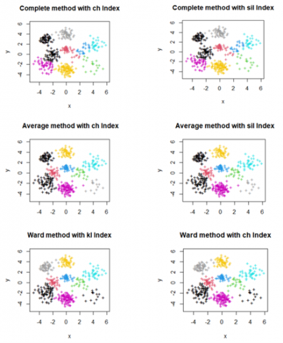
The results of the simulation are presented in Tables 5 to 12 and Figures 2 to 5. Figure 2 shows the true clusters for the models (Model 1, _ve groups), (Model 2, nine groups), (Model 3, eight groups), (Model 4, ten groups). Tables 5, 7, 9, 11 show the number of clusters for the simulated models by using some clustering methods with some indices, while Tables 6, 8, 10, 12 illustrate the rate of agreement between the true clusters and the results of the clustering methods with internal similarity indices using some external indices (Rand, F-M, Purity). In these results we can see the following:
Figure 2. (a) True clusters for (Model 1, number of clusters is 5); (b) True clusters for (Model 2, number of clusters is 9); (c) True clusters for (Model 3, number of clusters is 8); (d) True clusters for (Model 4, number of clusters is 10)
Figure 3. Clustering methods (average, ward.D2, median) with some internal indices (KL, CH)
Figure 4. Clustering methods (complete, average, Ward.D2) with some internal indices (KL, CH, Sil)
Table 5. Number of clusters for data points (Model 1) using clustering methods with internal indices and two types of distance measures (Euclidean and Manhattan)
|
|
Euclidean Distance |
Manhattan Distance |
||||||
|
|
KL |
CH |
Sil |
Gap |
KL |
CH |
Sil |
Gap |
|
Single |
8 |
8 |
2 |
2 |
6 |
6 |
2 |
2 |
|
Complete |
4 |
4 |
2 |
2 |
4 |
4 |
2 |
2 |
|
Average |
4 |
5 |
2 |
2 |
4 |
5 |
4 |
2 |
|
Centroid |
2 |
4 |
2 |
2 |
8 |
4 |
2 |
2 |
|
Ward.D2 |
4 |
5 |
2 |
4 |
4 |
5 |
2 |
4 |
|
Median |
5 |
5 |
3 |
5 |
7 |
7 |
4 |
7 |
Table 6. The rate of agreement between the true clusters and the partitions that we have computed for (Model 1) using external similarity indices under Euclidean distance and Manhattan distance
|
|
Euclidean Distance |
Manhattan Distance |
||||
|
Clustering methods |
Rand |
F-M |
Purity |
Rand |
F-M |
Purity |
|
Single, KL |
0.759 |
0.646 |
0.608 |
0.529 |
0.527 |
0.416 |
|
Single, CH |
0.759 |
0.646 |
0.608 |
0.529 |
0.527 |
0.416 |
|
Single, Sil |
0.201 |
0.441 |
0.204 |
0.201 |
0.441 |
0.204 |
|
Single, Gap |
0.201 |
0.441 |
0.204 |
0201 |
0.441 |
0.204 |
|
Complete, KL |
0.899 |
0.791 |
0.776 |
0.886 |
0.767 |
0.760 |
|
Complete, CH |
0.899 |
0.791 |
0.776 |
0.886 |
0.767 |
0.760 |
|
Complete, Sil |
0.672 |
0.601 |
0.400 |
0.672 |
0.601 |
0.400 |
|
Complete, Gap |
0.672 |
0.601 |
0.400 |
0.672 |
0.601 |
0.400 |
|
Average, KL |
0.907 |
0.813 |
0.792 |
0.894 |
0.775 |
0.792 |
|
Average, CH |
0.944 |
0.859 |
0.920 |
0.918 |
0.809 |
0.856 |
|
Average, Sil |
0.672 |
0.601 |
0.400 |
0.894 |
0.775 |
0.792 |
|
Average, Gap |
0.672 |
0.601 |
0.400 |
0.511 |
0.529 |
0.396 |
|
Centroid, KL |
0.672 |
0.601 |
0.400 |
0.917 |
0.800 |
0.864 |
|
Centroid, CH |
0.906 |
0.808 |
0.788 |
0.899 |
0.803 |
0.780 |
|
Centroid, Sil |
0.672 |
0.601 |
0.400 |
0.664 |
0.599 |
0.400 |
|
Centroid, Gap |
0.672 |
0.601 |
0.400 |
0.664 |
0.599 |
0.400 |
|
Ward.D2, KL |
0.910 |
0.819 |
0.796 |
0.910 |
0.819 |
0.796 |
|
Ward.D2, CH |
0.949 |
0.872 |
0.928 |
0.947 |
0.867 |
0.924 |
|
Ward.D2, Sil |
0.672 |
0.601 |
0.400 |
0.672 |
0.601 |
0.400 |
|
Ward.D2, Gap |
0.910 |
0.819 |
0.796 |
0.910 |
0.819 |
0.796 |
|
Median, KL |
0.908 |
0.818 |
0.792 |
0.865 |
0.690 |
0.772 |
|
Median, CH |
0.908 |
0.818 |
0.792 |
0.865 |
0.690 |
0.772 |
|
Median, Sil |
0.759 |
0.661 |
0.600 |
0.755 |
0.642 |
0.596 |
|
Median, Gap |
0.908 |
0.818 |
0.792 |
0.865 |
0.690 |
0.772 |
Figure 5. Clustering methods (average, ward.D2, median) with some internal indices (CH, Sil) .These methods show an equality between the number of clusters and the number of true clusters
Table 7. Number of clusters for data points (Model 2) using clustering methods with internal indices and two types of distance measures (Euclidean and Manhattan)
|
|
Euclidean Distance |
Manhattan Distance |
||||||
|
|
KL |
CH |
Sil |
Gap |
KL |
CH |
Sil |
Gap |
|
Single |
12 |
12 |
12 |
2 |
4 |
7 |
7 |
2 |
|
Complete |
12 |
9 |
9 |
3 |
9 |
8 |
8 |
2 |
|
Average |
10 |
9 |
9 |
2 |
10 |
9 |
9 |
2 |
|
Centroid |
7 |
10 |
7 |
2 |
7 |
8 |
7 |
2 |
|
Ward.D2 |
9 |
9 |
9 |
2 |
9 |
9 |
9 |
2 |
|
Median |
12 |
12 |
12 |
12 |
6 |
7 |
8 |
6 |
Table 8. The rate of agreement between the true clusters and the partitions that we have computed for (Model 2) using external similarity indices under Euclidean distance and Manhattan distance
|
|
Euclidean Distance |
Manhattan Distance |
||||
|
Clustering methods |
Rand |
F-M |
Purity |
Rand |
F-M |
Purity |
|
Single, KL |
0.710 |
0.556 |
0.604 |
0.198 |
0.377 |
0.258 |
|
Single, CH |
0.710 |
0.556 |
0.604 |
0.598 |
0.498 |
0.516 |
|
Single, Sil |
0.710 |
0.556 |
0.604 |
0.598 |
0.498 |
0.516 |
|
Single, Gap |
0.138 |
0.367 |
0.226 |
0138 |
0.367 |
0.226 |
|
Complete, KL |
0.958 |
0.837 |
0.914 |
0.973 |
0.906 |
0.910 |
|
Complete, CH |
0.972 |
0.896 |
0.914 |
0.974 |
0.907 |
0.910 |
|
Complete, Sil |
0.972 |
0.896 |
0.914 |
0.974 |
0.907 |
0.910 |
|
Complete, Gap |
0.767 |
0.602 |
0.447 |
0.363 |
0.415 |
0.314 |
|
Average, KL |
0.981 |
0.932 |
0.959 |
0.979 |
0.922 |
0.955 |
|
Average, CH |
0.982 |
0.936 |
0.959 |
0.981 |
0.932 |
0.955 |
|
Average, Sil |
0.982 |
0.936 |
0.959 |
0.981 |
0.932 |
0.955 |
|
Average, Gap |
0.413 |
0.429 |
0.314 |
0.416 |
0.430 |
0.314 |
|
Centroid, KL |
0.952 |
0.856 |
0.822 |
0.951 |
0.850 |
0.817 |
|
Centroid, CH |
0.986 |
0.950 |
0.968 |
0.957 |
0.865 |
0.862 |
|
Centroid, Sil |
0.952 |
0.856 |
0.822 |
0.951 |
0.850 |
0.817 |
|
Centroid, Gap |
0.350 |
0.413 |
0.314 |
0.195 |
0.378 |
0.256 |
|
Ward.D2, KL |
0.980 |
0.928 |
0.955 |
0.982 |
0.935 |
0.957 |
|
Ward.D2, CH |
0.980 |
0.928 |
0.955 |
0.982 |
0.935 |
0.957 |
|
Ward.D2, Sil |
0.980 |
0.928 |
0.955 |
0.982 |
0.935 |
0.957 |
|
Ward.D2, Gap |
0.632 |
0.515 |
0.357 |
0.632 |
0.515 |
0.357 |
|
Median, KL |
0.959 |
0.850 |
0.928 |
0.875 |
0.680 |
0.635 |
|
Median, CH |
0.959 |
0.850 |
0.928 |
0.901 |
0.722 |
0.714 |
|
Median, Sil |
0.959 |
0.850 |
0.928 |
0.904 |
0.726 |
0.746 |
|
Median, Gap |
0.959 |
0.850 |
0.928 |
0.875 |
0.680 |
0.635 |
Table 9. Number of clusters for data points (Model 3) using clustering methods with internal indices and two types of distance measures (Euclidean and Manhattan)
|
|
Euclidean Distance |
Manhattan Distance |
||||||
|
|
KL |
CH |
Sil |
Gap |
KL |
CH |
Sil |
Gap |
|
Single |
9 |
9 |
2 |
2 |
5 |
6 |
2 |
2 |
|
Complete |
4 |
8 |
8 |
2 |
10 |
8 |
8 |
2 |
|
Average |
4 |
8 |
8 |
2 |
12 |
8 |
8 |
2 |
|
Centroid |
5 |
9 |
9 |
2 |
4 |
10 |
10 |
2 |
|
Ward.D2 |
8 |
10 |
8 |
2 |
8 |
8 |
8 |
2 |
|
Median |
2 |
7 |
7 |
2 |
3 |
10 |
10 |
2 |
Table 10. The rate of agreement between the true clusters and the partitions that we have computed for (Model 3) using external similarity indices under Euclidean distance and Manhattan distance
|
|
Euclidean Distance |
Manhattan Distance |
||||
|
Clustering methods |
Rand |
F-M |
Purity |
Rand |
F-M |
Purity |
|
Single, KL |
0.150 |
0.350 |
0.158 |
0.136 |
0.352 |
0.150 |
|
Single, CH |
0.339 |
0.390 |
0.266 |
0.327 |
0.392 |
0.257 |
|
Single, Sil |
0.128 |
0.354 |
0.144 |
0.128 |
0.354 |
0.144 |
|
Single, Gap |
0.128 |
0.354 |
0.144 |
0128 |
0.354 |
0.144 |
|
Complete, KL |
0.810 |
0.584 |
0.514 |
0.961 |
0.839 |
0.935 |
|
Complete, CH |
0.942 |
0.784 |
0.880 |
0.967 |
0.873 |
0.935 |
|
Complete, Sil |
0.942 |
0.784 |
0.880 |
0.967 |
0.873 |
0.935 |
|
Complete, Gap |
0.583 |
0.452 |
0.286 |
0.613 |
0.475 |
0.285 |
|
Average, KL |
0.821 |
0.621 |
0.530 |
0.966 |
0.866 |
0.941 |
|
Average, CH |
0.968 |
0.876 |
0.937 |
0.968 |
0.875 |
0.937 |
|
Average, Sil |
0.968 |
0.876 |
0.937 |
0.968 |
0.875 |
0.937 |
|
Average, Gap |
0.582 |
0.476 |
0.285 |
0.582 |
0.469 |
0.285 |
|
Centroid, KL |
0.736 |
0.546 |
0.483 |
0.739 |
0.552 |
0.485 |
|
Centroid, CH |
0.960 |
0.844 |
0.921 |
0.936 |
0.854 |
0.926 |
|
Centroid, Sil |
0.960 |
0.844 |
0.921 |
0.963 |
0.854 |
0.926 |
|
Centroid, Gap |
0.128 |
0.354 |
0.144 |
0.305 |
0.386 |
0.242 |
|
Ward.D2, KL |
0.940 |
0.776 |
0.878 |
0.959 |
0.844 |
0.919 |
|
Ward.D2, CH |
0.945 |
0.768 |
0.885 |
0.959 |
0.844 |
0.919 |
|
Ward.D2, Sil |
0.940 |
0.776 |
0.878 |
0.959 |
0.844 |
0.919 |
|
Ward.D2, Gap |
0.527 |
0.428 |
0.285 |
0.607 |
0.467 |
0.285 |
|
Median, KL |
0.317 |
0.394 |
0.250 |
0.248 |
0.355 |
0.214 |
|
Median, CH |
0.860 |
0.610 |
0.648 |
0.835 |
0.551 |
0.676 |
|
Median, Sil |
0.860 |
0.610 |
0.648 |
0.853 |
0.551 |
0.676 |
|
Median, Gap |
0.317 |
0.394 |
0.250 |
0.248 |
0.355 |
0.214 |
Table 11. Number of clusters for data points (Model 4) using clustering methods with internal indices and two types of distance measures (Euclidean and Manhattan)
|
|
Euclidean Distance |
Manhattan Distance |
||||||
|
|
KL |
CH |
Sil |
Gap |
KL |
CH |
Sil |
Gap |
|
Single |
6 |
8 |
8 |
2 |
3 |
2 |
2 |
4 |
|
Complete |
4 |
10 |
8 |
2 |
4 |
10 |
8 |
2 |
|
Average |
4 |
10 |
10 |
2 |
4 |
10 |
11 |
2 |
|
Centroid |
4 |
12 |
8 |
2 |
4 |
8 |
8 |
3 |
|
Ward.D2 |
10 |
10 |
10 |
2 |
10 |
10 |
10 |
2 |
|
Median |
4 |
11 |
6 |
4 |
9 |
7 |
7 |
9 |
Table 12. The rate of agreement between the true clusters and the partitions that we have computed for (Model 4) using external similarity indices under Euclidean distance and Manhattan distance
|
|
Euclidean Distance |
Manhattan Distance |
||||
|
Clustering Methods |
Rand |
F-M |
Purity |
Rand |
F-M |
Purity |
|
Single, KL |
0.673 |
0.482 |
0.400 |
0.674 |
0.471 |
0.347 |
|
Single, CH |
0.860 |
0.644 |
0.631 |
0.508 |
0.412 |
0.231 |
|
Single, Sil |
0.860 |
0.644 |
0.631 |
0.508 |
0.412 |
0.231 |
|
Single, Gap |
0.255 |
0.344 |
0.200 |
0.681 |
0.489 |
0.431 |
|
Complete, KL |
0.795 |
0.573 |
0.431 |
0.795 |
0.573 |
0.431 |
|
Complete, CH |
0.974 |
0.874 |
0.917 |
0.965 |
0.834 |
0.894 |
|
Complete, Sil |
0.949 |
0.803 |
0.829 |
0.939 |
0.775 |
0.814 |
|
Complete, Gap |
0.581 |
0.440 |
0.231 |
0.601 |
0.448 |
0.231 |
|
Average, KL |
0.795 |
0.573 |
0.431 |
0.795 |
0.573 |
0.431 |
|
Average, CH |
0.989 |
0.948 |
0.972 |
0.989 |
0.946 |
0.972 |
|
Average, Sil |
0.989 |
0.948 |
0.972 |
0.989 |
0.946 |
0.972 |
|
Average, Gap |
0.581 |
0.440 |
0.231 |
0.581 |
0.440 |
0.231 |
|
Centroid, KL |
0.795 |
0.573 |
0.431 |
0.795 |
0.573 |
0.431 |
|
Centroid, CH |
0.989 |
0.944 |
0.972 |
0.949 |
0.802 |
0.814 |
|
Centroid, Sil |
0.941 |
0.790 |
0.823 |
0.949 |
0.802 |
0.814 |
|
Centroid, Gap |
0.255 |
0.344 |
0.200 |
0.634 |
0.464 |
0.315 |
|
Ward.D2, KL |
0.989 |
0.948 |
0.972 |
0.988 |
0.941 |
0.968 |
|
Ward.D2, CH |
0.989 |
0.948 |
0.972 |
0.988 |
0.941 |
0.968 |
|
Ward.D2, Sil |
0.989 |
0.948 |
0.972 |
0.988 |
0.941 |
0.968 |
|
Ward.D2, Gap |
0.581 |
0.440 |
0.231 |
0.581 |
0.440 |
0.231 |
|
Median, KL |
0.746 |
0.507 |
0.400 |
0.912 |
0.683 |
0.711 |
|
Median, CH |
0.955 |
0.798 |
0.848 |
0.913 |
0.696 |
0.711 |
|
Median, Sil |
0.812 |
0.565 |
0.600 |
0.913 |
0.696 |
0.711 |
|
Median, Gap |
0.746 |
0.507 |
0.400 |
0.912 |
0.683 |
0.711 |
5.1 Conclusion
Different models and different distance measures have been used in this paper to evaluate the performance of some clustering methods (single linkage, complete linkage, average inkage, centroid, ward.2D, median) under different validity indices (KL, CH, Sil, Gap), different simulated data with different sample sizes using R software 3.1. Also, some external indices (Rand, F-M, Purity) are used to get the rate of agreement between the true clusters of the data points and the partitions that we have computed using clustering methods. For the results we noticed the following:
5.2 Future works
In this study, we only evaluate the performance of some clustering methods with some indices under linear data only, but it will be also interesting to explore how these clustering methods and indices works under circular data. Also, in the future we look forward to construct a novel clustering method and evaluate the performance of the proposed clustering method with the average linkage method with CH index.
[1] Rocha, L.M., Cappabianco, F.A., Falcão, A.X. (2009). Data clustering as an optimum-path forest problem with applications in image analysis. International Journal of Imaging Systems and Technology, 19(2): 50-68.
[2] Kassambara, A. (2017). Practical Guide to Cluster Analysis in R: Unsupervised Machine Learning. Sthda.
[3] Abushilah, S.F.H. (2019). Clustering methodology for bivariate circular data with application to protein dihedral angles. Doctoral dissertation, University of Leeds.
[4] Diday, E., Govaert, G., Lechevallier, Y., Sidi, J. (1981). Clustering in pattern recognition. In: Simon, J.C., Haralick, R.M. (eds) Digital Image Processing. NATO Advanced Study Institutes Series, vol 77. Springer, Dordrecht. https://doi.org/10.1007/978-94-009-8543-8_2
[5] Mirkin, B. (2005). Clustering for Data Mining: A Data Recovery Approach. Chapman and Hall/CRC.
[6] Landau, S., Leese, M., Stahl, D., Everitt, B.S. (2011). Cluster Analysis. John Wiley & Sons.
[7] Mardia, K.V., Kent, J.T., Bibby, J. (1979). Multivariate Analysis. Academic Press; London.
[8] Manly, B.F., Alberto, J.A.N. (2016). Multivariate Statistical Methods: A Primer. Chapman and Hall/CRC.
[9] Frades, I., Matthiesen, R. (2010). Overview on techniques in cluster analysis. In: Matthiesen, R. (eds) Bioinformatics Methods in Clinical Research. Methods in Molecular Biology, vol 593. Humana Press. https://doi.org/10.1007/978-1-60327-194-3_5
[10] Murtagh, F., Contreras, P. (2011). Methods of hierarchical clustering. arXiv preprint arXiv:1105.0121. https://doi.org/10.48550/arXiv.1105.0121
[11] Gupta, G.K. (2014). Introduction to Data Mining with case Studies. PHI Learning Pvt. Ltd.
[12] Caliński, T., Harabasz, J. (1974). A dendrite method for cluster analysis. Communications in Statistics-theory and Methods, 3(1): 1-27.
[13] Rousseeuw, P.J. (1987). Silhouettes: A graphical aid to the interpretation and validation of cluster analysis. Journal of Computational and Applied Mathematics, 20: 53-65. https://doi.org/10.1016/0377-0427(87)90125-7
[14] Krzanowski, W.J., Lai, Y.T. (1988). A criterion for determining the number of groups in a data set using sum-of-squares clustering. Biometrics, 44(1): 23-34. https://doi.org/10.2307/2531893
[15] Tibshirani, R., Walther, G., Hastie, T. (2001). Estimating the number of clusters in a data set via the gap statistic. Journal of the Royal Statistical Society: Series B (Statistical Methodology), 63(2): 411-423. https://doi.org/10.1111/1467-9868.00293
[16] Charrad, M., Ghazzali, N., Boiteau, V., Niknafs, A. (2014). NbClust: An R package for determining the relevant number of clusters in a data set. Journal of Statistical Software, 61: 1-36. https://doi.org/10.18637/jss.v061.i06
[17] Rand, W.M. (1971). Objective criteria for the evaluation of clustering methods. Journal of the American Statistical Association, 66(336): 846-850.
[18] Rendón, E., Abundez, I., Arizmendi, A., Quiroz, E.M. (2011). Internal versus external cluster validation indexes. International Journal of Computers and Communications, 5(1): 27-34.
[19] Chalise, P., Raghavan, R., Fridley, B. (2016). IntNMF: Integrative clustering of multiple genomic dataset.
[20] Fowlkes, E.B., Mallows, C.L. (1983). A method for comparing two hierarchical clusterings. Journal of the American Statistical Association, 78(383): 553-569.