Reyam G. Ghane*![]() | Mohammed Y. Hassan
| Mohammed Y. Hassan![]()
© 2023 IIETA. This article is published by IIETA and is licensed under the CC BY 4.0 license (http://creativecommons.org/licenses/by/4.0/).
OPEN ACCESS
This paper presents a novel nonlinear control strategy tailored for foldable quadrotors capable of altering their morphology in-flight. By changing the quadrotor's shape through servo motors, these adaptive systems can effectively overcome various challenges, including diverse environmental conditions, such as obstacles and climate variations. The proposed control approach utilizes a double-loop control method to enhance the robustness and performance of the folding quadrotor during flight. The outer loop consists of a nonlinear PID controller responsible for regulating motion in the X and Y directions, while the inner loop features a sliding mode controller for altitude control in the Z direction and attitude stabilization. This dual-loop structure ensures the quadrotor's stability even during arm folding. The firefly algorithm is employed to optimize the parameters of both controllers, minimizing position errors using the Root Mean Square Error (RMSE) as a performance metric. Our results demonstrate a significant improvement in the quadrotor's performance and adaptability to various proposed morphologies, with error rates reduced to near-negligible levels for all shapes. Specifically, the X position error was reduced by 100% for all morphologies, the Y position error by 95% for the X shape, 97% for the T shape, 98% for the H shape, and 99% for the O shape, and the Z position error by 99% for all morphologies.
nonlinear PID control, sliding mode control, foldable quadrotor
In recent years, quadrotors have garnered significant attention from researchers and scientists due to their potential applications in various fields, both civilian and military. These applications include search and rescue, surveillance, photography, and delivery [1]. Consequently, numerous studies have been conducted to enhance the stability of quadrotors during flight [2, 3] and to improve their utility in delivery applications [4, 5]. However, conventional quadrotor designs are not well-suited for navigating small spaces and irregular surfaces, owing to their inherent stability. This limitation has led to a growing demand for adaptable quadrotors capable of maintaining in-flight stability while encountering obstacles.
To address this need, several researchers have proposed variable-geometry quadrotors capable of altering their shape using techniques such as origami or by simulating bird flight [6-9]. Nonetheless, morphological changes can compromise quadrotor stability, necessitating the development of specialized control systems. For instance, Model Reference Adaptive Control was implemented to control the angular velocity of an X-morphology quadrotor and account for shifts in the center of gravity, proving effective in adapting to folding maneuvers [10]. However, the alignment of the servo motor's axis with the robot's center of rotation weakens the mechanical structure [10]. A PID controller was designed for a quad-morphing robot, but roll control was lost when the robot was folded due to the alignment of the four rotors [11]. The feedback control module, designed using a Lyapunov stabilization approach, effectively tracked the desired roll angle but became less efficient when the arms were folded, increasing the risk of collision [12]. The Linear Quadratic Regulator controller, in conjunction with the computation of the inertia matrix, ensured stable flight but reduced the aircraft's flight time [13]. The backstepping controller, with parameters optimized using the PSO algorithm, showed acceptable stability, precision, and speed in simulations, but required manual changing of configurations, limiting the quadrotor's autonomy [14].
In this study, the problem of maintaining stability during morphological changes and tracking the desired trajectory of a foldable quadrotor is addressed. A double-loop control strategy is developed, utilizing two types of nonlinear controllers, namely Sliding Mode Control (SMC) and Nonlinear PID. The primary objective is to design the proposed inner and outer loop controllers, optimizing their parameters using the firefly algorithm to minimize position errors across various quadrotor shapes while ensuring flight continuity during shape changes.
The remainder of this paper is organized as follows: The mechanical design of the foldable quadrotor and the effects of its center of gravity are described in Section 2. The proposed controllers for the foldable quadrotor are elucidated in Section 3. The proposed control unit design is presented in detail in Section 4. An overview of the firefly algorithm and its application for parameter optimization are provided in Section 5. The simulation results are discussed in detail in Section 6. Finally, conclusions are offered in Section 7.
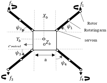
The foldable quadrotor, as shown in Figure 1, consists of a rigid central body $m_o$ and four arms of masses m2,i that is foldable around the main body using servo motors and at different angles, see Table 1 [15]. Since these angles represent the extension of the folded arm by calculating the potential control matrix for each shape, the possible shapes of this quad are (X, H, O, Y, YI, T) [14]. Servo motors of masses $m_{1, i}$ are connected to the central body and the four arms are connected to the servo motors, as well as four rotors of masses $m_{3, i}$ are located on the arms. Two rotors (2 and 4) are rotated in a clockwise direction and other two rotors (1 and 3) are rotated in a counterclockwise direction. Due to changing the quadrotor's morphology, the servo motors make the system highly coupled. The main body and servo motors are fixed around Z-axis while the arms and rotors rotate on the same axis (Z-axis). So, the most (conventional) setup leads to numerous conceivable arrangements by changing the position of the arms [15].
Some assumptions are presented to make a suitable model for the foldable quadrotor [16]:
Figure 1. Schematic of the foldable quadrotor [15]
Table 1. Characteristics of the foldable quadrotor configuration [14]
|
Configuration |
Arm Angles |
|||
|
ψ1(t) |
ψ2(t) |
ψ3(t) |
ψ4(t) |
|
|
X |
π⁄4 |
π⁄4 |
π⁄4 |
π⁄4 |
|
H |
π⁄2 |
0 |
π⁄2 |
0 |
|
O |
π |
π |
π |
π |
|
Y |
π⁄4 |
π⁄4 |
π⁄2 |
0 |
|
YI |
π⁄2 |
0 |
π⁄4 |
π⁄4 |
|
T |
0 |
π⁄2 |
π⁄2 |
0 |
2.1 Kinematic model of a foldable quadrotor
The mathematical model of the quadrotor is described in two frames see Figure 1. The body frame Rb(Ob, Xb, Yb, Zb), which is fixed and the mobile frame Rm(Om, Xm, Ym, Zm). The rotation from Rb to Rm consists of three revolutions around an (X, Y, Z) axes, which means that the position is obtained at an angle (φ, ψ). So, the total rotation matrix R can be given as [15]:
$R=\left[\begin{array}{ccc}c \psi c \theta & c \psi s \theta s \varphi-s \psi c \varphi & c \psi s \theta c \varphi+s \psi s \varphi \\ s \psi c \theta & s \psi s \theta s \varphi+c \psi c \varphi & s \psi s \theta c \varphi-c \psi s \varphi \\ -s \theta & c \theta s \varphi & c \theta c \varphi\end{array}\right]$ (1)
where, $R \in S O(3)=\left\{R \in R^{3 \times 3} \mid R^T R=I_{3 \times 3, \operatorname{det}(R)=1\quad}\right\} \mathrm{s}($.$)\quad and\quad c(.)$ are abbreviations for sin(.) and cos(.), respectively. The linear velocity of the system is represented by $\mathrm{A}=\left[\begin{array}{lll}u & v & w\end{array}\right]^T \in R^3$ and angular velocity is represented by $\varsigma=\left[\begin{array}{lll}p & q & r\end{array}\right]^T \in R^3$. Both of the velocities are derived in the mobile frame Rm. The mass of the foldable quadrotor is m and the inertia is represented as $\left(\psi_i(t)\right) \in R^{3 \times 3}$. $\xi=\left[\begin{array}{lll}X & Y & Z\end{array}\right]^T \in R^3$ describes the position and $\eta=\left[\begin{array}{lll}\varphi & \theta & \psi\end{array}\right]^T \in R^3$ describes the orientation of the quadrotor.
2.2 Dynamic model of a foldable quadrotor
The dynamic model of the foldable quadrotor is derived from the Newton-Euler formalism and given as follows [14]:
$\left[\begin{array}{cc}m J_{3 \times 3}\left(\psi_i(t)\right) & O_{3 \times 3} \\ O_{3 \times 3} & J_{3 \times 3}\left(\psi_i(t)\right)\end{array}\right]\left[\begin{array}{c}\dot{\mathrm{A}} \\ \dot{\zeta}\end{array}\right]+\left[\begin{array}{c}\varsigma \times m \mathrm{~A} \\ \varsigma \times J\left(\psi_i(t)\right)\end{array}\right]=\left[\begin{array}{c}f \\ \tau\end{array}\right]$ (2)
where, O3×3 is a zero-matrix dimensional 3×3, and × denotes the cross product.
Many forces act on the quadrotor, such as gravity, thrust, hub and drag. So, the total force in the mobile frame is expressed [14]:
$f=\left[\begin{array}{l}U_x \\ U_y \\ F_t\end{array}\right]+R^T\left[\begin{array}{l}F_{D x} \\ F_{D y} \\ F_{D z}\end{array}\right]+R^T\left[\begin{array}{c}0 \\ 0 \\ -m g\end{array}\right]$ (3)
The relation between the velocities and the external forces is $f=\left[f_x f_y f_z\right]^T \in R^3$ and $f_g=[00-m g]^T$ is the gravity vector, where $g$ is the gravity. $F_t$ Is The total thrust force generated by the rotation of each rotor, two components represent the hub forces $U_x, U_y$. Also, the quadrotor generates drag force $F_D \in R^3$ in the body.
The quadrotor can turn around $x_m, y_m, z_m$ directions by applying the moments $\tau_{\varphi}, \tau_\theta, \tau_\psi$. These moments depend on the folding angles of the arms and are induced by thrust forces $F_t$. Thus, the moments of roll, pitch and yaw are in the study [14].
$\tau=\left[\begin{array}{c}\tau_{\varphi}+O_x+L_x+M_{A X} \\ \tau_\theta+O_y+L_y+M_{A Y} \\ \tau_\psi+H+M_{A Z}\end{array}\right]$ (4)
Wind effects can produce an aerodynamic friction torque as [14].
$M_A=\left[M_{A x} M_{A y} M_{A z}\right]^T=\operatorname{diag}\left(k_{a x} k_{a y} k_{a z}\right) \dot{\zeta}^2$ (5)
where, $k_{a(x, y, z)}$ is the aerodynamic friction coefficient.
(Ox, Oy) Are the Gyroscopic moments, (Lx, Ly) are the flapping moment, and (H) is the hub moment. However, some phenomena have a slight effect, such as hub forces and blade flapping moments. Thus, they are neglected because the quadrotor adopted in this research does not perform any aggressive rotation of the four arms during flight [15].
2.3 Center of gravity
The possible shapes of the folding quadrotor are asymmetrical, so the center of gravity changes from one form to another, as each state has its center of gravity. As a result, it is necessary to calculate the center of gravity for each shape. The general formula of the center of gravity is shown below [6]:
$O G=\frac{\sum_{i=1}^4 \sum_{j=1}^3 \quad m_{j, i} \quad\overline{O G_{J, l}}}{m_o+\sum_{i=1}^4 \sum_{j=1}^3 \quad m_{j, i}}$ (6)
where:
$\mathrm{O}$ is the geometric center.
$\overrightarrow{O G}$ is the offset between the geometric center of the system and the global center of gravity.
$\overrightarrow{O G_o} \in R^{3 \times 1}$ is the vector of the center of gravity of the central body, which is zero.
$\overrightarrow{O G_{1, l}} \in R^{3 \times 1}$ is the vector of the center of gravity of the servo motors.
$\overrightarrow{O G_{2, l}} \in R^{3 \times 1}$ is the vector of the center of gravity of the rotating arms.
$\overrightarrow{O G_{3, l}} \in R^{3 \times 1}$ is the vector of the center of gravity of the rotors.
2.4 Control matrix
The control matrix presents the critical values of the foldable quadrotor control architecture, as it converts the square of the rotational speed of the four propellers $\left(\left.\Omega_i^2\right|_{i=1,2,3,4}\right)$ into the total thrust force $F_t$ and moments $\tau_{\varphi}, \tau_\theta, \tau_\psi\quad$ [6]:
$\Delta\left(\psi_i(t)\right)=\left[\begin{array}{cccc}b & b\left(y_{3,1}-y_g\right) & b\left(x_g-x_{3,1}\right) & d \\ b & b\left(y_{3,2}-y_g\right) & b\left(x_g-x_{3,2}\right) & -d \\ b & b\left(y_{3,3}-y_g\right) & b\left(x_g-x_{3,3}\right) & d \\ b & b\left(y_{3,4}-y_g\right) & b\left(x_g-x_{3,4}\right) & -d\end{array}\right]^T$ (7)
Define the control vector of its altitude and attitude as [6]: $u=\left[\begin{array}{llll}u_1 & u_2 & u_3 & u_4\end{array}\right]^T \in R^{4 \times 4}$, where,
$\left[\begin{array}{l}u_1 \\ u_2 \\ u_3 \\ u_4\end{array}\right]=\Delta\left(\psi_i(t)\right)\left[\begin{array}{l}\Omega_1^2 \\ \Omega_2^2 \\ \Omega_3^2 \\ \Omega_4^2\end{array}\right]$ (8)
b and d are the aerodynamic coefficients and are taken as [6]:
$f_i=b \Omega_i^2, Q_i=d \Omega_i^2$ (9)
where, b is the Thrust coefficient and d is the drag coefficient.
The foldable quadrotor has eight control inputs. The primary four inputs deliver the control vector altitude and attitude. The second four control inputs provide the servo motors' control vector. To establish the complete dynamic model, a state space vector is given, which consists of a set of inputs, outputs and states associated with first-order differential equations, which will form a model of the space. A space with state variables as its axes is referred to as a "state space”. The state of the system can be represented as a vector. The general state space model is represented as following:
$\left\{\begin{array}{c}\dot{x}(t)=A x(t)+B u(t) \\ y(t)=c x(t)\end{array}\right.$ (10)
where, x(t), y(t), and u(t) presented the state, output and control vector, respectively. A, B, and C shows system matrix, input and output matrix, respectively.
So, based on Eqs. (2), (3) and (4), the state space vector of the nonlinear dynamic model is given as [14]:
$\mathrm{X}=\lceil\mathrm{x} \dot{\mathrm{x}} \mathrm{y} \dot{\mathrm{y}} \mathrm{z} \dot{\mathrm{z}} \varphi \dot{\varphi} \theta \dot{\theta} \psi \dot{\psi}\rceil^T$ (11)
Also, the state space vector is written as [14]:
$X=\left[\begin{array}{lllllllllllll}x_1 & x_2 & x_3 & x_4 & x_5 & x_6 & x_7 & x_8 & x_9 & x_{10} & x_{11} & x_{12}\end{array}\right]^T$ (12)
$\left\{\begin{array}{c}\dot{x}_1=x_2 \\ \dot{x}_2=U_1 \frac{u_x}{m}+b_1 x_2 \\ \dot{x}_3=x_4 \\ \dot{x}_4=U_1 \frac{u_y}{m}+b_2 x_4 \\ \dot{x}_5=x_6 \\ \dot{x}_6=-g+U_1 \frac{\cos \varphi \cos \theta}{m}+b_3 x_6 \\ \dot{x}_7=x_8 \\ \dot{x}_8=a_1 \dot{\theta} \dot{\psi}+a_4 \dot{\theta} \Omega_r+\frac{1}{J_{x x}} U_2+b_4 \dot{\varphi}^2 \\ \dot{x}_9=x_{10} \\ \dot{x}_{10}=a_2 \dot{\varphi} \dot{\psi}+a_5 \dot{\varphi} \Omega_r+\frac{1}{J_{y y}} U_3+b_5 \dot{\theta}^2 \\ \dot{x}_{11}=x_{12} \\ \dot{x}_{12}=a_3 \dot{\varphi} \dot{\theta}+\frac{1}{J_{z z}} U_4+b_6 \dot{\psi}^2\end{array}\right.$ (13)
where, $a_1=\frac{J_{y y}-J_{z z}}{J_{x x}}, a_2=\frac{J_{z z}-J_{x x}}{J_{y y}}, a_3=\frac{J_{x x}-J_{y y}}{J_{z z}}, a_4=\frac{-J_r}{J_{x x}}$, $a_5=\frac{J_r}{J_{y y}}, \quad b_1=\frac{-k_{D x}}{m}, b_2=\frac{-k_{D y}}{m}, b_3=\frac{-k_{D z}}{m}, b_4=\frac{-k_{A x}}{J_{x x}}$, $b_5=\frac{-k_{A y}}{J_{y y}}, b_6=\frac{-k_{A z}}{J_{z z}}$
$u_x=\sin \Psi \sin \varphi+\cos \Psi \sin \theta \cos \varphi$ (14)
$u_y=\sin \Psi \sin \theta \cos \varphi-\cos \Psi \sin \varphi$ (15)
$\Omega_r=\Omega_1^2-\Omega_2^2+\Omega_3^2-\Omega_4^2$ (16)
The foldable quadrotor is a nonlinear, underactuated system, as well as a strong coupling due to servo motors that connect each arm to the main body making the system highly coupled. It has only four control inputs but must control six states as an underactuated system. As a result of these reasons, the double loop control strategy relied upon using two types of controllers, where the control system is divided into two parts. The first part is where the input control is available, called the inner loop control, and uses the classic sliding mode control. While the second part is where no actual control input is available, it is called outer loop control and uses nonlinear PID.
3.1 Classical sliding mode controller
The sliding mode control is one of the methods used to control nonlinear systems, as it provides an efficient design to ensure the stability of the control unit [17]. The sliding mode control consists of two main parts:
$u=u_{e q}+u_{d i s}$ (17)
where, ueq is the nominal control part, udis. It is the discontinuous part. Define the discontinuous part as [18]:
$u_{\text {dis }}=-k \operatorname{sign}(s)$ (18)
where, s is the sliding surface and it is assumed as:
$s=\dot{e}+c e$ (19)
3.2 Nonlinear PID controller
The traditional PID has been developed to have a greater degree of freedom to be more scalable to design for nonlinear systems It was reconstructed by replacing the linear PID parts with nonlinear functions as shown in the equations below [19]:
$U_{N L P I D}=f_1(e)+f_2(\dot{e})+f_3\left(\int e d t\right)$ (20)
$f_i=k_i(\beta)|\beta|^{\alpha_i} \operatorname{sign}(\beta)$ (21)
$k_i(\beta)=k_{i 1}+\frac{k_{i 2}}{1+\exp \left(\mu_i \beta^2\right)}, i=1,2,3$ (22)
The design process for the inner loop (u1, u2, u3 u4) is based on the sliding mode control method, while the design for control signals (ux, uy) for the motion in the (x, y) plane are based on the nonlinear PID (NLPID) control, see Figure 2.
Figure 2. Proposed foldable quadrotor control design
4.1 Design of inner loop Sliding Mode Controller (SMC)
For the altitude (Z) [14]:
$\left\{\begin{array}{c}\dot{x}_5=x_6 \\ \dot{x}_6=-g+U_1 \frac{\cos \varphi \cos \theta}{m}+b_3 x_6\end{array}\right.$ (23)
The tracking error of the altitude is e5 is expressed as:
$e_5=x_5-x_{5 d}$ (24)
$\dot{e}_5=\dot{x}_5-\dot{x}_{5 d}=x_6-\dot{x}_{5 d}$ (25)
$\ddot{e}_5=\ddot{x}_5-\ddot{x}_{5 d}=\dot{x}_6-\ddot{x}_{5 d}$ (26)
where, x5 is the actual altitude and x5d is the desired altitude.
The sliding surface for the altitude is:
$s_5=\dot{e}_5+c_5 e_5$ (27)
Taking the derivative of the sliding surface:
$\dot{s}_5=\ddot{e}_5+c_5 \dot{e}_5$ (28)
To guarantee $\dot{s}_5=0$, U1 must be:
$U_1=\frac{m}{\cos x_7 \cos x_9}\left[\ddot{x}_{5 d}+g-b_3 x_6-c_5\left(x_6-\dot{x}_{5 d}\right)-k_5 \operatorname{sgn}\left(s_5\right)-k_6 s_5\right]$ (29)
Repeat the same steps as above to find the control signal for the attitude (φ, θ and ψ), so:
$U_2=J_{x x}\left[\ddot{x}_{7 d}-a_1 x_{10} x_{12}-a_4 x_{10} \Omega_r-b_4 x_8^2-c_7\left(x_8-\dot{x}_{7 d}\right)-k_7 \operatorname{sgn}\left(s_7\right)-k_8 s_7\right]$ (30)
$U_3=J_{y y}\left[\ddot{x}_{9 d}-a_2 x_8 x_{12}-a_4 x_8 \Omega_r-b_5 x_9^2-c_9\left(x_{10}-\dot{x}_{9 d}\right)-k_9 \operatorname{sgn}\left(s_9\right)-k_{10} s_9\right]$ (31)
$U_4=J_{z z}\left[\ddot{x}_{11 d}-a_3 x_8 x_{10}-b_6 x_{12}^2-c_{11}\left(x_{12}-\dot{x}_{11 d}\right)-k_{11} \operatorname{sgn}\left(s_{11}\right)-k_{12} s_{11}\right]$ (32)
4.2 Design of outer loop Nonlinear PID Controller (NLPID)
The Quadrotor system has no actual control input for the motion in the (X, Y) plane. The following analysis is proposed to generate suitable control signals (ux, uy) for the motion in the (X, Y) plane:
From Eqs. (14) and (15) [14]:
$u_x=\sin \psi_d \sin \varphi_d+\cos \psi_d \sin \theta_d \cos \varphi_d$
$u_y=\sin \psi_d \sin \theta_d \cos \varphi_d-\cos \psi_d \sin \varphi_d$
By solving these two equations:
$\varphi_d=\operatorname{asin}\left(u_x \sin \psi_d-u_y \cos \psi_d\right)$ (33)
$\theta_d=\operatorname{asin}\left(\frac{u_x \cos \psi_d+u_y \sin \psi_d}{\cos \varphi_d}\right)$ (34)
The above two equations represent the desired value for roll and pitch angles. The main objective of the NLPID controller is to approach the errors of (x and y) positions to zero as described below:
$\ddot{e}_1+U_{N L P I D}=0$ (35)
$\ddot{x}_1-\ddot{x}_{1 d}+f_{x 1}\left(e_x\right)+f_{x 2}\left(\dot{e}_x\right)+f_{x 3}\left(\int e_x d t\right)=0$ (36)
$\ddot{e}_3+U_{N L P I D}=0$ (37)
$\ddot{x}_3-\ddot{x}_{3 d}+f_{y 1}\left(e_y\right)+f_{y 2}\left(\dot{e}_y\right)+f_{y 3}\left(\int e_y d t\right)=0$ (38)
Letting (ux, uy) be the virtual control signals for (x, y) respectively, thus:
$u_x=\frac{m}{U_1}\left[\frac{k_{d x}}{m} x_2+\ddot{x}_{1 d}-f_{x 1}\left(e_x\right)-f_{x 2}\left(\dot{e}_x\right)+f_{x 3}\left(\int e_x d t\right)\right]$ (39)
$u_y=\frac{m}{U_1}\left[\frac{k_{d y}}{m} x_4+\ddot{x}_{3 d}-f_{y 1}\left(e_y\right)-f_{y 2}\left(\dot{e}_y\right)+f_{y 3}\left(\int e_y d t\right)\right]$ (40)
Firefly algorithm is a bio-inspired metaheuristic algorithm for optimization problems. It is noticeable that the bright fireflies attract all the less bright fireflies and that the fireflies are attracted to each other Typically since the attraction is straightforwardly relative to the brightness and inversely proportional to the distance between them. As a result, it is conceivable to form an unused arrangement by gravity and irregular strolling of fireflies since fireflies move randomly. This algorithm is based on two key ideas [20]:
For the light intensity of Firefly (i, Ii) depends on the intensity Io of light emitted by firefly i and the distance r between firefly i and j [20]
$I_i=I_o e^{-\gamma r_{i j}{ }^2}$ (41)
The Attractiveness βij of the Firefly, i depends on the light intensity seen by an adjacent firefly j and its distance rij, then the Attractiveness βij is [20]:
$\beta_i=\beta_o e^{-\gamma r_{i j}{ }^2}$ (42)
γ is the light absorption coefficient.
βois the Attractiveness.
rij is the distance between any two fireflies and can represent by [20]:
$r_{i j}=\sqrt{\sum\left(x_i-x_j\right)^2}$ (43)
The movement of firefly $i$ towards firefly $j$ is represented by [20]:
$x_i(t+1)=x_i(t)+\beta e^{-\gamma r_{i j}^2}\left(x_j-x_i\right)+\alpha \epsilon_i$ (44)
ϵi is a random parameter generated by a uniform distribution.
α is the parameter of scale.
If the light intensity of firefly i is greater than firefly j, the firefly moves randomly and is presented by the equation [20]:
$x_i(t+1)=x_i(t)+\alpha \epsilon_i$ (45)
A summary of the Firefly optimization algorithm is:
In this paper, a Root Mean Square Error (RMSE) is involved in monitoring the performance of the proposed control system (performance index). This is to minimize the occurred errors of the virtual control (ux, uy) parameters and main control (uz, uψ). The RMSE formula is expressed [21]:
$R M S E=\sqrt{\frac{\sum_{i=0}^n\left(x_{d i s, i}-x_{a c t, i\quad}\right)^2}{n}}$ (46)
where,
xdis is the desired value.
xact is the actual value.
The nonlinear system of the 6-degrees of freedom and the proposed controller for this quadrotor is simulated using Matlab/Simulink. This foldable quadrotor is simulated under ideal conditions (no external disturbances or uncertainties affected). The parameter values used in the simulation are listed in Table 2 [15]. Since this quadrotor has the ability to change the configuration according to the tasks assigned to it, it will have an important effect on the inertial matrix since each shape has a specific value of inertia, as in the Table 3 [15].
Table 2. Foldable quadrotor parameters [15]
|
Parameters |
Description |
Value |
|
m |
Mass platform |
1,133g |
|
g |
Gravity |
9.81 |
|
l |
Length of arm |
21cm |
|
d |
Drag coefficient |
1.61×10⁻⁴ |
|
b |
Thrust coefficient |
6.317×10⁻⁴ |
Table 3. The possible inertia values for each shape [15]
|
Configuration |
Jxx (kg.m2) |
Jyy (kg.m2) |
Jzz (kg.m2) |
|
X |
1.211×10⁻² |
1.213×10⁻² |
2.370×10⁻² |
|
H |
2.888×10⁻³ |
1.978×10⁻² |
2.112×10⁻² |
|
O |
4.719×10⁻³ |
7.743×10⁻³ |
7.491×10⁻³ |
|
Y |
7×10⁻³ |
1.597×10⁻² |
2.241×10⁻² |
|
YI |
7×10⁻² |
1.597×10⁻² |
2.241×10⁻² |
|
T |
1.082×10⁻² |
1.084×10⁻² |
2.112×10⁻² |
The Fireflies algorithm is used to find the lowest value of the proposed cost function (Eq. (45)). The parameters used in the firefly algorithm are shown in Table 4. A reference path, shown in Figure 3, is applied. To calculate the cost function to set 32 parameters of the model, 24 parameters are used for the nonlinear PID controller, see Table 5, and 8 parameters are used for the sliding mode control, see Table 6. Satisfactory results were reached by proving that the minimum cost function reached as shown in Figure 4.
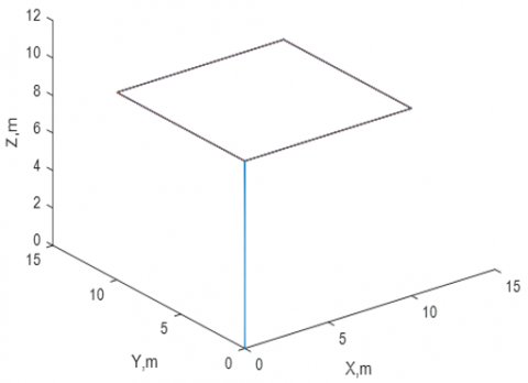
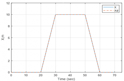
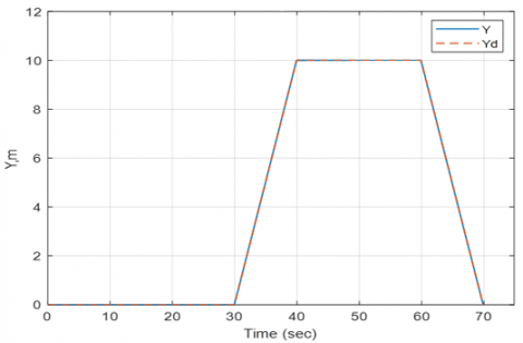
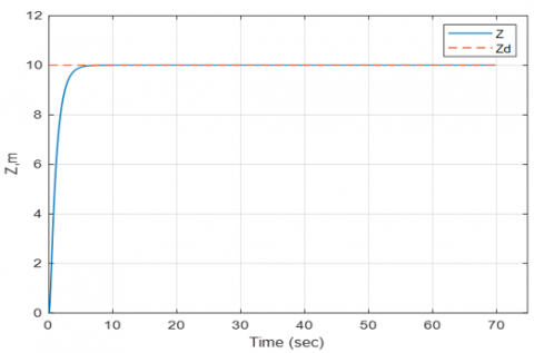
Followed the desired trajectory as when $0<t<20 \mathrm{sec}$., $x_d=0 ; 20<t<30, x_d=t-20 ; 30<t<50, x_d=10$; $50<t<60, x_d=-1(t-50) ; 60<t<70, x_d=0$. When $0<t<30, y_d=0 ; 30<t<40, y_d=t-30 ; 40<$ $t<60, y_d=10 ; 60<t<70, y_d=-1(t-60)$. and when $0<t<70, z_d=10$. The quadrotor flights upward with a fixed path until it reaches a height of $10 \mathrm{~m}$ from the initial positions $(X, Y, Z)=(0,0,0)$.
The simulation results were carried out using MATLAB/Simulink with a time set to 70 sec, As shown in the Figures 5 and 6 below.
Table 4. Firefly algorithm parameters
|
Parameters |
Value |
|
Light absorption coefficient |
1 |
|
Attraction coefficient base value |
1 |
|
Mutation coefficient |
1 |
|
Mutation coefficient damping ratio |
0.98 |
|
Population size |
20 |
|
Iteration max |
40 |
Table 5. Optimal parameters for nonlinear PID
|
Parameter |
Value |
Parameter |
Value |
Parameter |
Value |
|
k11x |
3.0151 |
y3x |
0.01 |
k31y |
1.0242 |
|
k12x |
1.2504 |
a1x |
0.01 |
k32y |
2.5960 |
|
k21x |
4 |
a2x |
0.3450 |
y1y |
1.9688 |
|
k22x |
2.0480 |
a3x |
1.3632 |
y2y |
0.01 |
|
k31x |
0.1105 |
k11y |
4 |
y3y |
3.7522 |
|
k32x |
1.9498 |
k12y |
2.8314 |
a1y |
0.01 |
|
y1x |
2.5793 |
k21y |
3.1710 |
a2y |
1.9894 |
|
y2x |
0.01 |
k22y |
0.01 |
a3y |
0.8624 |
Table 6. Optimal parameters for sliding mode controller
|
Parameters |
Value |
|
k5 |
4 |
|
k6 |
4 |
|
k7 |
3.5165 |
|
k8 |
0.01 |
|
k9 |
0.01 |
|
k10 |
0.01 |
|
k11 |
0.01 |
|
k12 |
0.3410 |
Figure 3. Performance of RMSE using Firefly algorithm
Figure 4. Control of a foldable quadrotor using trapezoidal trajectory
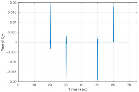
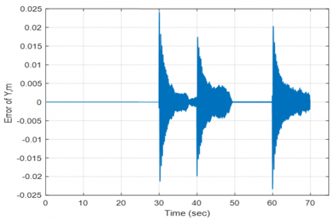
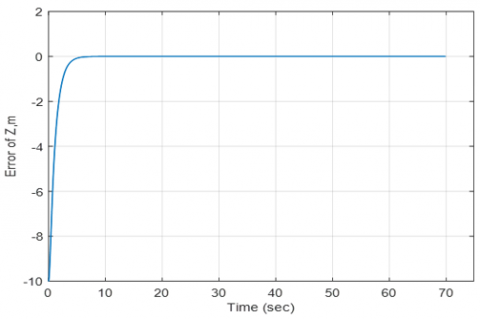
Figures 5 and 6 show the proposed controller's efficiency in ensuring the stability of all possible shapes of the quadrotor while following the proposed path as the error in position approaches zero. Figure 7 shows that the error in the x-axis position varies between 0.02 m to -0.02 m and approaches zero. The error in the y-axis position fluctuates between 0.024 m to -0.024 m and settles at 0.0006686 m.
(a) X trajectory
(b) Y trajectory
(c) Z trajectory
(d) Yaw angle
Figure 5. Response of the position and yaw angle: (a) X trajectory; (b) Y trajectory; (c) Z trajectory; (d) Yaw angle
(a) Tracking error in X position
(b) Tracking error in Y position
(c) Tracking error in Z position
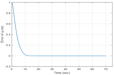
(d) Tracking error in yaw angle
Figure 6. Tracking error in position and yaw angle: (a) Tracking error in X position; (b) Tracking error in Y position; (c) Tracking error in Z position; (d) Tracking error in yaw angle
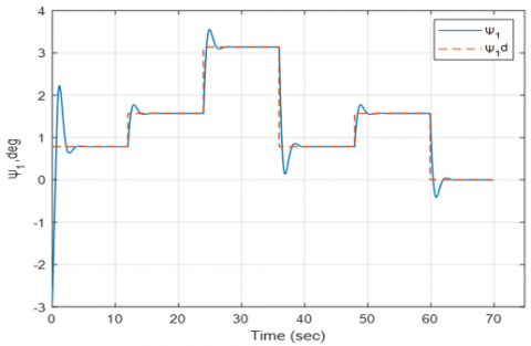
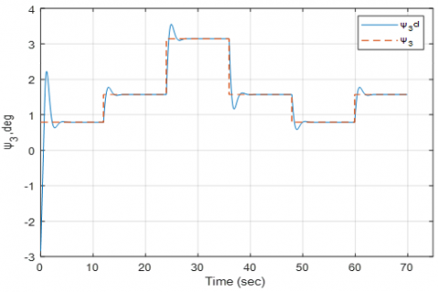
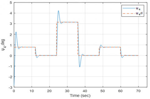
The square shape path, shown in Figure 5, is applied and the quadrotor flights upward with a fixed path until it reaches a height of 5 m from the initial positions (0,0,0). It is noticed from Figure 8 that the quadrotor follows the required path angles with small errors as changed the folded angles every 12 seconds. Using a switch, the foldable angles toggle between these values allowing the quadrotor to change its morphology.
(a) first arm angle ψ1
(b) second arm angle ψ2
(c) third arm angle ψ3
(d) fourth arm angle ψ4
Figure 7. Servomotor's angle variations: (a) first arm angle ψ1; (b) second arm angle ψ2; (c) third arm angle ψ3; (d) fourth arm angle ψ4
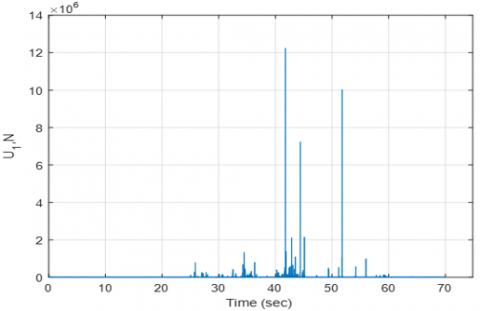
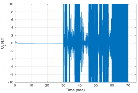
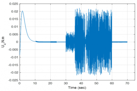
(a) Evolution of the command U1
(b) Evolution of the command U2
(c) Evolution of the command U3
(d) Evolution of the command U4
Figure 8. Control signals. (a) Evolution of the command U1; (b) Evolution of the command U2; (c) Evolution of the command U3; (d) Evolution of the command U4
The value of the control signal U1 changes during the trajectory to reach its highest value after 40 seconds and settles at a fixed value of around 17.76 N. As for the second and third control signals U2, U3, differences appear due to the presence of the multirotor. The fourth control signal U4 takes the highest value at the beginning of the path with the presence of fluctuations and then stabilizes at zero.
This paper presents a proposed architectural control for the foldable quadrotor, known for its complexity and non-linearity, in addition to its high coupling due to the presence of servo motors. Therefore, a control strategy based on the double loop was proposed using two nonlinear controllers (sliding mode control in the inner loop and nonlinear PID in the outer loop). Fireflies algorithm based on the Root Main Square performance indicator was used to improve parameters in each controller.
The proposed controller proved its efficiency in reducing errors in the position and deflection angles and making them close to zero and the controller is suitable for all possible shapes as compared with reference number 13, while maintaining the transit stability of the quadrotor even with the changes its shape.
[1] Chen, T., Shan, J., Liu, H.H.T. (2022). Transportation of payload using multiple quadrotors via rigid connection. International Journal of Aerospace Engineering. https://doi.org/10.1155/2022/2486561
[2] Kadhim, M.Q., Hassan, M.Y. (2020). Design and optimization of backstepping controller applied to autonomous quadrotor. In IOP Conference Series: Materials Science and Engineering, 881(1): 012128. https://doi.org/10.1088/1757-899X/881/1/012128
[3] Muhsen, A., Raafat, S. (2021). Optimized PID control of quadrotor system using extremum seeking algorithm. Engineering and Technology Journal, 39(6): 996-1010. https://doi.org/10.30684/etj.v39i6.1850
[4] Taha, M.Y., Mohamed, M.J., Ucan, O.N. (2020). Optimal 3D path planning for the delivery quadcopters operating in a city airspace. In ISMSIT 2020 - Proceedings of the 4th International Symposium on Multidisciplinary Studies and Innovative Technologies, Istanbul, Turkey, pp. 1-6. https://doi.org/10.1109/ISMSIT50672.2020.9254715
[5] Alawsi, A.A.A., Jasim, B.H., Raafat, S.M. (2020). Improved positioning of delivery quad copter using GPS - accelerometer multimode controller and unscented kalman filter. IOP Conference Series: Materials Science and Engineering, 745(1): 012018. https://doi.org/10.1088/1757-899X/745/1/012018
[6] Derrouaoui, S.H., Bouzid, Y., Guiatni, M., Dib, I., Moudjari, N. (2020). Design and modeling of unconventional quadrotors. In 2020 28th Mediterranean Conference on Control and Automation (MED), Saint-Rapha, France, pp. 721-726. https://doi.org/10.0/Linux-x86_64
[7] Zhao, N., Luo, Y., Deng, H., Shen, Y. (2017). The deformable quad-rotor: Design, kinematics and dynamics characterization, and flight performance validation. In 2017 IEEE/RSJ International Conference on Intelligent Robots and Systems (IROS), Vancouver, BC, Canada, pp. 2391-2396. https://doi.org/10.0/Linux-x86_64
[8] Dilaveroğlu, L., Özcan, O. (2020). Minicore: A miniature, foldable, collision resilient quadcopter. In 2020 3rd IEEE International Conference on Soft Robotics (RoboSoft) New Haven, CT, USA, pp. 176-181. https://doi.org/10.1109/RoboSoft48309.2020.9115993
[9] Kim, S.J., Lee, D.Y., Jung, G.P., Cho, K.J. (2018). An origami-inspired, self-locking robotic arm that can be folded flat. Science Robotics, 3(16): eaar2915. https://doi.org/10.1126/scirobotics.aar2915
[10] Desbiez, A., Expert, F., Boyron, M., Diperi, J., Viollet, S., Ruffier, F. (2017). X-Morf: A crash-separable quadrotor that morfs its X-geometry in flight. In 2017 Workshop on Research, Education and Development of Unmanned Aerial Systems (RED-UAS), Sweden, pp. 222-227. https://doi.org/10.1109/RED-UAS.2017.8101670
[11] Riviere, V., Manecy, A., Viollet, S. (2018). Agile robotic fliers: A morphing-based approach. Soft Robotics, 5(5): 541-553. https://doi.org/10.1089/soro.2017.0120
[12] Yang, D., Mishra, S., Aukes, D.M., Zhang, W. (2019). Design, planning, and control of an origami-inspired foldable quadrotor. In 2019 American Control Conference (ACC), Philadelphia, PA, USA, pp. 2551-2556. https://doi.org/10.23919/ACC.2019.8814351
[13] Falanga, D., Kleber, K., Mintchev, S., Floreano, D., Scaramuzza, D. (2019). The foldable drone: A morphing quadrotor that can squeeze and fly. IEEE Robotics and Automation Letters, 4(2): 209-216. https://doi.org/10.1109/LRA.2018.2885575
[14] Derrouaoui, S.H., Bouzid, Y., Guiatni, M. (2021). PSO based optimal gain scheduling backstepping flight controller design for a transformable quadrotor. Journal of Intelligent and Robotic Systems: Theory and Applications, 102(3): 67. https://doi.org/10.1007/s10846-021-01422-1
[15] Derrouaoui, S.H., Bouzid, Y., Guiatni, M. (2021). Towards a new design with generic modeling and adaptive control of a transformable quadrotor. The Aeronautical Journal, 125(1294): 2169-2199. https://doi.org/10.1017/aer.2021.54
[16] Wissal, T. (2021). Numerical model development of a transformable quadrotor. http://thesis.essa-tlemcen.dz/handle/STDB_UNAM/249.
[17] Majeed, H., Kadhim, S., Jaber, A. (2022). Design of a sliding mode controller for a prosthetic human hand’s finger. Engineering and Technology Journal, 40(1): 257-266. https://doi.org/10.30684/etj.v40i1.1943
[18] Hamoudi, A.K. (2014). Sliding mode controller for nonlinear system based on genetic algorithm. Engineering and Technology Journal, 32(11 Part (A) Engineering).
[19] Najm, A.A., Ibraheem, I.K. (2019). Nonlinear PID controller design for a 6-DOF UAV quadrotor system. Engineering Science and Technology, an International Journal, 22(4), 1087-1097. https://doi.org/10.1016/j.jestch.2019.02.005
[20] Johari, N.F., Zain, A.M., Mustaffa, N.H., Udin, A. (2013). Firefly algorithm for optimization problem. Applied Mechanics and Materials, 421: 512-517. https://doi.org/10.4028/www.scientific.net/AMM.421.512
[21] Wright, H.J., Strydom, R., Srinivasan, M.V. A generalized algorithm for tuning UAS flight controllers. In 2018 International Conference on Unmanned Aircraft Systems (ICUAS), Dallas, TX, USA, pp. 1369-1378. https://doi.org/10.1109/ICUAS.2018.8453451