Salim Al Zerkani*![]() | Yaser Alaiwi
| Yaser Alaiwi![]()
© 2023 IIETA. This article is published by IIETA and is licensed under the CC BY 4.0 license (http://creativecommons.org/licenses/by/4.0/).
OPEN ACCESS
This study investigates heat transfer enhancement through the application of ferro-nanofluid in conjunction with twisted tape inserts, with particular emphasis on the effect of escalating ferro-nanofluid concentration. The influence of a magnetic field on the ferro-nanofluid and its subsequent impact on heat transfer rates is also simulated. To gain a deeper understanding of the stream field, computational fluid dynamics studies are undertaken, with the Cartesian direction being the focal point of mathematical methodologies. The numerical model and mesh are constructed using ANSYS. The numerical results elucidate the heat transfer improvement process utilizing twisted tape and ferro-nanofluid under various conditions: rotational cycles, magnetic field intensity, and ferro-nanofluid concentration. Moreover, the influence of these conditions on pressure, temperature, and fluid velocity is assessed when deploying ferro-nanofluid in conjunction with a magnetic field for heat transfer enhancement. The findings reveal that, irrespective of the operating conditions, fluid pressure tends to decrease while the fluid temperature and velocity increase with the intensification of the magnetic field, the concentration of ferro-nanofluid, and the rotational cycles.
ferro-nanofluid, magnetic field, twisted tube, heat transfer
Several research initiatives will investigate the application of nanofluid more fully in order to enhance its commercialisation. Over the Past ten years, the usage of magnetic nanofluid for enhancing heat transfer has gradually grown because of its superior thermal conductivity compared to other nanofluids. The importance of the research lies in the study of the effect of the magnetic field and the use of an obstructive flow, and this research originality in the simulation process is of little use in previous research. Nanoparticles have a significant impact on the thermal properties of base fluids, such as thermal conductivity and viscosity. When nanofluids are used, the double-tube heat exchanger's ability to transmit heat is considerably enhanced. Other experiments showed that when the concentration of nanofluids was reduced, the heat transfer coefficient increased even more. The using of contemporary electronic devices and anything relevant to the growth that took place in the recent time has recently attracted a lot of curiosity throughout the world. We observe the fascination with heat transfer as a crucial component in several scientific implementations and as having a significant affect many facets of life, such as (optical devices, refrigeration devices, electronics, X-rays, etc.). The miniaturization, data storage, and increased working speed of these electronic gadgets and technologies, together with their massive and quick expansion, created major issues with their heat management [1]. Over the Past few decades, different approaches to improve heat transfer have been advanced. These methods are divided into three groups: I active methods, which involve introducing an external power resource into the fluid (such as electrostatic and mechanical aids domains); (ii) Passive methods, which involve adding fluid additives (such as nanofluids) or turbulence promoters (such as twisted tape and coil inserts); and (iii) compound methods, which involve combining active and passive methods. The first method is by adding motors or obstacles that increase the transfer of thermal energy. The second method is represented by the introduction of active means such as a magnetic field that works to change the movement of the liquid that contains magnetic materials that improve heat transfer. In the third case, the first and second methods are combined [2]. Twisted tapes, dimples, wire coils, fins, ribs, and micro fins have all been used to change the flow Pattern. A flow channel can be modified by changing the thermal characteristics of the working fluid or the fluid flow with the aid of inserts. The working fluid, also known as nanofluid, can be made more efficient by adding nanoparticles with increased thermal conductivity [3]. Super Paramagnetic nanoparticles floating in a nonmagnetic carrier fluid make up magnetic nanofluids, one type of nanofluid. Due to their distinctive properties and behaviour as intelligent or functional fluids, these fluids represent a contemporary collection of nanofluids. Under the effect of an exterior magnetic field, their conductivity and viscosity can alter, and their rheological Parameters can be precisely regulated [4]. A technique for constructing heat transfer devices is to have a larger surface area to volume ratio. For instance, pipes with micro fins have gained popularity due to their capacity to increase the surface of heat transfer and create turbulence in fluid flow. This method might enhance the efficiency of heat transfer [5]. In order to improve the commercialization of nanofluid, several research projects will look into its application more thoroughly. Because magnetic nanofluid has a better thermal conductivity than other nanofluids, its use for improving heat transfer has gradually increased over the Past decade [6]. Base fluids' thermal characteristics, such as thermal conductivity and viscosity, are greatly impacted by nanoparticles. The performance of heat transmission is greatly improved in the double-tube heat exchanger when nanofluids are utilized. According to other studies, the heat transfer coefficient rose even more when the concentration of nanofluids decreased. Additionally, the flow Pattern was connected to how well nanofluids transferred heat. Consequently, additional research was required for the use of nanofluids in plate heat exchangers [7]. A colloidal dispersion of magnetic nanoparticles with a diameter of 3 to 15 nm is called ferrofluid [8]. There are numerous types of Particles with ferromagnetic characteristics, including Fe3O4, CoFeO4, and FePt. This fluid has the property of responding with a magnetic field because of the magnetism of the Particles. The fluid possesses kinetic energy and takes on a Particular shape when a magnetic field is utilized [9]. In other words, there are benefits in that control is achievable with a very basic arrangement and that a flow can only be produced via a magnetic force devoid of direct contact with the fluid. Additionally, it has been demonstrated that because of the characteristics of the Particles, nanofluids perform better thermally than regular fluids [10, 11]. Thermal characteristics of the colloidal suspension are basically different from those of the base fluid. For instance, compared to water or oil, microfluid can have a much better thermal conductivity. The interaction of suspended Particles in multi-component systems like colloidal suspensions has a significant impact on them [12]. The ferrofluid's magnetic property contributes to a well-regulated current, which affects other current physical properties like heat transmission. The colloidal suspension is stabilized by the nanoparticles’ stimulation of repulsion (esterification/ionization) when they are briefly subjected to magnetic fields. By using this technique, van der Waals forces and bipolar contractions that would otherwise cause nanoparticle accumulation and deposition are avoided [13]. New uses for ferrofluid and cutting-edge technologies built around magnetic nanoparticles have arisen over the Past ten years. Examples contain the sensing, energy collecting, and activation of fluid micro magnets, chip-based lab equipment, and specialized medical applications like magnetic hyperthermia, magnetic drug targeting, biomolecule sorting, and magnetic resonance image contrast enhancement. Techniques to improve heat transfer are frequently used in a variety of thermal systems to lower costs, reduce size and weight, and most significantly, improve performance. By disturbing the thermal boundary layer close to the walls and increasing fluid mixing, a swirl flow device can be inserted to improve heat transfer. This will improve convective heat transfer. Nevertheless, the presence of twisted tape inside the tube may result in a greater pressure drop since there is a greater surface area of contact between the fluid and the insert. As a result, scientists have experimented with various twisted tape Patterns and configurations to reduce pressure drops [14, 15]. The velocity profile at the sidewall is changed by the swirl flow created by the twisted tape tube. According to earlier studies, utilizing ribs, fins, baffles, and winglets would provide better thermal performance than using twisted-tape or wire coils [16]. In comparison to stationary twisted tape, self-rotating twisted tape has better thermal presentation. With an increasing in cut length ratio, the Nusselt number increased or heat transfer enhanced. The rectangular cut twisted tape creates a swirl flow that increases fluid mixing and speeds up heat transmission [17]. Transfer of heat in a circular tube is improved via utilizing a conical ring and twisted tape combination in both reverse flow and swirl flow. If 1) the conical ring is used in conjunction with the twisted tape and 2) the twisted tape ratio is low (Y=3.75) to create a larger swirl flow, heat transfer is significantly increased [18]. The Nusselt number or heat transfer enhancement significantly rises because of the improved flow mixing, raising the overall HT coefficient. The existence of the rib increased the rate of HT, according to studies on the thermal efficiency for a square channel with high blocked ribs. The impact of a V-shaped rib on thermofluidic properties for a solar air heater also supported the idea that the design had an impact on how well the device worked. This experiment found that the HT rate greatly improved, resulting in a 2.35-fold increase in hydrothermal performance [19]. The matrix of thermal conductivity and effective flow thermal capacity are both enhanced by the presence of porous media in the flow channel, as is the matrix of porous solids, which enhances radiation heat transfer, especially in two-phase flow (gas-water) systems. According to study, the inclusion of porous media in the flow channel enhances the flow's thermal conductivity matrix and effective heat capacity. In a porous solid-state environment, especially in systems with moving gas, the rate of heat transfer is also accelerated [20]. It is common knowledge that turbulent flow has a higher rate of heat exchange and pumping power than laminar flow, the former of which is desired and the latter undesirable. So, the researchers had the notion to introduce equipment into the laminar flow and induce local turbulence. The concept was a huge hit and is still heavily utilized in the market. This apparatus is known as a tabulator, and up to now, numerous tabulator kinds have been introduced and their performance has been experimentally and quantitatively investigated. Nanostructures have also been used to improve the effectiveness of engineering systems [21]. There are several improvements that can be made to improve the transfer of thermal energy by using magnetic materials because they are materials that do not need energy to be used, but rather use their potential energy.
Computational Fluid Dynamics (CFD) studies are performed to grow a more profound knowledge into the field of the stream. To explain the impact of the disturbance model, (k-ε) model is utilized. Accordingly, the methods of the mathematical arrangement will address these Cartesian direction frameworks (x, y, and z). ANSYS will be utilized to make and network the framework math and afterward to reproduce one case.
2.1 Assumptions
In the current study, water and Fe3O4 is considered as the running nanofluid and the characteristics of flow are assumed (Steady flow, three dimensional, Newtonian, Incompressible, Turbulent).
2.2 Governing equations (magnetic induction method)
In the principal approach, the attractive acceptance condition is gotten from Ohm regulation and Maxwell condition. The condition gives the coupling between the stream field and the attractive field. By and large, Ohm regulation that characterizes this thickness is given by:
$\vec{\jmath}=\sigma \vec{E}$ (1)
where, σ is the electrical conductivity of the media.
For liquid speed field $\vec{U}$ in an attractive field $\vec{B}$, Ohm regulation takes the structure:
$\vec{J}=\sigma(\vec{E}+\vec{U} \times \vec{B})$ (2)
From Ohm regulation and Maxwell condition, the enlistment condition can be inferred as:
$\frac{\partial \vec{B}}{\partial t}+(\vec{U} \cdot \nabla) \vec{B}=\frac{1}{\mu \sigma} \nabla^2 \vec{B}+(\vec{B} \cdot \nabla) \vec{U}$ (3)
From the tackled attractive field $\vec{B}$, the present thickness $\vec{J}$ can be determined involving Ampere's connection as:
$\vec{\jmath}=\frac{1}{\mu} \nabla \times \vec{B}$ (4)
By and large, the attractive field $\vec{B}$ in a MHD issue can be deteriorated into the remotely forced field ($\vec{B}_0$) and the prompted field $\vec{b}$ because of smooth movement. Just the actuated field $\vec{b}$ should be addressed. From Maxwell situations, the forced field $\vec{B}_0$ fulfills the accompanying condition:
$\nabla^2 \vec{B}_0-\mu \sigma^{\prime} \frac{\partial \vec{B}_0}{\partial t}=0$ (5)
where, $\sigma^{\prime}$ is the electrical conductivity of the media wherein field $\vec{B}_0$ is produced. Two cases should be thought of.
2.3 Standard k-$\boldsymbol{\varepsilon}$ model
The standard "k-ε" model (for turbulent kinetic energy and its dissipation rate) is based on model transport equations. The exact equation is used to create the model transport equation for k, while the model transport equation for ε was created through physical reasoning and is not very similar to its mathematically precise cousin. The flow is assumed to be entirely turbulent and the effects of molecular viscosity are insignificant when the k-ε model is derived. Therefore, only totally turbulent flows are suitable for the typical k-ε model. The following transport equations are used to calculate the kinetic energy of the turbulence, k, and its rate of dissipation, ε:
$\begin{aligned} \frac{\partial}{\partial t}(\rho k)+\frac{\partial}{\partial x_i}\left(\rho k u_i\right) = & \frac{\partial}{\partial x_j}\left[\left(\mu+\frac{\mu_t}{\sigma_k}\right) \frac{\partial k}{\partial x_j}\right]+G_k+G_b-\rho \varepsilon -Y_M+S_k\end{aligned}$ (6)
And
$\begin{aligned} \frac{\partial}{\partial t}(\rho \varepsilon)+\frac{\partial}{\partial x_i}\left(\rho \varepsilon u_i\right) & =\frac{\partial}{\partial x_i}\left[\left(\mu+\frac{\mu_t}{\sigma_{\varepsilon}}\right) \frac{\partial \varepsilon}{\partial x_j}\right]+C_{1 \varepsilon} \frac{\varepsilon}{k}\left(G_k+C_{3 \varepsilon} G_b\right) -C_{2 \varepsilon} \rho \frac{\varepsilon^2}{k}+S_{\varepsilon}\end{aligned}$ (7)
In these cases, Gk addresses the age of choppiness active energy due to mean speed slopes, as shown in modeling turbulent production in the k-ε Models. Gb is the age of the disturbance dynamic energy due to lightness, as shown in Effects of Buoyancy on Turbulence in the k-ε Models. YM is concerned with the commitment of the fluctuating dilatation in compressible disturbance to the overall scattering rate, as depicted in Effects of Compressibility on Turbulence in the kε and are the violent Prandtl numbers for k and, respectively. Sk and Sε are client-defined source words. Displaying the Turbulent Viscosity, the violent (or whirlpool) consistency μt is figured by joining k and ε as follows:
$\mu_t=\rho C_\mu \frac{k^2}{\varepsilon}$ (8)
where, Cμ is a constant.
Model Constants The model constants C1ε, C2ε, Cμ, σk, and σε have the following default values:
$C_{1 \varepsilon}=1.44, C_{2 \varepsilon}=1.92, C_\mu=0.09, \sigma_k=1.0, \sigma_{\varepsilon}=1.3$
They have been found to function admirably for a wide scope of divider limited and free shear streams. Albeit the default upsides of the model constants are the standard ones generally broadly acknowledged, you can transform them (if necessary) in the Viscous Model Dialog Box.
2.4 The energy equation
Ansys Fluent solves the energy equation in the following form:
$\begin{aligned} \frac{\partial}{\partial t}\left(\rho\left(e+\frac{v^2}{2}\right)\right)+ & \nabla \cdot\left(\rho v\left(h+\frac{v^2}{2}\right)\right) =\nabla \cdot\left(k_{e f f} \nabla T-\sum_j h_j \vec{J}_j+\tau_{e f f}^{\cdot} \cdot \vec{v}\right) +S_h\end{aligned}$ (9)
where, keff is the forceful conductivity (where ktis the turbulent heat conductivity, as defined by the choppiness model used), and $\vec{J}_j$ is the species j dispersion transition. The first three terms on the right-hand side address energy movement as a result of conduction, species dispersion, and sloppy scattering, in that order. Sh combines the volumetric hotness sources you have identified as well as the hotness aging rate from synthetic replies. Nonetheless, this response source has no effect on the total enthalpy condition (see Energy Sources Due to Reaction for subtleties). The enthalpy h is characterized for ideal gases as:
$h=\sum_j Y_j h_j$ (10)
And for incompressible materials includes the contribution form pressure work.
$h=\sum_j Y_j h_j+\frac{p}{\rho}$ (11)
Yj is the mass fraction of species j and the sensible heat of species hj is the Part of enthalpy that includes only changes in the enthalpy due to specific heat.
$h_j=\int_{T_{r e f}}^T c_{p, j} d T$ (12)
The value used for T ref in the reasonable enthalpy computation is determined by the solver and models employed. T ref is 298.15 K for the tension-based solver, except for PDF models, where Tref is a client input for the species. Tref is 0 for the thickness-based solver, unless when illustrating species movement with responses, in which case T ref is a client input for the species. The internal energy e is uniformly defined for compressible and incompressible materials as:
$e=h-\frac{p_{o p}+p}{\rho}$ (13)
In the above equations, p and pop are check and working strain individually. Such definitions of enthalpy and inward energy oblige an incompressible ideal gas in like manner formulation.
$h=c_v T+\frac{p_{a b s}}{\rho}=c_v T+R_g T+\frac{p}{\rho}=c_p T+\frac{p}{\rho}$ (14)
2.5 The mass conservation equation
The mass conservation equation, often known as the continuity equation, is written as follows:
$\frac{\partial \rho}{\partial t}+\nabla \cdot(\rho \vec{v})=S_m$ (15)
This is the most general sort of mass protection condition, and it applies to both incompressible and compressible streams. The mass contributed to the persistent stage from the scattered second stage (for example, due to evaporation of fluid droplets) and any client-defined sources is called Sm. For 2D axisymmetric calculations, the progression condition is given by:
$\frac{\partial \rho}{\partial t}+\frac{\partial}{\partial x}\left(\rho v_x\right)+\frac{\partial}{\partial r}\left(\rho v_r\right)+\frac{\rho v_r}{r}=S_m$ (16)
where, x is the axial coordinate, r is the radial coordinate, vX is the axial velocity, and vr is the radial velocity.
2.6 Momentum conservation equations
In an inertial (non-accelerating) reference frame, momentum is conserved.
$\frac{\partial}{\partial t}(\rho \vec{v})+\nabla \cdot(\rho \vec{v} \vec{v})=-\nabla p+\nabla \cdot\left(\underline{\tau^{-}}\right)+\rho \vec{g}+\vec{F}$ (17)
where, p denotes the static strain, tensor denotes the pressure tensor (shown below), and g and F denote the gravitational and outer body powers, respectively (for example, those arising from interaction with the scattering stage). Other model-subordinate source terminology, such as permeable media and client described sources, are also included in F. The pressure tensor $\underline{\tau^{-}}$ is given by:
$\underline{\tau^{-}}=\mu\left[\left(\nabla \vec{v}+\nabla \vec{v}^T\right)-\frac{2}{3} \nabla \cdot \vec{v} I\right]$ (18)
where the subatomic thickness is small and the influence of volume widening is the second component on the right-hand side. The pivotal and spiral force protection criteria for 2D axisymmetric computations are given by:
$\begin{aligned} \frac{\partial}{\partial t}\left(\rho v_x\right)+\frac{1}{r} \frac{\partial}{\partial x}\left(r \rho v_x v_x\right)+\frac{1}{r} \frac{\partial}{\partial r}\left(r \rho v_r v_x\right) =-\frac{\partial p}{\partial x} +\frac{1}{r} \frac{\partial}{\partial x}\left[r \mu\left(2 \frac{\partial v_x}{\partial x}-\frac{2}{3}(\nabla \cdot \vec{v})\right)\right] +\frac{1}{r} \frac{\partial}{\partial r}\left[r \mu\left(\frac{\partial v_x}{\partial r}+\frac{\partial v_r}{\partial x}\right)\right]+F_x\end{aligned}$ (19)
And
$\begin{aligned} \frac{\partial}{\partial t}\left(\rho v_r\right)+\frac{1}{r} \frac{\partial}{\partial x}\left(r \rho v_x v_r\right)+\frac{1}{r} \frac{\partial}{\partial r}\left(r \rho v_r v_r\right) =-\frac{\partial p}{\partial r}+\frac{1}{r} \frac{\partial}{\partial x}\left[r \mu\left(\frac{\partial v_r}{\partial x}+\frac{\partial v_x}{\partial r}\right)\right] +\frac{1}{r} \frac{\partial}{\partial r}\left[r \mu\left(2 \frac{\partial v_r}{\partial r}-\frac{2}{3}(\nabla \cdot \vec{v})\right)\right] -2 \mu \frac{v_r}{r^2}+\frac{2}{3} \frac{\mu}{r}(\nabla \cdot \vec{v})+\rho \frac{v_z^2}{r}+F_r\end{aligned}$ (20)
where,
$\cdot \vec{v}=\frac{\partial v_x}{\partial x}+\frac{\partial v_r}{\partial r}+\frac{v_r}{r}$ (21)
And vz is the swirl velocity.
2.7 Turbulence model
The average (k-ε) model is efficient with consistent exactness for wide violent streams reach and it is by and large utilized in the reproduction of hotness move. In the (k-ε) model, two extra transport equations for the tempestuous motor energy (k) and violent dispersal rate (ε) are addressed and the whirlpool consistency (μt) is figured as an element of k and ε.
The (k-ε) model is a turbulence model commonly used in computational fluid dynamics (CFD) simulations to predict turbulent flows. It provides a closure model for the Reynolds-averaged Navier-Stokes (RANS) equations by introducing two additional transport equations for the turbulent kinetic energy (k) and the turbulent dissipation rate (ε). The purpose of the (k-ε) model is to provide closure to the RANS equations by modeling the effects of turbulence on the mean flow. By solving the transport equations for k and ε, the model allows for the prediction of turbulence quantities, which in turn affect the flow behavior, such as velocity fluctuations, turbulence intensity, and eddy viscosity. It's important to note that the specific coefficients and model constants used in the (k-ε) model may vary depending on the implementation or specific version of the model being used. The equations provided here represent the general form of the (k-ε) model.
2.8 ANSYS package
The stream conditions are addressed by utilizing two modules:
1- The essential module is pre-processor module; a program structure that makes the calculation and matrix as in the accompanying:
a) Modelling of calculation.
b) Mesh age.
c) Boundary condition.
2- The second module is the Solution module, for settling Navier-Stokes conditions (which incorporates progression, force and energy conditions), as well as the violent stream model.
2.9 System geometry
The system engineering system is shown in Figure 1. Where the model was designed with an internal diameter of 25.4 mm for flow and a total length of the tube 500 mm and contains within it a twisted bar with a thickness of 2 mm and a length of 20 mm. Where three values of the torsion rotation are taken once two, four and six turns, and it will also be shed Magnetic field with different tolerances, where the length of the magnetic field was taken once 30 mm, 50 mm and 70 mm. To obtain a model that can be applied in reality and is feasible to facilitate the work of researchers in the future.
Figure 1. Geometry shape
2.10 Mesh generation
Generally, because unstructured grids work well for complicated geometries, the unstructured tetrahedron grids were chosen in the current investigation. ANSYS support solid geometry mesh generation and three-dimensional models with minimum input from a single phase from the user. The number of cells taken, in this study was (2223270), see Figure 2.
In order to obtain accurate and reliable results, a Mesh independency must be made to see the clear change when changing the number of the element and the output results, as it stops when the stability of the output results is reached, where the element size is used 0.001m as shown in Table 1.
2.11 Conditions of the boundary
Figure 3 shows the limits that were used, where three variable entry velocities were taken at the entry area (0.1, 0.3, and 0.5) m/s representing the entry of the nanomaterial at a temperature of 25℃. In the exit area, an exit pressure of 0 Pa was applied to the surfaces of Heat A constant temperature of 40 C was shed, where three cases of the magnet were taken when the magnet have length 30, 50, 70 mm, then the twisted tape have 2 turns ,4 turns and 6 turns. Three forces of magnetic flux were taken (2, 4 and 6) tesla.
Figure 2. Mesh generated by ANSYS
Figure 3. Boundary of conditions
2.12 Problem solution
A volume of the control depended technique that comprises of the accompanying advances, which can be utilized for arrangement:
• A mesh is created on the field.
• Sets of conditions like velocity, pressure, and preserved scalars, mathematical are built by the combination on each control volume of the administering conditions.
•The Discretized Equations are linearized and tackled iteratively.
Table 1. Mesh independency
|
Case |
Node |
Element |
Max. Temperature (K) |
Outlet Temperature (K) |
Pressure Difference (Pa) |
|
1 |
252360 |
1253477 |
335.812 |
305.363 |
47.42 |
|
2 |
326252 |
1532207 |
331.493 |
302.976 |
49.21 |
|
3 |
483412 |
1744345 |
329.081 |
302.881 |
49.47 |
|
4 |
597355 |
2223270 |
329.074 |
302.879 |
49.48 |
ANSYS is the arrangement calculation utilized by FLUENT and is embraced in the current work. The overseeing conditions are settled consecutively (i.e., isolated from each other). Since the administering conditions are non-straight (and coupled), numerous cycles might be done before a joined arrangement is gotten as shown in Figure 4.
Figure 4. Flow chart of CFD
2.13 Solution parameters
The solution parameters include the following:
A. Precision Solver Type
Ordinarily, accuracy solvers are found by single and twofold as it were. A PC with limitless accuracy, residuals would go to zero as the arrangement combines. A genuine PC, the residuals rot to some little worth ("adjust") and afterward end changing ("level out").
B. Iterations Number
This is the highest digit of iterations done before the solver terminates.
Analyzing the solution complexity of a problem involves assessing the computational resources required to solve the problem accurately and efficiently. The optimal solution, in this case, would aim to strike a balance between accuracy and computational efficiency. Here are a few factors to consider: 1- Grid Resolution: Increasing the grid resolution leads to more accurate results but also increases computational cost. The optimal solution should determine an appropriate grid resolution that captures the essential features of the flow without excessive refinement. 2- Turbulence Model Selection: The (k-ε) model is a relatively simple turbulence model, but more advanced models like Reynolds Stress Models (RSM) or Large Eddy Simulation (LES) can provide better accuracy at the expense of increased computational complexity. The optimal solution should consider the trade-off between accuracy and computational cost and select an appropriate turbulence model based on the specific requirements of the problem. 3- Numerical Methods: The choice of numerical methods for solving the governing equations can impact computational efficiency. Different methods like finite difference, finite volume, or finite element methods have varying levels of complexity and accuracy. The optimal solution should identify the most suitable numerical method that balances accuracy and computational cost. 4- Parallel Computing: Taking advantage of parallel computing techniques, such as utilizing multiple processors or distributed computing, can significantly reduce the computational time for solving complex problems. The optimal solution should explore parallel computing strategies to improve the computational efficiency, especially for large-scale simulations. 5- Model Calibration and Validation: The accuracy of the turbulence model heavily relies on appropriate calibration and validation against experimental or high-fidelity simulation data. The optimal solution should include a thorough calibration and validation process to ensure the model's accuracy within an acceptable range, minimizing the need for excessive computational resources. In summary, the optimal solution for analyzing the solution complexity of the problem and achieving accurate results with the (k-ε) model involves carefully selecting appropriate grid resolution, turbulence model, numerical methods, and parallel computing techniques. It should also involve model calibration and validation to ensure the model's accuracy while minimizing computational resources.
2.14 Convergence criteria
The CFD method requires emphasizing the arrangement of the liquid stream conditions till it is met. The emphases are halted when the arrangement continues as before inside the exactness of the chose intermingling models. The most generally utilized strategy to check arrangement combination is the mistake residuals, which is the contrast between the upsides of a variable in two continuous emphases standardized by the biggest outright leftover for the initial five cycles. The arrangement is supposed to be united when the residuals are under a resilience breaking point of 10-6 for all the liquid stream conditions introduced previously.
3.1 Effect of cycles of rotation
Cycles of rotation is one of the influential factors in enhancement in heat transfer, which play an important role. Figures 5 and 6 explain the effect of cycles of rotation on the enhance heat transfer rate. From these figures it has been noticed that when cycle of rotation is 2 cycles, intensity of magnetic field is 6 Tesla, and concentration 0.5 wt.%. The effect of cycles on the pressure of fluid decreased from 351.782 to -13.5 Pa at 30 mm width of magnetic field. In addition, at 50 mm width of magnetic field, the pressure still decreased from 414.584 to -11.627 Pa.
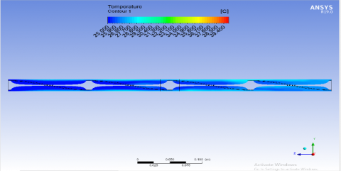
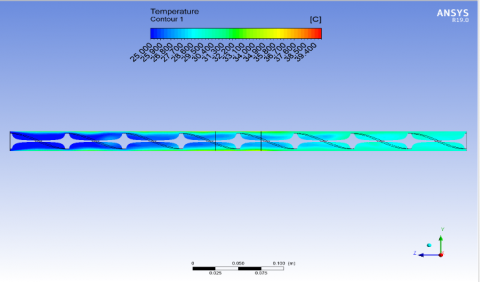
The effect of cycles on the temperature of fluid have been displayed in Figures 7 and 8, it can be concluded that the temperature increased from 25.0 to 39.4℃ at 2 cycles, 6 Tesla intensity of magnetic field, and 0.5 wt.% concentration of ferro-nanofluid with 30 mm width of magnetic field. At 50 mm width of magnetic field, the temperature of fluid raised from 25.0 to 39.4℃ at 2, 6, and 0.5 of cycles of rotation, intensity of magnetic field, and concentration of ferro-nanofluid respectively.
Figure 5. Effect of cycles of rotation on pressure of fluid at 2 cycles, 0.5 wt. % concentration of ferro-nanofluid, and 6 Tesla intensity of magnetic field with 30 mm width of magnetic field
Figure 6. Effect of cycles of rotation on pressure of fluid at 2 cycles, 0.5 wt.% concentration of ferro-nanofluid, and 6 Tesla intensity of magnetic field with 50 mm width of magnetic field
Figure 7. Effect of cycles of rotation on temperature of fluid at 2 cycles, 0.5 wt. % concentration of ferro-nanofluid, and 6 Tesla intensity of magnetic field with 30 mm width of magnetic field
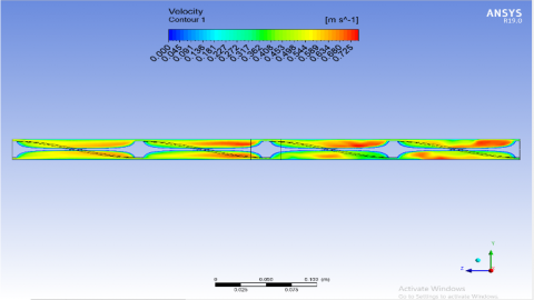
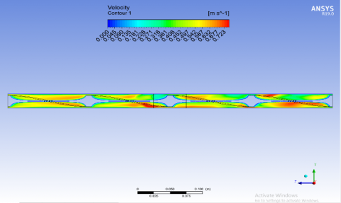
Figures 9 and 10 show the effect of cycles of rotation on the velocity of fluid. The velocity of fluid tends to grow from 0.0 to 0.725 m/s at condition of 2 cycles, intensity of magnetic field 6 Tesla, and concentration of ferro-nanofluid is 0.5 wt.% with 30 mm width of magnetic field. The similar outcomes of velocity of fluid appeared at the same conditions with 50 mm width of magnetic field whereas velocity increased from 0.0 to 0.723 m/s.
The twisted tape inserts act as Passive turbulence promoters in an effort to increase heat transfer rates. The inclusion of these inserts causes the flow to experience the following benefits: I higher local velocities due to the reduced flow area, which is accompanied by secondary flow recirculation; (ii) improved mixing and turbulence by the helically twisted fluid flow; and (iii) improved heat transfer in the flow because the inserts act as fins. The heat transfer rate rises as a result of these interrelated factors. The implants' only real drawback is the little increase in pumping force needed to compensate for the pressure decrease they create. Additionally, it can be seen that the magnetic field has very little influence on the pressure drop. When an external force is present, pressure drops rise. The fundamental reason viscosity increases in the presence of an external magnetic field is pressure decrease. Additionally, the development of vortices that serve as barriers in the flow field may also be a factor in the second explanation for the rise in pressure drop. When a magnetic dipole source is used to create the magnetic field, this is what happens. The recent findings, however, were based on the supposition that viscosity is solely a product of temperature and concentration. Additionally, the heated ferrofluid tends to be removed off the surface by the upward magnetic force without the development of a vortex. Therefore, there has not been a significant change in the pressure decrease because of the magnetic field.
Figure 8. Effect of cycles of rotation on temperature of fluid at 2 cycles, 0.5 wt.% concentration of ferro-nanofluid, and 6 Tesla intensity of magnetic field with 50 mm width of magnetic field
Figure 9. Effect of cycles of rotation on velocity of fluid at 2 cycles, 0.5 wt. % concentration of ferro-nanofluid, and 6 Tesla intensity of magnetic field with 30 mm width of magnetic field
The pressure drop increases when velocity of fluid rises from 0.1 to 0.5 m/s. At thickness of magnetic 30 mm, 2 cycles of rotation, and intensity of magnetic 2 Tesla, the pressure drop reach to 35 Pa with 0.1 m/s. While at 0.3 and 0.5 m/s, pressure drop record 154.8 Pa, and 339.2 respectively with the same other operating conditions as shown in Figure 11.
Figure 10. Effect of cycles of rotation on velocity of fluid at 2 cycles, 0.5 wt. % concentration of ferro-nanofluid, and 6 Tesla intensity of magnetic field with 50 mm width of magnetic field
Figure 11. Effect of cycles of rotation and intensity of magnetic field on pressure drop at velocity 0.1 m/s and thickness of magnetic 30 mm
Figure 12. Effect of concentration of ferro-nanofluid on pressure of fluid at 4 cycles, 0.1 wt. % concentration of ferro-nanofluid, and 4 Tesla intensity of magnetic field with 30 mm width of magnetic field
3.2 Effect of concentration of ferro-nanofluid
Concentration of ferro-nanofluid is one of the most important Parameter, which has effect on the pressure, temperature, and velocity of fluid. Figures 12 and 13 show the effect of concentration on the pressure of a fluid. As mentioned in the previous sections, pressure of fluid decrease from 38.276 to -0.629 Pa, and 36.647 to -0.645 Pa for 30 mm, and 50 mm of magnetic field respectively with 4 cycles of rotation, 4 Tesla intensity of magnetic field, and 0.1 wt.% concentration of ferro-nanofluid.
Temperature of fluid rise at the similar level from 25 to 39. 4℃ with 30 mm, and 50 mm width of magnetic field at 0.1 wt.% concentration of ferro-nanofluid, 4 cycles of rotation, and 4 Tesla intensity of magnetic field as shown in Figures 14 and 15.
Figure 13. Effect of concentration of ferro-nanofluid on pressure of fluid at 4 cycles, 0.1 wt. % concentration of ferro-nanofluid, and 4 Tesla intensity of magnetic field with 50 mm width of magnetic field
Figure 14. Effect of concentration of ferro-nanofluid on temperature of fluid at 4 cycles, 0.1 wt. % concentration of ferro-nanofluid, and 4 Tesla intensity of magnetic field with 30 mm width of magnetic field
Figure 15. Effect of concentration of ferro-nanofluid on temperature of fluid at 4 cycles, 0.1 wt. % concentration of ferro-nanofluid, and 4 Tesla intensity of magnetic field with 50 mm width of magnetic field
While the velocity of fluid increase from 0.009 to 0.146 m/s, and from 0.01 to 0.155 m/s at 30 mm, and 50 mm width of magnetic field respectively, with 0.1 wt.% concentration of ferro-nanofluid, 4 cycles of rotation, and 4 Tesla intensity of magnetic field, see Figures 16 and 17.
Figure 16. Effect of concentration of ferro-nanofluid on velocity of fluid at 4 cycles, 0.1 wt. % concentration of ferro-nanofluid, and 4 Tesla intensity of magnetic field with 30 mm width of magnetic field
Figure 17. Effect of concentration of ferro-nanofluid on velocity of fluid at 4 cycles, 0.1 wt. % concentration of ferro-nanofluid, and 4 Tesla intensity of magnetic field with 50 mm width of magnetic field
The magnetic dipoles of the ferromagnetic particles are aligned with the magnetic field's lines and are magnetized particles. Due to the strong Kelvin force present, ferrofluid particles that are rotating close to the magnetic source deviate as a result. The magnetization of nanoparticle, which decreases at the bottom wall at high temperatures, can be used to explain this rotating action. Due to the thermomigration phenomena, the warm ferrofluid near the bottom wall travels to the colder areas where its magnetization rises. Therefore, the creation of the recirculation zone is caused by the non-uniformity of the magnetization of nanoparticles. This behaviour becomes more noticeable and the recirculation zone gets hotter as the magnetic field strength rises. The related temperature fields show the presence of a thermal boundary layer close to the heated wall, where parallel isotherms show that conduction heat transfer is the dominant mechanism of heat transfer. Applying and enhancing the magnetic field disturbs this property of the thermal layer. In fact, due to the movement of ferrofluid under the influence of the thermodiffusion phenomena, the isotherms become distorted in the recirculation zone and demonstrate the dominance of the convective heat transfer mode. By raising the magnetic number, the isotherms downstream of recirculation become narrower. This is because the heated wall was affected by the downward main flow distortion following recirculation. Due to this fact, the local heat transfer rate and temperature gradient both rise. It is challenging to establish the changes in velocity together with the changes in nanoparticle concentration since the density and viscosity rise with increasing nanoparticle concentration. Numbers are used to study the connection between velocity and nanoparticle concentration. Maxwell's theory states that as the Reynolds number (or flow rate) and nanoparticle concentration increase, the pressure drop in the tube rises, increasing energy consumption and decreasing experiment efficiency. Studying how the resistance coefficient varies with flow rate and nanoparticle mass percentage is essential. In fluid mechanics, the resistance coefficient is a dimensionless quantity. It is used to show that the shape of the tube (twisted tape) and the properties of the nanofluids mostly influence the resistance of nanofluids in a tube.
The pressure drop reach to 37.5, 36.6, and 37.8 Pa at intensity of magnetic field 2, 4, and 6 Tesla, and 4 cycles of rotation respectively, with 50 mm thickness of magnetic, and 0.1 m/s. Figure 18 shows the behavior of pressure drop.
Figure 18. Effect of cycles of rotation and intensity of magnetic field on pressure drop at velocity 0.1 m/s and thickness of magnetic 50 mm
Figure 19. Effect of intensity of magnetic field on pressure of fluid at 2 cycles of rotation, 0.1 wt. % concentration of ferro-nanofluid, and 2 Tesla intensity of magnetic field with 30 mm width of magnetic field
3.3 Effect of intensity of magnetic field
The factor of intensity of magnetic field has been investigated to explain the effect of magnetic field on pressure, temperature, and velocity of fluid. The pressure going to drop at 2 Tesla intensity of magnetic field, 2 cycles of rotation, and 0.1 wt.% concentration of ferro-nanofluid. Figures 19 and 20 shows the pressure decrease from 35.044 to -0.094 Pa, and from 31.977 to -0.038 at 30 mm, and 50 mm width of magnetic field respectively.
The same rising of temperature has been obtained for all widths of magnetic field with 2 cycles of rotation, 2 Tesla intensity of magnetic field, and 0.1 wt. % concentration of ferro-nanofluid, see Figures 21 to 22.
Figure 20. Effect of intensity of magnetic field on pressure of fluid at 2 cycles of rotation, 0.1 wt. % concentration of ferro-nanofluid, and 2 Tesla intensity of magnetic field with 50 mm width of magnetic field
Figure 21. Effect of intensity of magnetic field on temperature of fluid at 2 cycles of rotation, 0.1 wt. % concentration of ferro-nanofluid, and 2 Tesla intensity of magnetic field with 30 mm width of magnetic field
Figure 22. Effect of intensity of magnetic field on temperature of fluid at 2 cycles of rotation, 0.1 wt. % concentration of ferro-nanofluid, and 2 Tesla intensity of magnetic field with 50 mm width of magnetic field
Figures 23 and 24 present the effect of intensity of magnetic field on velocity of fluid. It is clear that the velocity grows from 0.009 to 0.148 m/s with 30 mm width of magnetic field, and continues to increase with 50 mm width of magnetic field at 2 cycles of rotation, 2 Tesla intensity of magnetic field, and 0.1 wt. % concentration of ferro-nanofluid.
Figure 23. Effect of intensity of magnetic field on velocity of fluid at 2 cycles of rotation, 0.1 wt. % concentration of ferro-nanofluid, and 2 Tesla intensity of magnetic field with 30 mm width of magnetic field
Figure 24. Effect of intensity of magnetic field on velocity of fluid at 2 cycles of rotation, 0.1 wt. % concentration of ferro-nanofluid, and 2 Tesla intensity of magnetic field with 50 mm width of magnetic field
It can be seen that the heat transfer rate, exhibits similar patterns and rises with increasing magnetic field strength at each constant centration. Additionally, a significant increase in the heat transfer is shown in the presence of a magnetic field compared to both the absence of a magnetic field and water as the base fluid, respectively. This could be because of the chain-like structures that were created in the magnetic fields that were applied, which enhanced the convective heat transfer coefficient. Magnetic moments tended to line up with the applied magnetic field when there was an applied magnetic field present. When magnetic nanoparticle was mostly influenced by magnetic force as opposed to thermal motion. The nanoparticles produced chains that were orientated in the same direction as the applied field and stuck together. As a result, the chains connecting the flow of nanofluids and the pipe wall function as thermal tunnels, improving heat transfer. With the use of a steady magnetic field without any pumping power, the enhancement of heat transfer improves. This is due to the fact that when a steady magnetic field is supplied, the ferrofluid's dipoles align in the same direction as the magnetic field's applied externally, leading to a higher rate of heat transfer than would otherwise occur in the absence of a magnetic field.
The behavior of pressure drop still the same as mentioned above, ΔP increase to 44.9, 44.8, and 44.9 Pa at 2, 4, and 6 Tesla intensity of magnetic field respectively. Figure 25 display the growing of pressure drop at 2, 4, and 6 cycles of rotation respectively, with 70 mm thickness of magnetic.
Figure 25. Effect of cycles of rotation and intensity of magnetic field on pressure drop at velocity 0.1 m/s and thickness of magnetic 70 mm
From the current research, the following findings may be drawn:
1) Fe3O4 nanofluid was used in an investigation to examine heat transfer. It was found that heat transfer increased significantly with Reynolds number or flow rate, and the base fluid's heat transport was partially improved by the addition of nanoparticles. The use of ferro-nanofluid and magnetic field was successful and very efficient.
2) Computational Fluid Dynamics (CFD) studies are conducted to gain a deeper understanding of the field of the stream. The k-e model is used to explain the impact of the disturbance model. Water and Fe3O4 are considered as the running nanofluid and the characteristics of flow are assumed (Steady, Three dimensional, Newtonian, Incompressible, Turbulent).
3) Ferrofluid's secondary magneto convective flow in the direction of the permanent magnet results in a reduction in convective heat transfer. However, when the flow rate is increased, convective heat transfer and Nu number are enhanced. This phenomenon was fully simulated, taking into account the movement of mass, heat, and momentum in the system. The simulation findings are in good agreement with experimental data, and can be used to design heat transfer devices for many uses, such as cooling electronics and micro reactors.
4) The parameters of concentration of ferro-nanofluid, intensity of magnetic field, and cycles of rotation have been taken into account to explain the effect on pressure, temperature, and velocity of fluid. Pressure decreases with increased intensity, while temperature and velocity rise with increased intensity.
[1] Khalaf, A.F., Basem, A., Hussein, H.Q., Jasim, A.K., Hammoodi, K.A., Al-Tajer, A.M., Omer, I., Flayyih, M.A. (2022). Improvement of heat transfer by using porous media, nanofluid, and fins: A review. International Journal of Heat and Technology, 40(2): 497-521. https://doi.org/10.18280/ijht.400218
[2] Mashayekhi, R., Arasteh, H., Talebizadehsardari, P., Kumar, A., Hangi, M., Rahbari, A. (2021). Heat transfer enhancement of nanofluid flow in a tube equipped with rotating twisted tape inserts: A two-phase approach. Heat Transfer Engineering, 43(7): 608-622. https://doi.org/10.1080/01457632.2021.1896835
[3] Ahmad, S., Abdullah, S., Sopian, K. (2020). A review on the thermal performance of nanofluid inside circular tube with twisted tape inserts. Advances in Mechanical Engineering, 12: 1-26. https://doi.org/10.1177/1687814020924893
[4] Ghadiri, M., Haghani, O., Emam-jomeh, E., Barati, E. (2021). Experimental investigation on laminar convective heat transfer of ferro-nanofluids under constant and alternating magnetic field. AUT Journal of Mechanical Engineering, 5(3): 477-494. https://doi.org/10.22060/ajme.2020.18628.5908
[5] Kristiawan, B., Wijayanta, A.T., Enoki, K., Miyazaki, T., Aziz, M. (2019). Heat transfer enhancement of TiO2/water nanofluids flowing inside a square Minichannel with a Microfin structure: A numerical investigation. Energies, 12(16): 3041. https://doi.org/10.3390/en12163041
[6] Bhattacharyya, S., Vishwakarma, D.K., Roy, S., Dey, K., Benim, A.C., Bennacer, R., Paul, A.R., Huan, Z. (2021). Computational investigation on heat transfer augmentation of a circular tube with novel hybrid ribe. E3S Web of Conferences, 321: 04012. https://doi.org/10.1051/e3sconf/202132104012
[7] Jiawang, Y., Xian, Y., Jin, W., Hon, H., Bengt, S. (2022). Review on thermal performance of nanofluids with and without magnetic fields in heat exchange devices. Frontiers in Energy, 10.
[8] Ellahi, R., Tariqb, M., Hassanc, M., Vaf, K. (2016). On boundary layer nano-ferroliquid flow under the influence of low oscillating stretchable rotating disk. Journal of Molecular Liquids, 229: 339-345. https://doi.org/10.1016/j.molliq.2016.12.073
[9] Sheikhnejad, Y., Hosseini, R., Avval, M.S. (2016). Experimental study on heat transfer enhancement of laminar ferrofluid flow in horizontal tube Partially filled porous media under fixed Parallel magnet bars. Journal of Magnetism and Magnetic Materials, 424: 16-25. https://doi.org/10.1016/j.jmmm.2016.09.098
[10] Kristiawan, B., Santoso, B., Wijayanta, A.T., Aziz, M., Miyazaki, T. (2018). Heat transfer enhancement of TiO2/water nanofluid at laminar and turbulent flows: A numerical approach for evaluating the effect of nanoparticle loadings. Energies, 11(6): 1584. https://doi.org/10.3390/en11061584
[11] Mutar, W.M., Alaiwi, Y. (2023). Experimental investigation of thermal performance of single pass solar collector using high porosity metal foams. Case Studies in Thermal Engineering, 45: 102879. https://doi.org/10.1016/j.csite.2023.102879
[12] Cherepanov, I.N., Krauzin, P.V. (2019). On the thermodynamic theory of colloidal suspensions. Physica A: Statistical Mechanics and Its Applications, 540: 123247. https://doi.org/10.1016/j.physa.2019.123247
[13] Khan, W.A., Khan, Z.H., Haq, R.U. (2015). Flow and heat transfer of ferrofluids over a flat plate with uniform heat flux. The European Physical Journal Plus, 130: 86. https://doi.org/10.1140/epjp/i2015-15086-4
[14] Bezaatpour, M., Goharkhah, M. (2019). Effect of magnetic field on the hydrodynamic and heat transfer of magnetite ferrofluid flow in a porous fin heat sink. Journal of Magnetism and Magnetic Materials, 476: 506-515. https://doi.org/10.1016/j.jmmm.2019.01.028
[15] Ahmad, S., Abdullah, S., Sopian, K. (2020). A review on the thermal performance of nanofluid inside circular tube with twisted tape inserts. Advances in Mechanical Engineering, 12: 1-26. https://doi.org/10.1177/1687814020924
[16] Skullong, S., Thianpong, C., Jayranaiwachira, N., Promvonge, P. (2019). Experimental and numerical heat transfer investigation in turbulent square-duct flow through oblique horseshoe baffles. Chemical Engineering and Processing, 90: 58-71. https://doi.org/10.1016/j.cep.2015.11.008
[17] Paneliya, S., Khanna, S., Mankad, V., Ray, A., Prajapati, P., Mukhopadhyay, I. (2020). Comparative study of heat transfer characteristics of a tube equipped with X-shaped and twisted tape insert. Materials Today: Proceedings, 28(Part 2): 1175-1180. https://doi.org/10.1016/j.matpr.2020.01.103
[18] Promvonge, P., Eiamsa-ard, S. (2007). Heat transfer behaviors in a tube with combined conical-ring and twisted-tape insert. International Communications in Heat and Mass Transfer, 34(7): 849-859. https://doi.org/10.1016/j.icheatmasstransfer.2007.03.019
[19] Olabi, A.G., Wilberforce, T., Sayed, E.T., Elsaid, K., Atiqure Rahman, S.M., Abdelkareem, M.A. (2021). Geometrical effect coupled with nanofluid on heat transfer enhancement in heat exchangers. International Journal of Thermofluids, 10: 100072. https://doi.org/10.1016/j.ijft.2021.100072
[20] Al-Aloosi, W., Alaiwi, Y., Hamzah, H. (2023). Thermal performance analysis in a parabolic trough solar collector with a novel design of inserted fins. Case Studies in Thermal Engineering, 49: 103378.https://doi.org/10.1016/j.csite.2023.103378
[21] Yang, L., Baghaei, S., Suksatan, W., Barnoon, P., Sharma, S., Davidyants, A., El-Shafay, A.S. (2022). Numerical assessment of the influence of helical baffle on the hydrothermal aspects of nanofuid turbulent forced convection inside a heat exchanger. Scientific Reports, 12: 2245. https://doi.org/10.1038/s41598-022-06049-2