Robert Kosova*![]() | Evgjeni Xhafaj
| Evgjeni Xhafaj![]() | Daniela Halidini Qendraj
| Daniela Halidini Qendraj![]() | Irakli Prifti
| Irakli Prifti
© 2023 IIETA. This article is published by IIETA and is licensed under the CC BY 4.0 license (http://creativecommons.org/licenses/by/4.0/).
OPEN ACCESS
The Hubbert curve model has been foundational in the representation and analysis of historical oil production data since its inception in the 1950s. Its prestige was further bolstered following the successful prediction of peak oil in the United States in the 1970s. This model has proven its efficacy in encapsulating production trends for finite and non-renewable resources, including hydrocarbons and various minerals. Its utility extends to the evaluation of disparate scales of production, from individual wells to expansive oil fields and entire regions. In the present study, the historical oil production data from Albania is scrutinized, and several growth functions, such as the Logistic and Gaussian, are tested for their appropriateness in portraying this data. The consequent analysis of the tested models indicates that the oil production curve for Albania is monocyclic and exhibits asymmetry. This in-depth exploration of potential growth functions underscores the enduring relevance of the Hubbert curve model in understanding patterns in fossil fuel production.
Hubbert, curve, math modelling, oil production, Albania
Several methodologies have been developed to represent and forecast oil production curves for oilfields, regions, and countries. These methodologies are primarily categorized into three distinct approaches: economic, geophysical, and hybrid. The economic approach relies on factors like oil prices, costs, regulations, and other variables to elucidate oil production and supply. Conversely, the geophysical approach typically employs curve-fitting models, among which the Hubbert model of oil depletion is widely recognized [1].
Hubbert postulated that the production rate from a finite resource-producing region ascends to a peak before declining as the resources gradually deplete. His model, which popularized the concept of a symmetrical, 'bell-shaped' production cycle (a 'Hubbert' curve), aligns remarkably well with the historical experience of the USA [2].
Hubbert's model, which uses a logistic growth curve to represent cumulative production and the first derivative of the logistic curve for the production cycle, is most accurate in natural domains undisturbed by political or significant economic interference. It is particularly suitable for regions and areas with a multitude of independent oilfields [3].
The original, symmetric, and monocyclic logistic growth curve model introduced by Hubbert in 1959 has undergone various modifications and enhancements, spawning related curves such as asymmetric and multicyclic Hubbert, and Gaussian [4, 5].
Several elements of Hubbert's model have been altered, including the monocyclic character of the curve. The model hinges on the assumption of a single exploration cycle, with subsequent cycles either not occurring or having a negligible impact on total resource production due to their relative insignificance. However, for many oilfields, regions, or countries, a multi-cycle model provides a better fit for the production data [6, 7].
The symmetric form of Hubbert's model has also been scrutinized and improved. Critics argue that the symmetric form neglects the interplay of geological, technical, and economic factors, and it is impractical to assume that the same pattern will apply across a broad range of oilfield production cycles. Hallock et al. [8] proposed a modified version of the bell-shaped curve, peaking at 60% of ultimate production, as opposed to the conventional 50% peak.
Linear models have also proved to be realistic and reliable in some contexts; for instance, the production in the United States between 1945-2000 was better fitted by a linear production profile than a bell-shaped curve.
An alternative simple model, the exponential model, was utilized by Hubbert in his own paper. Data analysis revealed a 2% exponential growth in global oil production, followed by a decline of 10% per annum [9].
Hubbert's model has been adapted to represent the production of rare co-minerals such as zinc and indium. A related model, termed the Copula-Hubbert, was tested and selected as the best fit. Differences in peak values have been observed between the major minerals and co-minerals when compared to the Hubbert model [10].
Maggio and Cacciola [11, 12] employed the multiple Hubbert model (two cycles) to predict future trends in global oil production. By considering three potential scenarios for oil reserves, they were able to forecast peak oil production of crude oil and NGL (natural gas liquid).
A version of the multicyclic Hubbert model was used to forecast OPEC crude oil production. The multi-cyclic model was applied using a nonlinear least-squares numerical computation technique, with an initial guess for the three unknown parameters for each production cycle: k - the coefficient, Pmax - the maximum production (bbl/year, tons/year), and Tmax - the year of maximum production [13].
Brandt [14] evaluated six curve models utilizing 139 sets of oil production data from various regions and countries. The models consisted of three symmetric three-parameter models (Hubbert, linear, and exponential) and three asymmetric four-parameter models (asymmetric Hubbert, asymmetric linear, and asymmetrical exponential). After examining oil production data from regions in the USA and globally, Brandt concluded that oil production curves were significantly asymmetric in one direction, with a median rate of increase at 7.8%, while the median rate of decline was 2.6%.
Saraiva et al. [15] projected Brazil’s oil production curves per different URR scenarios (P90, P50, P10) by employing a modified multi-Hubbert model. The findings suggested that, excluding recent discoveries in pre-salt layers, Brazil’s peak oil should range from 2.37 Mbbl/day (2015), 3.33 Mbbl/day (2022), to 6.59 Mbbl/day (2035), contingent on URR scenarios. The model's accuracy, in relation to the data from 1954 to 2012, resulted in a relative standard deviation of less than 2.5%.
Regarding studies on Albania, a country with over 100 years of history in oil and gas exploration and production, substantial scientific research has been conducted and numerous articles have been published by both Albanian and international scholars, predominantly by geologists and engineers specializing in oil and gas exploration and production. These experts were primarily affiliated with the Institute of Oil and Gas in Fier, the Institute of Technology in Patos, and later at the Faculty of Geology-Mining, Albanian Geological Services, and other related institutions [16, 17].
Most research and studies are primarily concentrated in the realm of geological and geophysical research, where significant successes have been achieved [18]. In contrast, there are fewer studies in the field of oil reserves assessment, historical performance analysis, and future production forecasting based on historical data analysis. Mathematical models and geostatistical methods, or daily production optimization methods, are largely absent, indicating limited collaboration between specialists from different disciplines within the Albanian oil industry. A persistent issue has been, and continues to be, the lack of publicly available data regarding the annual production of individual oilfields, regions, or national production [19].
The online data from various institutions are fragmented, making it challenging to get a comprehensive view of the history of each oilfield, particularly the most significant ones like Marinza, Patos, Kucova, Cakran, and more.
The completion of data for the entire period of oil production, 1929-2019, was achieved by sourcing from various national and local sites as well as data from international institutions and private oil companies operating in several locations in Albania.
As a result, a comprehensive picture of historical oil production in Albania since 1929 has been compiled. This data is invaluable for engineers and oil specialists for analysing production performance over the years, evaluating and explaining changes, and identifying the best model to represent the production curve.
In this paper, we conduct an extensive analysis of Albanian oil production data from the initial years of exploration in 1929 up to recent years. The data is utilized to identify the most suitable models to represent and forecast future production. These models are reliable and can be used for other oilfields and regions, both old and new.
The history of oil exploration starts in the first decade of the last century when the Italian Oil Company (AGIP) conducted the first geological explorations. The first exploratory well was drilled in the south of Albania in 1918, with positive results. Many other international oil companies followed, and intensive exploration was conducted in different regions of Albania [20].
The first concession agreement was signed between the Anglo-Persian Oil Company and the Albanian state. The company conducted oil exploration in the coastal regions, in an area of 34,412 ha; drilled 14 exploratory wells with a total length of 10,910 m, and until the year 1927, a considerable amount of oil was produced. The exploration continued also with other companies, especially Italians, discovering important oilfields such as Patosi (1927), and Kucova (1928).
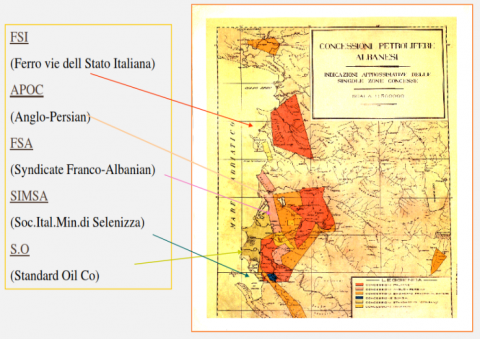
Until the year 1925, the Albanian government had granted petroleum exploration to several international oil companies: APOC (Anglo-Persian Oil Company); FSI (Ferrovie dello Stato Italiano); FSA (Syndicate Franco-Albanie); AIPA; SIMSA (Soc. Ital. Min. di Selenizza); S. O. (Standart Oil Company), as shown in Figure 1.
Figure 1. Oil fields and oil companies working in Albania, in 1925
A period of intensive exploration research started after the 1950s, resulting in discoveries of some important oilfields; Marinza, 1957; Visoka, 1963; Gorisht, 1966; Ballsh-Hekal, 1966; Finiq-Krane, 1973; Cakran-Mollaj, 1977; Amonica, 1980; Delvina, 1989; Marinza, 1957); and gas fields such as Divjaka,1963; followed by Frakulla, 1966; Panaja, 1987; Ballaj-Kryevidhi, 1983; Povelce 1987; Durres, 1988.
As a result, the oil and gas production of Albania grew rapidly, reaching a maximum production of 2,250,000 tons/year (or 6,165 tons/day, equal to 38,408 bbl/day, barrels/day) in 1974. The maximum amount of gas produced reached 940,000,000 Nm3/year (or 2,575,342 Nm3/day) in 1982 [21].
After reaching peak oil, production began to decline rapidly due to the decreased reservoir pressure in old oilfields, the aging of production technology, exploration failures, and economic and political factors. In the first half of the 1990s, oil production had a drastic decrease, reaching a minimum of 300,000 tons in the year 2000. After the 1990s, the new Albanian government declared the opening of the first licensing round for the onshore and offshore blocks. In 1995, the Albanian state offered a total area of 22,400 km2 divided into eight new blocks [22].
The other remaining blocks are operated by Albpetrol (Albanian National Oil Company) or by other oil and gas companies in collaboration with Albpetrol. Seismic research was conducted in the offshore and onshore blocks; 11,124 km of 2D seismic profiles and 1,400 km of 3D seismic profiles were acquired in the offshore blocks, and 1,800 km of 2D was conducted in the onshore blocks. In addition, six exploration wells were drilled in the blocks with total footage of 21,629 m, and six exploration wells were drilled in the onshore blocks, as shown in Figure 2.
Figure 2. Onshore and offshore exploration blocks and oil companies working in Albania
Because of this intensive research and investment, certain prospective formations have been concluded for gas and oil exploration.
Curve-fitting model is an effective technique that is frequently implemented in the historical production of fossil fuels [23].
Curve-fitting is best applied to geologically homogeneous areas that have a relatively unrestricted exploration history (not being closed or interrupted exploration for legal or political reasons). The well-known growth function is the best curve-fitting model to describe the production of limited and nonrenewed resources such as oil and gas production, minerals, etc.
The goodness-of-fit is often used to describe how well the model fits the historical data, as shown in Table 1. Similar, new or improved curves have been studied and turned out to be useful and effective for both descriptive and predictive purposes in the subject of oil and gas production [24, 25].
Generally, all forms of application of curve-fitting models can be described in three main steps:
Step 1: Choose a suitable mathematical function that can be fit the data set;
Step 2: Perform curve-fitting and introduce constraints to improve fit quality;
Step 3: Extrapolate the fitted model to project future production trends.
Free and reliable, correct public data are important to have a complete and correct analysis of the production history of a place, region, or country.
The data implemented in this article have been collected from several sites of state institutions [26, 27]. The data reflect the annual production of oil in Albania in the years 1929-2019, as shown in Table 2.
Table 1. Growth function to describe the production data
|
Model |
Equation of q(t) or Q(t) |
Parameters |
Inflection Point |
|
Hubbert |
$q(t)=U R R \frac{k \cdot \exp (-k(t-t m))}{[(1+\exp (-k(t-t m)))]^2}$ |
$t_m, k$ |
0.5 |
|
Gaussian |
$q(t)=U R R \frac{1}{s \sqrt{2 \pi}} \cdot\left[-\frac{(t-t m)^2}{2 s^2}\right]$ |
$s, t_m$ |
0.5 |
|
Weillbull |
$q(t)=U R R \frac{b+1}{c} \cdot t^b * \exp \left(-\frac{t^{b+1}}{c}\right)$ |
b, c |
$e^{-1}=0.37$ |
|
Rayleigh |
$q(t)=U R R \frac{1}{c^2} \cdot t * \exp \left(-\frac{t^2}{2 c^2}\right)$ |
c |
n. a |
|
HCZ |
$q(t)=U R R * a * \exp \left(-\frac{a}{b} \cdot e^{-b t}-b t\right)$ |
a, b |
$e^{-1}=0.37$ |
|
Gen. Weng |
$q(t)=U R R \frac{b+1}{c} \cdot t^b * \exp \left(-\frac{t^{b+1}}{c}\right)$ |
b, c |
<0.5 |
|
Gen. Verhulst |
$q(t)=U R R \frac{k}{n} \cdot \frac{\left(2^n-1\right) \exp \left(k\left(t-t_{0.5}\right)\right)}{\left[1+\left(2^n-1\right) \exp \left(k\left(t-t_{0.5}\,\right)\right)\right]^{\quad\frac{n-1}{n}}}$ |
$n, k, t_{0.5}$ |
n. a |
|
Exponential |
$q(t)=U R R * k * \exp (k(t-t m))$ |
$t_m, k$ |
n. a |
|
Logistic |
$Q(t)=U R R *(1+\exp (-k(t-t m)))^{-1}$ |
$t_m, k$ |
0.5 |
|
Gompertz |
$Q(t)=U R R * \exp (-\exp (-k(t-t m)))$ |
$t_m, k$ |
$e^{-1}=0.37$ |
|
Richards |
$Q(t)=U R R *(1+b * \exp (-k(t-t m)))^{-\frac{1}{b}}$ |
$t_m, b, k$ |
$(b+1)^{-\frac{1}{b}}$ |
Table 2. Oil production in Albania, 1929-2019
|
x 1000 |
|
x 1000 |
|
x 1000 |
|
x 1000 |
|
|
Year |
Ton |
Year |
Ton |
Year |
Ton |
Year |
Ton |
|
1929 |
0.8 |
1952 |
134 |
1975 |
1635 |
1998 |
340 |
|
1930 |
2.2 |
1953 |
130 |
1976 |
1508 |
1999 |
337 |
|
1931 |
4 |
1954 |
210 |
1977 |
1455 |
2000 |
330 |
|
1932 |
5 |
1955 |
232 |
1978 |
1392 |
2001 |
390 |
|
1933 |
8 |
1956 |
270 |
1979 |
1360 |
2002 |
412 |
|
1934 |
14 |
1957 |
485 |
1980 |
1276 |
2003 |
485 |
|
1935 |
35 |
1958 |
411 |
1981 |
1213 |
2004 |
464 |
|
1936 |
75 |
1959 |
643 |
1982 |
1276 |
2005 |
445 |
|
1937 |
105 |
1960 |
770 |
1983 |
1181 |
2006 |
518 |
|
1938 |
120 |
1961 |
790 |
1984 |
1223 |
2007 |
564 |
|
1939 |
137 |
1962 |
810 |
1985 |
1191 |
2008 |
578 |
|
1940 |
145 |
1963 |
780 |
1986 |
1181 |
2009 |
577 |
|
1941 |
152 |
1964 |
780 |
1987 |
1149 |
2010 |
742 |
|
1942 |
155 |
1965 |
880 |
1988 |
1033 |
2011 |
895 |
|
1943 |
126 |
1966 |
980 |
1989 |
801 |
2012 |
1028 |
|
1944 |
40 |
1967 |
1149 |
1990 |
654 |
2013 |
1205 |
|
1945 |
50 |
1968 |
1270 |
1991 |
601 |
2014 |
1368 |
|
1946 |
59 |
1969 |
1450 |
1992 |
622 |
2015 |
1279 |
|
1947 |
73 |
1970 |
1561 |
1993 |
516 |
2016 |
1056 |
|
1948 |
116 |
1971 |
1820 |
1994 |
506 |
2017 |
956 |
|
1949 |
137 |
1972 |
1980 |
1995 |
432 |
2018 |
910 |
|
1950 |
147 |
1973 |
2150 |
1996 |
380 |
2019 |
1025 |
|
1951 |
126 |
1974 |
2250 |
1997 |
350 |
|
|
3.1 The Hubbert model
Hubbert forecasted the future US oil production by fitting a curve to historical data on annual US production and projecting this forward in time under the assumptions that:
In his first presentation, in 1949, Hubbert did not produce a formula. In 1956, he produced the logistic formula for his bell curve model as shown in Figure 3.
Figure 3. Hubbert’s bell curve forecasting a peak in US oil production between 1965 and 1970
The key features of Hubbert’s logistic model are:
Cumulative production is modelled by a logistic function. Yearly production is modelled as the first derivative of the logistic function.
The production profile is symmetric (i.e., maximum production occurs when the resource is half-depleted and its functional form is symmetric on both sides of the curve).
Production increases and decreases in a single cycle without multiple peaks.
For any production curve of a finite resource, the production rate must begin at zero, and then after passing through one or several maxima, it must decline again to zero.
The area under the production rate curve (above the time axis), between the start time and the end time, is the URR amount (equivalent to EUR-Estimated Ultimate Recovery) [28].
Hubbert’s model of oil production is defined mathematically as follows:
$Q(t)=\frac{Q_{\infty}}{1+e^{-a(t-t m)}}\qquad, \quad q(t)=\frac{d Q(t)}{d t}=\frac{a Q_{\infty} \cdot e^{-a(t-t m)}}{\left(1+e^{-a(t-t m)}\quad\,\right)^2}$ (1)
where,
Q(t)-Cumulative production (tons, barrels- bbl),
q(t)-Production rate (tons/year, barrels- bbl/year),
$Q_{\infty}$-URR (Ultimate Recovery Reserves) (tons, barrels-bbl),
a- a coefficient that defines the “steepness” of the cumulative production curve,
$t m$-The time when cumulative production reaches one-half of the $Q_{\infty}$=URR, (year).
The multi-cycle model, introduced by Laherrere has been proven to fit the oil production data of several regions. In practice, the additional cycles can also result from efficient improvements in exploration and production methods, which can increase oil production significantly [29, 30].
The multi-cycle model is:
$Q(t)=\sum_{i=1}^k Q(t)_i=\sum_{i=1}^k\left\{\frac{2 Q_{\max }}{1+\cosh (b(t-t m))}\quad\right\}i$ (2)
where,
k-Total number of logistic curves that fit the production data;
Qmax- peak production rate (tons, barrels) and;
tm- Peak production time, respectively for each cycle (year).
3.2 The Gompertz model
The Gompertz function is another useful model that can successfully fit the world’s oil production from the year 2009 onward, resulting in an asymmetrical production profile [31]. It was developed by Gompertz in 1825, as a modification of the symmetric logistic function to an asymmetrical growth curve.
Gompertz and Logistic models generate very similar curves. But when Y is low, the Gompertz model grows more quickly than the logistic model. Conversely, when Y is large, the Gompertz model grows more slowly than the Logistic model. The cumulative and production rate functions are:
$Q(t)=P_{\max } \cdot e^{-e^{-k(t-T p)}}$ (3)
$q(t)=\frac{d Q}{d t}=P_{\max } \cdot k \cdot e^{-k\left(t-T_p\right)} \cdot e^{-e^{-k(t-T p)}}$ (4)
where,
Q(t)- cumulative oil production, (tons, barrels- bbl);
q(t)- production rate, (tons/year, barrels- bbl/year);
Pmax- maximum production rate, (tons/year, barrels- bbl/year);
Tp-year of peak production rate (year).
3.3 The Gaussian model
Another mathematical model, which may fit best in several cases, is the normal distribution, or the Gaussian model, because of its similar curve shape compared to Hubbert’s logistic model [32].
The Gaussian model works best with numerous independent wells and few regulatory constraints. The central limit theorem (CLT) is the justification for applying the Gaussian curve in statistical applications, as in this case. Based on oil production data in the US, it is concluded that over 20,000 oil producers in the USA are acting at random, "leading to a Gaussian curve", and the normal distribution model is the best-fit model [33].
The probability density function for a normal distribution is given by the formula:
$p(x)=\frac{1}{\sigma \sqrt{2 \pi}} \cdot e^{-\frac{(x-\mu)^2}{2 \sigma^2}},-\infty<x<\infty$ (5)
where,
μ- the mean, (the peak oil of the bell curve, time- year);
σ- the standard deviation (a parameter of the width of the bell curve);
If the three oil production rate parameters $Q_{\infty}, t_m, s$, are included in the original mathematical formula (5) then an adaptive Gaussian symmetrical model is produced:
$q(t)=\frac{Q_{\infty}}{s \sqrt{2 \pi}} \cdot e^{-\frac{\left(t-t_m\right)\,^2}{2 s^2}}$ (6)
where,
$Q_{\infty}$- the Ultimate Oil Recovery, (tons, barrels- bbl);
tm- time, year, at the maximum production rate, (time- year);
s- the width parameter of the bell curve.
The asymmetric model based on a Gaussian curve is given by the formula:
$q(t)=s_{d e c}-\frac{s_{d e c}-s_{i n c}}{1+e^{k\left(t-t_m\right)}}$ (7)
$Q(t)=q_{\max } \cdot e^{-\frac{\left(t-t_m\right)^2}{2(q(t))^2}}$ (8)
where,
Q(t)- the cumulative production rate in the year t, (tons/year, barrels- bbl/year);
$q_{\max }$- maximum production rate, (tons, barrels- bbl);
tm- time of peak oil production rate, - (year);
q(t)- the sigmoid function that changes the standard deviation near t=tm;
sinc- the standard deviation of the pre-peak production curve;
sdec- the standard deviation of the post-peak production curve.
3.4 DCA (Decline Curve Analyses) models
DCA is another method of predicting the future of oil and gas production rates. It is used to describe and analyse declining production rates and predict the future performance of oilfield production [34].
The production rate of oil and gas decreases over time, for several reasons, mainly due to the loss of reservoir pressure as well as the decrease in the amount of oil in the reservoir.
The DCA method is based on fitting a line to performance history and assuming that the same trend will continue going forward.
3.4.1 Exponential decline
The exponential decline represents the case when the production rate declines by the same percentage each period.
The equation is:
$q=q_0(1-d)^t$ (9)
where,
q=production rate at the time t;
qo=initial producing rate at the time to;
d=decline rate per period, (year, month);
t=time at which the calculation of q is required;
The cumulative production to a future time t is:
$Q(t)=\frac{q o\left(1-(1-d)^t\right)}{-\ln (1-d)}$ (10)
3.4.2 Hyperbolic decline
Production rates and cumulative functions are:
$q(t)=\frac{q_0}{(1+b d t)^{\frac{1}{b}}}$ (11)
$Q(t)=\frac{q_o{ }^b}{d \cdot(1-b)}\left[q_0{ }^{1-b}-q^{1-b}\right]$ (12)
where,
q=production rate at time t;
qo=initial production rate;
b=factor;
d=initial hyperbolic decline rate;
t=time;
3.4.3 Harmonic decline
When b=1, the equations will show the harmonic decline function. Production rate and cumulative functions are:
$q(t)=\frac{q_0}{1+d . t}$ (13)
$Q(t)=\frac{q_o}{d} * \ln (1+d t)$ (14)
The accumulation of petroleum in Albanian oilfields is related to two natural reservoirs: 75% of Petroleum reserves are contained in sandstone reservoirs and 25% in carbonate reservoirs. Oil is generally heavy, with a density of 30–380 API, and the depth of the oil and gas wells varies from 400–3,500 m [35].
The Albanian oil production data for the period 1919- 2019 are provided by the Albpetrol (National State Oil Company), AKBN (National Agency of Natural Resources), and Albgaz (National Gas Company).
Albanian oil production started in 1918, but there are no official data for the period 1918 to 1929.
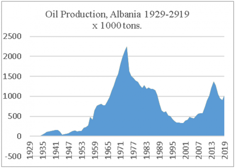
Albanian oil reached its peak oil in 1974 with a maximum production of 2,250,000 tons, equal to 1.4 Mbbl (million barrels) as shown in Table 3.
The curve produced from the past production data shows an asymmetric form, that can be explained by the influence of external factors (beyond geological, production performance, or other internal factors), which were political, social, and economic.
The sigmoid growth functions are considered the best models to present historical oil production data, such as Logistic, Ratkowsky, Gompertz, etc.
The production of oil from a single well, oilfield, region, or country, presents the same similar characteristics, the production at first increases exponentially, continues with a slower growth until it reaches peak production, and then the production declines until the resource is depleted in Figure 4, while cumulative oil production is shown in Figure 5.
Figure 4. Albanian oil production (ktons/ year), 1929- 2019
Figure 5. Cumulative oil production (ktons), 1929-2019
Table 3. Albania oil production 1929-2019
|
Start |
1929 |
|
Peak oil year |
1974 |
|
Peak oil production (tons) |
2,250,000 |
|
Peak oil production (barrels- bbl) |
14,377,500 |
|
Peak oil cumulative production, until 1974 (tons) |
47,708,800 |
|
Peak oil cumulative production, until 1974 (barrels- bbl) |
304,859,232 |
|
Total cumulative production 1929-2000 (tons) |
62,605,800 |
|
Total cumulative production 1929-2000 (barrels- bbl) |
400,051,062 |
|
Peak oil cumulative production/ total |
76% |
|
Total Albanian oil reserves (tons) |
430,000,000 |
|
Total recoverable reserves (tons) |
82,000,000 |
|
Remaining recoverable reserves (tons) |
19,394,200 |
The most suitable curves for production data were found to be the asymmetric ones, such as Gaussian, Logistic, Exponential, etc. Continuing with the production curve asymmetry, the average ratio for the increasing curve was 12% and for the declining curve was 8%, meaning the production increase rate was much faster than the decreasing rate.
Brandt [36] described the asymmetrical exponential model as the best fit for Albanian historical production data as shown in Figure 6. The Gaussian model is also applied to the oil production rate data as shown in Figure 7. Logistic and Gaussian curves are generated also for the cumulative production data as shown in Figures 8 and 9. Three parameters are calculated for each model, as shown in Table 4.
Most of Albania's oil fields are still active and producing, albeit at a decreasing rate. Until the peak year, around 23 Mtons were produced from all the oilfields.
Until the year 2000, the total oil production was 47 Mtons, and until the year 2019, the cumulative oil production was 62 Mtons (400 Mbbl). The reserve estimation for Albania is around 400 Mtons, and the recoverable reserves are around 80 Mtons, meaning that 20 Mtons remain to be extracted. With the advancements in technology and exploitation methods, the number of remaining reserves may be higher [37].
Figure 6. Asymmetric exponential fit, Albania production [15]
Figure 7. Gaussian fit for Albanian oil production data 1929- 2019
Figure 8. The logistic fit (Hubbert curve)
Figure 9. The Gaussian fit
Table 4. The models and parameters
|
Gaussian Model: |
|
Equation: a*exp (-(x-b)2/(2*c2)) a=4.67E+04 b=1.99E+03 c=1.75E+01 Correlation Coefficient: 9.988E-01 |
|
Logistic Power: |
|
Equation: a/(1+(x/b)**c) a=4.87E+04 b=1.97E+03 c=-2.77E+02 Correlation Coefficient: 9.997E-01 |
This study was designed to scrutinize historical oil production data and identify the most suitable model for data representation and future production prediction. The Hubbert model is commonly regarded as one of the most dependable models for describing historical production data and predicting future data for finite resources, including oil and gas, minerals, and more.
Hubbert's symmetric monocyclic model exhibits high reliability when applied to a natural field that remains unaffected by external factors, and to regions comprising multiple independent oil fields. Under optimal conditions, the oil production curve manifests symmetry, where the descent curve mirrors the ascent curve, and upon reaching peak oil, half of the reserve is depleted. However, this symmetrical pattern is not typically observed.
Successful curve fitting is generally achieved when the production data series has exceeded the inflection point and peak oil, and when there exists a singular production cycle, thereby establishing the most dependable model. Less reliable models are derived when the production data series has surpassed the inflection point but not peak oil. In instances where neither point is achieved, creating a reliable model to depict the production cycle becomes exceedingly challenging.
During the production decline phase, where oilfield production is decelerating, decline curve analyses (DCA) can be utilized to forecast future production.
Historical production data from Albania generates a monocyclic and asymmetric curve. The zenith of Albanian oil production was in 1974, accounting for nearly 70% of total recoverable reserves. The average increasing ratio of Albanian oil production is 12%, and the average decreasing ratio is 9%, thus highlighting the asymmetrical nature of the oil production curve.
Estimating oil reserves and possessing comprehensive knowledge of a well-documented resource's production history can furnish a model for assessing the reserves and production of lesser-known or newly discovered resources. This is attained through the amalgamation of other methods such as the analogy method and by considering and comparing similar geological parameters for both locales.
The scope of this article is confined to the analysis of national oil and gas production in Albania, for which complete data was successfully procured. For an enhanced comprehension of the oil and gas production scenario in Albania, it would be beneficial to obtain comprehensive data on well-established oilfields with a history spanning over 60 years of oil and gas production.
[1] Nashawi, I.S., Malallah, A., Al-Bisharah, M. (2010). Forecasting world crude oil production using multicyclic Hubbert model. Energy & Fuels, 24(3): 1788-1800. https://doi.org/ 10.1021/ef901240p.
[2] Sorrell, S., Speirs, J. (2014). Using growth curves to forecast regional resource recovery: Approaches, analytics and consistency tests. Philosophical Transactions of the Royal Society A: Mathematical, Physical and Engineering Sciences, 372(2006): 20120317. https://doi.org/10.1098/rsta.2012.0317
[3] Laherrere, J.H. (1999). World oil supply- what goes up must come down, but when will it peak? Oil and Gas Journal, 97(5): 57-64.
[4] Campbell, C.J., Laherrere, J.H. (1998). Preventing the next oil crunch—The end of cheap oil. Scientific American, 3: 78-83. http://www-personal.umich.edu/~twod/oil/NEW_SCHOOL_COURSE2005/articles/research-oil/campbell_laherrere_sci_am_mar1998.pdf.
[5] Bentley, R.W. (2002). Global oil & gas depletion: An overview. Energy Policy, 30(3): 189-205. https://doi.org/10.1016/S0301-4215(01)00144-6
[6] Hubbert, M.K. (1975). Hubbert Estimates from 1956 to 1974 of US Oil and Gas. Grenon, M.(ed.). Methods and Models for Assessing Energy Resources. https://doi.org/10.1016/B978-0-08-024443-3.50038-8
[7] Wood, J.H., Long, G.R., Morehouse, D.F. (2003). World conventional oil supply expected to peak in 21st century. Offshore (Conroe, Tex.), 63(4): 90-94.
[8] Hallock, J.L., Tharakan, P.J., Hall, C.A., Jefferson, M., Wu, W. (2004). Forecasting the limits to the availability and diversity of global conventional oil supply. Energy, 29(11): 1673-1696. https://doi.org/10.1016/j.energy.2004.04.043
[9] Brandt, A.R. (2007). Testing Hubbert. Energy Policy, 35(5): 3074-3088. https://doi.org/10.1016/j.enpol.2006.11.004
[10] Xu, D., Zhu, Y. (2020). A copula–Hubbert model for co (by)-product minerals. Natural Resources Research, 29(5): 3069-3078. https://doi.org/10.1007/s11053-020-09643-1
[11] Maggio, G., Cacciola, G. (2009). A variant of the Hubbert curve for world oil production forecasts. Energy Policy, 37(11): 4761-4770. https://doi.org/10.1016/j.enpol.2009.06.053
[12] Maggio, G., Cacciola, G. (2012). When will oil, natural gas, and coal peak? Fuel, 98: 111-123. https://doi.org/10.1016/j.fuel.2012.03.021
[13] Ebrahimi, M., Ghasabani, N.C. (2015). Forecasting OPEC crude oil production using a variant Multicyclic Hubbert Model. Journal of Petroleum Science and Engineering, 133: 818-823. https://doi.org/10.1016/j.petrol.2015.04.010
[14] Brandt, A.R. (2007). Testing Hubbert. Energy Policy, 35(5): 3074-3088. https://doi.org/10.1016/j.enpol.2006.11.004
[15] Saraiva, T.A., Szklo, A., Lucena, A.F.P., Chavez-Rodriguez, M.F. (2014). Forecasting Brazil’s crude oil production using a multi-Hubbert model variant. Fuel, 115: 24-31. https://doi.org/10.1016/j.fuel.2013.07.006
[16] Métois, M., Benjelloun, M., Lasserre, C., Grandin, R., Barrier, L., Dushi, E., Koçi, R. (2020). Subsidence associated with oil extraction, measured from time series analysis of Sentinel-1 data: case study of the Patos-Marinza oil field, Albania. Solid Earth, 11(2): 363-378. https://doi.org/10.5194/se-11-363-2020
[17] Cani, X., Malollari, I., Beqiraj, I., Manaj, H., Premti, D., Lorina, L.İ.Ç.İ. (2016). Characterization of crude oil from various oilfields in Albania through the instrumental analysis. Journal of International Environmental Application and Science, 11(2): 223-228. https://dergipark.org.tr/tr/download/article-file/571600
[18] Ndreko, D., Nazaj, S. (2020). Tectonic model of the Kreshpan-verbas region and oil reservoir related with it. International Symposium for Environmental Science and Engineering Research. https://iseser.com/year/2020/paper/19/.
[19] Kosova, R., Xhafaj, E., Karriqi, A., Boci, B., Guxholli, D. (2022). Missing data in the oil industry and methods of imputations using Spss: The Impact on reserve estimation. Journal of Multidisciplinary Engineering Science and Technology, 9(2): 15146-15155. https://www.jmest.org/wp-content/uploads/JMESTN42354004.pdf.
[20] https://albpetrol.al/marreveshjet-hidrokarbure-3/, accessed on 22nd December 2022.
[21] https://albgaz.al/historiku-i-gazit/, accessed on 22nd December 2022.
[22] http://www.gsa.gov.al/, accessed on 22nd December 2022.
[23] Wang, J., Feng, L. (2016). Curve-fitting models for fossil fuel production forecasting: Key influence factors. Journal of Natural Gas Science and Engineering, 32: 138-149. https://doi.org/10.1016/j.jngse.2016.04.013
[24] Anderson, K.B., Conder, J.A. (2011). Discussion of multicyclic Hubbert modelling as a method for forecasting future petroleum production. Energy & Fuels, 25(4): 1578-1584. https://doi.org/10.1021/ef1012648
[25] Höök, M., Li, J., Oba, N., Snowden, S. (2011). Descriptive and predictive growth curves in energy system analysis. Natural Resources Research, 20: 103-116. https://doi.org/10.1007/s11053-011-9139-z
[26] https://albpetrol.al/prodhimi-i-naftes-nder-vite/, accessed on 22nd December 2022.
[27] http://www.akbn.gov.al/wp-content/uploads/2013/, accessed on 22nd December 2022.
[28] Hubbert, M.K. (1949). Energy from fossil fuels. Science, 109(2823): 103-109. https://doi.org/10.1126/science.109.2823.103
[29] Campbell, C.J. (2013). The oil age in perspective. Energy Exploration & Exploitation, 31(2). https://doi.org/10.1260/0144-5987.31.2.149
[30] Sorrell, S., Speirs, J. (2010). Hubbert’s legacy: A review of curve-fitting methods to estimate ultimately recoverable resources. Natural Resources Research, 19: 209-230. https://doi.org/10.1007/s11053-010-9123-z
[31] Carlson, W.B. (2010). The modelling of world oil production using sigmoidal functions-Update 2010. Energy Sources, Part B: Economics, Planning, and Policy, 6(2): 178-186. https://doi.org/10.1080/15567249.2010.516310
[32] Bartlett, A.A. (2000). An analysis of U.S. and world oil production patterns using Hubbert-style curves. Mathematical Geology, 32: 1-7. https://doi.org/10.1023/A:1007587132700
[33] Peebles, T., Ague, J., Oristaglio, M. (2017). Development of Hubbert’s peak oil theory and analysis of its continued validity for us crude oil production. Department of Geology and Geophysics, Yale University. https://earth.yale.edu/sites/default/files/files/Peebles_Senior_Essay.pdf.
[34] Kosova, R., Muça, M., Sinaj, V. (2013). Decline curve analyses and oil production forecast. International Journal of Science and Research (IJSR), 4(10): 864-866.
[35] Prifti, I., Muska, K. (2013). Hydrocarbon occurrences and petroleum geochemistry of Albanian oils. Italian Journal of Geosciences, 132(2): 228-235. https://doi.org/10.3301/IJG.2012.29
[36] Brandt, A.R. (2010). Review of mathematical models of future oil supply: Historical overview and synthesizing critique. Energy, 35(9): 3958-3974. https://doi.org/10.1016/j.energy.2010.04.045
[37] Kosova, R., Shehu, V., Naco, A., Xhafaj, E., Stana, A., Ymeri, A. (2015). Monte Carlo simulation for estimating geologic oil reserves. A case study from Kucova Oilfield in Albania. Muzeul Olteniei Craiova. Oltenia. Studii şi comunicări. Ştiinţele Naturii, 31(2): 20-25. https://biozoojournals.ro/oscsn/cont/31_2/Cover_Content_31-2.pdf.