Abdul-Sattar J. Al-Saif | Takia Ahmed J. Al-Griffi*
© 2020 IIETA. This article is published by IIETA and is licensed under the CC BY 4.0 license (http://creativecommons.org/licenses/by/4.0/).
OPEN ACCESS
In this research, we have proposed a new technique to solve two-dimensional (2D) viscous fluid flow among slowly expanding or contracting walls. The new technique depends on combining the algorithms of Yang transform and the homotopy perturbation methods. The results, obtained from the first iteration and by using the new method, show the accuracy and efficiency of this method compared to the other methods, used to find the analytical approximate solution for the problem caused by the 2D viscous fluid flow. Moreover, the graphs of the new solutions show the validity, usefulness and necessity of the new method.
Yang transform, homotopy perturbation method, 2D viscous flow, convergence analysis
One of the most common problems of the fluid flow and which has interested many researchers is the laminar flow of viscous fluid through a porous channel or pipe with contracting or expanding permeable walls. This great interest is due to its biological applications, like the conveyance of biological fluids through expanding or contracting receptacles, nomination in the lungs and kidneys, flow inside the lymphatic's, and many others besides. Many scientists and researchers have attempted to find solutions for these equations using different methods; for example, the first scientists who found a solution to the two-dimensional laminar flow of a viscous fluid problem in a parallel-walled channel is Berman [1]. He found the solution to this problem by using the perturbation method. He utilized the Reynolds number as a perturbation parameter, where the solution is valid for small values of the Reynolds number. Ganji et al. [2] applied the homotopy perturbation method (HPM) to solve 2D viscous fluid flow problem between slowly expanding or contracting walls. Comparing their results with the numerical method (NM), they noted that HPM is efficacious and simple and can be used to solve nonlinear problems. Moreover, their results demonstrate that HPM is capable to solve this problem with quickly convergence approximations without any restrictive supposition or transformations, which lead to changes in the physical definition of the problem. Dinarvand [3] found a solution for the viscous fluid flow through slowly expanding or contracting walls by using the differential transform method. He compared between his results and the ones obtained from the numerical method to find that his results exhibit the marked accuracy. Moreover, from these results, he noticed that the differential transform method does not demand small parameters in the equations, therefor, this method can be applied to many nonlinear differential and integral equations without perturbation, linearization, or discretization. Dinarvand et al. [4] used the homotopy analysis method (HAM) to find the solutions for the viscous fluid flow with expanding or contracting gaps. They compared the obtained results with the numerical method and the results demonstrate a remarkable accuracy. This method (HAM) differs from perturbation methods in that it does not rely on small parameters. So, it is valid for both mighty and weak nonlinear problems. Sushila et al. [5] used the Sumudu transform homotopy perturbation method (HPSTM) to solve the problem of the viscous fluid flowing between slowly expanding or contracting walls. Numerical results have shown that these methods are very effective and able to solve this problem. Moreover, they observed that this method was able to find the solution without any restrictive suppositions to the rise of changes in the physical definition of the problem. They also noted that the advantage of this method is that it solves nonlinear problems without utilizing Adomian’s polynomials. Ledari et al. [6] solved the viscous fluid flow problem by slowly expanding or contracting walls by using Akbari Ganji’s Method (AGM). They compared the results of AGM with those of the Ruge-Kutta method, the Adomian decomposition method, the homotopy perturbation method and variational iteration method; the results show that this method is efficacious and has enough accuracy.
Despite all these advantages of the methods, used by researchers to solve the current problem (as illustrated in available literature), there are some disadvantages to these methods, for example, some of these methods require high iterations to obtain an accurate solution to the current problem. Also, some of these methods require a great deal of time and effort to solve the problem.
There are many analytical methods, some of which need a perturbation parameter and others do not need one. One of these methods that do not need perturbation parameters is the Yang transform method (YT), which is a new integral transform proposed in 2016 by Yang [7]. It was first applied to the heat transfer equation in the steady-state. Note that this method is precise and efficacious in finding the analytical solutions to linear differential equations (partial), and it is used by many researchers to solve different problems [7, 8]. In 2018, Dattu [9] illustrated the fundamental properties of YT and he utilized this method to solve differential equations with constant coefficients, and he also defined the Laplace-Yang dual property.
One of the analytical methods that depended on the small perturbation parameter is the new homotopy perturbation method, which is a new shape, derived from the homotopy perturbation method (HPM). It was discovered in 2010 by Aminikhah and Hemmatnezhad [10] while they were trying to find an analytical approximate solution to partial and ordinary differential equations. In this method, the solution is assumed to be an infinite series which converges readily to the exact solution. Many researchers used this method to solve various equations [11, 12] and they noted that it's a powerful, effective, easy and accurate tool to solve linear and nonlinear differential equations, compared to the standard homotopy perturbation method.
From the scientific research, conducted by researchers using these two methods (YT & HPM), it is found that they are powerful and effective for finding approximate analytical solutions to the non-linear and linear differential equations (partial/ordinary). Despite the above positive points, there are some negative points to these two methods (depending on the literature review above and to the best of our knowledge) such as, the HPM mostly requires high iterations to obtain an approximate analytical solution as well as the Yang's method may not succeed in finding the exact solution, especially to non-linear problems that are similar to the current problem.
All these reasons led us to suggest a new method to overcome these negatives points and reduce the number of iterations in finding analytical approximate solutions, and as well as saving time and effort spent in solving the nonlinear problem.
The main purpose of this paper is to introduce a newly developed method to solve the two- dimensional viscous fluid flow problem among slowly expanding or contracting walls. The new method is based on combining the Yang transform [7] and the new homotopy perturbation method [10] named the Yang transform-homotopy perturbation method (YTHPM). The numerical results, obtained by using the new method, prove that the efficiency, activity, and high accuracy of this method in comparison with other methods.
The basic ideas of YTHPM depend on the algorithms of YT and HPM, which will be discussed in this section.
2.1 Yang transform method
Integrative transformations such as the transformations of Laplace, Sumudu, and Elzaki and others, have wide applications in different fields of science and engineering like fluid mechanics, viscosity, physics, finance and chemistry [13] etc. Because many operations and phenomena of science, engineering and real-life can be expressed mathematically and solved by using integral transforms. The problems (fluid mechanics, viscosity, ...) arising in these fields can be readily treated with the assistance of integral transforms by converting them into a mathematical form. In the course of time, researchers have become more attentive to solving the problems of science, space, engineering by presenting new integral transforms. In 2016, Yang [7] proposed a new integral transform called Yang Transform that was first applied to the heat transfer equation in the steady-state. Note that this method is accurate and effective for finding analytical solutions to linear differential equations (partial or ordinary), which is defined by the function g(t) and denoted by Y{g(t)} or T(s) as follows:
Y{g(t)}=T(s)=∞∫0e−ts g(t)dt (1a)
If we substitute, x=ts then Eq. (1a) becomes
Y{g(t)}=T(s)=s∞∫0e−x g(sx)dx (1b)
The YT has many properties, among which are the ones listed below:
(i) Y(1)=s
(ii) Y(t)=s2
(iii) Y(tn)=n!sn+1.
(iv) Y(eσt)=s1−σs
(v) Y(sin(σt))=σs21+σ2s2
(vi) Y(cos(σt))=s1+σ2s2
(vii) Y(sinh(σt))=σs21−σ2s2
(viii) Y(cosh(σt))=s1−σ2s2
2.1.1 Essential notion of the Yang transform
To clarify the essential notion of the Yang transform, we meditate the linear equation in the differential operator form as follows:
L1(v)+R(v)=q (2a)
where, the linear terms L1(v)+R(v), and q are functions. If we assume that L1=∂∂t, and then take the Yang transforms for both sides of Equation (2a), we have: Y(L1(v)+R(v))=Y(q), from the derivative property of YT [9], we get: 1sY(v)−v(0)=Y(q−R(v)), the rearrangement of the above equation, yields:
Y(v)=s(Y{q−R(v)}+v(0)) (2b)
By taking the inverse Yang transform for both sides of Eq. (2b), we have the solution in the form:
v=Y−1[s(Y{q−R(v)}+v(0))] (2c)
An illustrative example of YT for differential equation appears as follows [9]:
Consider the 2nd order ordinary differential equation as:
y′′(t)+y(t)=0withy(0)=y′(0)=1 (2d)
By taking YT for both sides of Eq. (2d), we have: T(s)s2−y(0)s−y′(0)+T(s)=0, Then: T(s)=s21+s2+s1+s2. Taking YT inverse and from the property of YT, we get: y(t)=sin(t)+cos(t).
2.2 Homotopy perturbation method (HPM)
A new format of the homotopy perturbation method was discovered in (2010) by Aminikhah and Hemmatnezhad [10] in their attempt to solve ordinary and partial differential equations. They imposed the form of a solution that results from using this method as an infinite series. The researchers' use of this method proves that it is a powerful and effective method to find the solutions to nonlinear differential equations, compared to the standard homotopy method.
2.2.1 Fundamental idea of the HPM: [10, 11]
To clarify the fundamental idea of HPM, lets contemplate the general nonlinear equation in the differential operators forms as:
A1(v)−q(r)=0,r∈Ω1 (3)
Together with the conditions of the boundary:
B1(v,∂v∂n)=0,r∈Γ1 (4)
where, Β1 is the operator of the boundary; q(r) is the known function and Γ1 is the boundary of the domain Ω1; and A1 is a differential operator which can be divided into two parts: N1 nonlinear and L1 linear operator. So, Eq. (3) can be written as follows:
L1(v)+N1(v)−q(r)=0 (5)
By the technique of the homotopy, we build a homotopy u(r,β):Ω1×[0,1]→R, which achieves:
H1(u,β)=(1−β)[L(u)−v0)]+β[A1(u)−q(r)]=0,β∈[0,1] , r∈Ω1 (6)
Or
H1(u,β)=L1(u)−v0+β(v0)+β[N1(u)−q(r)]=0 (7)
where, β∈[0,1] is an embedding parameter, and v0 is an initial condition of Eq. (3). Clearly, from Eqns. (6) and (7), we have:
H1(u,0)=L1(u)−v0=0 (8)
H1(u,1)=L1(u)+N1(u)−q(r)=0 (9)
Suppose that the solutions of Eqns. (6) and (7) as a force chain in β as:
u=∞∑n=0βnun (10)
Now, we rewrite Eq. (7) in the form of:
L1(u)−v0+β[N1(u)−q(r)+v0]=0 (11)
By taking the L−11 of Eq. (11) to both sides, we get:
u=L−11(v0)+β[L−11(q(r))−L−11(N1(u))−L−11(v0)] (12)
Postulate that the initial approximation of Eq. (3) as follows:
v0=∞∑n=0an pn (13)
where, a0, a1, a2,… are the coefficients which are unknown and p0, p1, p2,… are special functions that rely on the problem. Through putting (10) and (13) into Eq. (12), we get:
∑∞n=0βnun=L−11(∑∞n=0anpn)+β[L−11(q(r))−L−11(N1(∑∞n=0βnun))−L−11(∑∞n=0anpn)] (14)
Comparing the coefficients which have the same powers of β leads to:
β0: u0=L−11(∞∑n=0anpn)β1: u1=L−11(q(r))−L−1(∞∑n=0anpn)−L−1(N1(u0))β2: u2=−L−11(N1(u0,u1))⋮βj: uj=−L−11(N1(u0,u1,...,uj−1))⋮ (15)
Now, if we assume that u1=0, then Eq. (15) results in u2= u3=...=0. Then, the exact solution can be found as follows:
v=u0=L−1(∞∑n=0anpn) (16)
2.3 Fundamental notion of YTHPM
Now, to demonstrate the fundamental notion of the new technique for Eq. (5) with the initial condition v(x, 0), firstly we apply the HPM property, then take the YT of both sides of the equation and apply its properties. Then, we take the inverse of the YT. Finally, we apply the HPM property to the function and conditions and find the solution, which can be summarized in the following steps:
Step 1: By the HPM, we have:
L1(u)−v0+β(v0)+β[N1(u)−q(r)]=0 (17)
Step 2: Taking the Yang transform for both sides of Eq. (17), we get:
Y(L1(u)−v0+β(v0)+β[N1(u)−q(r)])=0 (18)
Step 3: Postulate that L1=∂∂t, then by the differential property of Yang transform, we obtain:
1sY(u)−u(0)−Y(v0)+Y(β(v0))+Y(β[N1(u)−q(r)])=0 (19)
The rearrangement of Eq. (19), yields:
Y(u)=su(0)+sY(v0)−sY(β(v0))−sY(β[N1(u)−q(r)]) (20)
Step 4: Taking the Yang inverse for both sides of Eq. (20), we get:
u=Y−1(su(0))+Y−1(sY(v0))−Y−1(sY(β(v0))) −Y−1[sY(β[N1(u)−q(r)])] (21)
Step 5: Via the NHPM, we suppose that u=∑∞n=0βnun, v0=∑∞n=0anpn, u(0)=v(x,0), then, Eq. (21) becomes:
∞∑n=0βnun=Y−1(su(0))+Y−1{sY(∞∑n=0an pn)} −Y−1{sY[β(∞∑n=0an pn)]}−Y−1[sY(β[N1(∞∑n=0βnun)−q(r)])] (22)
Step 6: By equalizing the terms that have the same power of β, we have:
β0:u0=Y−1(su(0))+Y−1{sY(∑∞n=0anpn)}
β1:u1=−Y−1{sY(∑∞n=0anpn)}−Y−1[sY(N1(u0)−q(r))]
β2:u2=−Y−1[sY(N1(u0,u1))]⋮ (23)
Step 7: The analytical approximate solution can be found by putting β=1, v=limβ→1u=u0+u1+u2+⋯.
Consider laminar, incompressible and viscous fluid flow in a rectangular domain bounded by two permeable surfaces that allow to the viscous fluid to come in or way out through the consecutive expansions or contractions, as illustrated in Figure 1 [4].
Figure 1. The pattern of a rectangular domain with extended or contracted walls
Walls contract or expand orderly at a time-dependent rate a*(t). At the wall, the fluid flow velocity Uw is assumed to be independent of a locus. Beneath these presumptions, the continuity and motion equations are:
∂u⃛
\frac{\partial \dddot{u}}{\partial t}+\dddot{u} \frac{\partial \dddot{u}}{\partial \dddot{x}}+\dddot{v} \frac{\partial \dddot{u}}{\partial \dddot{y}}=\left(-\frac{1}{\rho}\right) \frac{\partial \dddot{P}}{\partial \dddot{x}}+v\left(\frac{\partial^{2} \dddot{u}}{\partial \dddot{x}^{2}}+\frac{\partial^{2} \dddot{u}}{\partial \dddot{y}^{2}}\right) (24a)
\frac{\partial \dddot{v}}{\partial t}+\dddot{u} \frac{\partial \dddot{v}}{\partial \dddot{x}}+\dddot{v} \frac{\partial \dddot{v}}{\partial \dddot{y}}=\left(-\frac{1}{\rho}\right) \frac{\partial \dddot{P}}{\partial \dddot{y}}+v\left(\frac{\partial^{2} \dddot{v}}{\partial \dddot{x}^{2}}+\frac{\partial^{2} \dddot{v}}{\partial \dddot{y}^{2}}\right) (24b)
where, \dddot{u}, \dddot{v} indicate the components for velocity in the \dddot{x}, \dddot{y} trends, t the time, ρ its density, \dddot{P} the pressure dimensional term, and v is the kinematic viscosity.
The boundary conditions are given as:
if \dddot{y}=a(t) then \dddot{u}=0, \quad \dddot{v}=-U_{w}=-\frac{a^{*}}{z}
if \dddot{y}=0 then \frac{\partial \dddot{u}}{\partial \dddot{y}}=0, \quad \dddot{v}=0
if \dddot{x}=0 then \dddot{u}=0 (25)
where, z=\frac{a^{*}}{U_{w}} is the permeance of the wall or the coefficient of suction/ injection, which is a gauge for wall permeability. The vorticity and stream functions can be presented by setting \dddot{u}=\frac{\partial \dddot{\psi}}{\partial \dddot{y}} and \dddot{v}=-\frac{\partial \dddot{\psi}}{\partial \dddot{x}}:
\dddot{\eta}=\dddot{v}_{\dddot{x}}-\dddot{u}_{\dddot{y}} (26a)
\frac{\partial \dddot{\eta}}{\partial t}+\dddot{u} \frac{\partial \dddot{\eta}}{\partial \dddot{x}}+\dddot{v} \frac{\partial \dddot{\eta}}{\partial \dddot{y}}=v\left(\frac{\partial^{2} \dddot{\eta}}{\partial \dddot{x}^{2}}+\frac{\partial^{2} \dddot{\eta}}{\partial \dddot{y}^{2}}\right) (26b)
By putting (26a) into (26b), we get:
\dddot{v}_{\dddot{x} t}-\dddot{u}_{\dddot{y} t}+\dddot{u}\left(\dddot{v}_{\dddot{x} \dddot{x}}-\dddot{u}_{\dddot{y} \dddot{x}}\right)+\dddot{v}\left(\dddot{v}_{\dddot{x} \dddot{y}}-\dddot{u}_{\dddot{y} \dddot{y}}\right)= \dddot{v}\left(\dddot{v}_{\dddot{x} \dddot{x} \dddot{x}}-\dddot{u}_{\dddot{y} \dddot{x} \dddot{x}}+\dddot{v}_{\dddot{x} \dddot{y} \dddot{y}}-\dddot{u}_{\dddot{y} \dddot{y} \dddot{y}}\right) (27)
Because of the mass conservation, an analogous solution can be advanced with respect to \dddot{x} [14]. Let:
\dddot{u}=\frac{v \dddot{x}}{a^{2}} \dddot{h}_{\zeta}, \quad \dddot{v}=-\frac{v}{a} \dddot{h}(\zeta, t), \quad \dddot{\Psi}=-\frac{v \dddot{x}}{a} \dddot{h}(\zeta, t) (28)
where, \dddot{h}_{\zeta}=\frac{\partial \dddot{h}(\zeta, t)}{\partial \zeta}, \quad \zeta=\frac{\dddot{y}}{a}.
From Eqns. (27) and (28), we possess:
\dddot{u}_{\dddot{y} t}+\dddot{u} \dddot{u}_{\dddot{y} \dddot{x}}+\dddot{v} \dddot{u}_{\dddot{y} \dddot{y}}=v\left(\dddot{u}_{\dddot{y} \dddot{x} \dddot{x}}+\dddot{u}_{\dddot{y} \dddot{y} \dddot{y}}\right) (29)
For solving Eq. (29), the chain rule is used to get:
\dddot{h}_{\zeta \zeta \zeta \zeta}+\alpha(t)\left(\zeta \dddot{h}_{\zeta \zeta \zeta}+3 \dddot{h}_{\zeta \zeta}\right) +\dddot{h} \dddot{h}_{\zeta \zeta \xi}-\dddot{h}_{\zeta} \dddot{h}_{\zeta \zeta}-\frac{a^{2}}{v} \dddot{h}_{\zeta \zeta t}=0 (30)
Together with the conditions of boundary:
when \zeta=0 then \dddot{h}=0, \dddot{h}_{\zeta \zeta}=0 (31a)
when \zeta=1 then \dddot{h}=\operatorname{Re}, \dddot{h}_{\zeta}=0 (31b)
where, \alpha(t)=\frac{a a^{*}(t)}{v} is the dimensionless dilation rate of the wall, which is negative for contraction and positive for expansion. R e=\frac{a U_{w}}{v} is the Reynolds number, which is negative for suction and positive for injection.
If the dimensionless set is defined, Eqns. (28, 30, 31) can be normalized as follows: u=\frac{\dddot{u}}{a^{*}}, v=\frac{\dddot{v}}{a^{*}}, \Psi=\frac{\dddot{\psi}}{a a^{*}}, x=\frac{\dddot{x}}{a}, h=\frac{\dddot{h}}{R e}, then: u=\frac{x h^{\prime}}{z}, v=\frac{-h}{z}, \Psi=\frac{x h}{z}, z=\frac{\alpha}{R e}.
Thus, Eq. (30) becomes:
\begin{align} & {{h}_{\zeta \zeta \zeta \zeta }}+\alpha \,(\zeta \ {{h}_{\zeta \zeta \zeta }}+3{{h}_{\zeta \zeta }}) \\ & +\operatorname{Re}h\,{{h}_{\zeta \zeta \zeta }}-\operatorname{Re}{{h}_{\zeta }}{{h}_{\zeta \zeta }}=0 \\ \end{align} (32)
And boundary conditions are:
h=0,\ {{h}_{\zeta \zeta }}=0 when \zeta =0 \\ And \,\,\, h=1,\ {{h}_{\zeta }}=0 when \zeta =1 (33)
If α=0 in Eq. (32), then Berman’s model [1] is obtained.
Now, we apply the algorithm of YTHPM for Eq. (32) with the boundary condition (33). The basic steps of the new technique are illustrated as follows:
Step 1: By HPM, we obtain:
{{h}_{\zeta \zeta \zeta \zeta }}-h_{0}^{*}+\beta \,h_{0}^{*}+\beta \,\left( \alpha (\zeta \,{{h}_{\zeta \zeta \zeta }}+3{{h}_{\zeta \zeta }})+\operatorname{Re}\,h\,{{h}_{\zeta \zeta \zeta }}-\operatorname{Re}\,{{h}_{\zeta }}\,{{h}_{\zeta \zeta }} \right)=0; h_{0}^{*}=\sum\limits_{i=0}^{\infty }{{{a}_{i}}{{\zeta }^{i}}}
Step 2: Taking the Yang transform for both sides of the equation in step (1), we have:
\begin{align} & \frac{1}{{{s}^{4}}}\tilde{h}-\frac{1}{{{s}^{3}}}h\,(0)-\frac{1}{{{s}^{2}}}h'(0)-\frac{1}{s}h''(0)-h'''(0)\,\,-Y(h_{0}^{*})+\beta \,Y(h_{0}^{*}) \\ & +\beta \,Y\,\left( \alpha \,(\zeta \,{{h}_{\zeta \zeta \zeta }}+3{{h}_{\zeta \zeta }})+\operatorname{Re}\,h\,{{h}_{\zeta \zeta \zeta }}-\operatorname{Re}\,{{h}_{\zeta }}\,{{h}_{\zeta \zeta }} \right)=0 \\ \end{align}
since h(0)=h^{\prime \prime}(0)=0 and h^{\prime}(0)=a, h^{\prime \prime \prime}(0)=b to be specified from the boundary conditions; by rearranging this equation, we get:
\begin{align} & \tilde{h}={{s}^{2}}a+{{s}^{4}}b+{{s}^{4}}Y(h_{0}^{*})-\beta \,{{s}^{4}}Y(h_{0}^{*}) \\ & \quad -\beta \,{{s}^{4}}Y\,\left( \alpha (\zeta \,{{h}_{\zeta \zeta \zeta }}+3{{h}_{\zeta \zeta }})+\operatorname{Re}\,h\,{{h}_{\zeta \zeta \zeta }}-\operatorname{Re}\,{{h}_{\zeta }}{{h}_{\zeta \zeta }} \right) \\ \end{align} (35)
Step 3: Take inverse YT for both sides of Eq. (34), to get:
\begin{align} & h={{Y}^{-1}}({{s}^{2}}a+{{s}^{4}}b)+{{Y}^{-1}}({{s}^{4}}Y(h_{0}^{*}))-{{Y}^{-1}}(\beta \,{{s}^{4}}Y(h_{0}^{*})) \\ & \quad -{{Y}^{-1}}\left( \beta \,{{s}^{4}}Y\left( \alpha (\zeta \,{{h}_{\zeta \zeta \zeta }}+3{{h}_{\zeta \zeta }})+\operatorname{Re}\,h\,{{h}_{\zeta \zeta \zeta }}-\operatorname{Re}\,{{h}_{\zeta }}\,{{h}_{\zeta \zeta }} \right) \right) \\ & h=\frac{3}{2}\zeta -\frac{1}{2}{{\zeta }^{3}}+{{Y}^{-1}}({{s}^{4}}Y(h_{0}^{*}))-{{Y}^{-1}}(\beta \,{{s}^{4}}Y(h_{0}^{*})) \\ & \quad -{{Y}^{-1}}\left( \beta \,{{s}^{4}}Y\left( \alpha (\zeta \,{{h}_{\zeta \zeta \zeta }}+3{{h}_{\zeta \zeta }})+\operatorname{Re}\,h\,{{h}_{\zeta \zeta \zeta }}-\operatorname{Re}\,{{h}_{\zeta }}\,{{h}_{\zeta \zeta }} \right) \right) \\ \end{align}
where, a=\frac{3}{2}\,,\,b=-3\,,{{Y}^{-1}}({{s}^{n}})=\frac{{{\zeta }^{n-1}}}{(n-1)\,!}\,\,\, since,\,\,\,Y({{\zeta }^{n}})=n\,!\ {{s}^{n+1}}.
Step 4: From the assumption of the NHPM that put h=h_{0}+\beta h_{1}+\beta^{2} h_{2}+\ldots,\,\, and\,\,h_{0}^{*}={{a}_{0}}+\,{{a}_{1}}\,\zeta +\,{{a}_{2}}\,{{\zeta }^{2}}+...+{{a}_{10}}\,{{\zeta }^{10}}, we have:
h_{0}+\beta h_{1}+\beta^{2} h_{2}+\ldots=\frac{3}{2} \zeta-\frac{1}{2} \zeta^{3}
+Y^{-1}\left(s^{4} Y\left(a_{0}+a_{1} \zeta+a_{2} \zeta^{2}+\ldots+a_{10} \zeta^{10}\right)\right)
-Y^{-1}\left(\beta s^{4} Y\left(a_{0}+a_{1} \zeta+a_{2} \zeta^{2}+\ldots+a_{10} \zeta^{10}\right)\right)
-{{Y}^{-1}}\left( \beta {{s}^{4}}Y\left( \begin{matrix} \operatorname{Re}\left[ \begin{matrix} ({{h}_{0}}+\beta {{h}_{1}}+{{\beta }^{2}}{{h}_{2}}+...) \\ (h_{0}^{'''}+\beta h_{1}^{'''}+{{\beta }^{2}}h_{2}^{'''}+...) \\ \end{matrix} \right]- \\ \operatorname{Re}\left[ \begin{matrix} (h_{0}^{'}+\beta h_{1}^{'}+{{\beta }^{2}}h_{2}^{'}+...) \\ (h_{0}^{''}+\beta h_{1}^{''}+{{\beta }^{2}}h_{2}^{''}+...) \\ \end{matrix} \right]+ \\ \alpha \left[ \begin{matrix} (h_{0}^{'''}+\beta h_{1}^{'''}+{{\beta }^{2}}h_{2}^{'''}+...) \\ 3(h_{0}^{''}+\beta h_{1}^{''}+{{\beta }^{2}}h_{2}^{''}+...) \\ \end{matrix} \right]+ \\ \end{matrix} \right) \right)
where, h'={{h}_{\zeta }},h''={{h}_{\zeta \zeta }},h'''={{h}_{\zeta \zeta \zeta }}.
Step 5: By equalizing the terms that have the same power of β, we possess:
{{\beta }^{0}}:{{h}_{0}}=\frac{3}{2}\zeta -\frac{1}{2}{{\zeta }^{3}}+{{Y}^{-1}}({{s}^{4}}Y({{a}_{0}}+\,{{a}_{1}}\,\zeta +\,{{a}_{2}}\,{{\zeta }^{2}}+...+{{a}_{10}}\,{{\zeta }^{10}})) \\ \begin{align} & {{\beta }^{1}}:{{h}_{1}}=-{{Y}^{-1}}(\,{{s}^{4}}Y({{a}_{0}}+\,{{a}_{1}}\,\zeta +\,{{a}_{2}}\,{{\zeta }^{2}}+...+{{a}_{10}}\,{{\zeta }^{10}})) \\ & -{{Y}^{-1}}(\,{{s}^{4}}Y\,(\alpha \,(\zeta \,{{h}_{0}}'''+3{{h}_{0}}'')+\operatorname{Re}{{h}_{0}}{{h}_{0}}'''-\operatorname{Re}{{h}_{0}}'{{h}_{0}}'')) \\ & {{\beta }^{2}}:{{h}_{2}}=-{{Y}^{-1}}(\,{{s}^{4}}Y\,(\alpha (\zeta \,{{h}_{1}}'''+3{{h}_{1}}'')+\operatorname{Re}{{h}_{1}}{{h}_{0}}''' \\ & +\operatorname{Re}{{h}_{0}}{{h}_{1}}'''-\operatorname{Re}{{h}_{1}}'{{h}_{0}}''-\operatorname{Re}{{h}_{0}}'{{h}_{1}}'')) \\ & \vdots \\ \end{align}
Step 6: The analytical approximate solution can be acquired by putting β=1, h=\lim _{\beta \rightarrow 1} h=h_{0}+h_{1}+h_{2}+\cdots.
Now the numerical analysis of YTHPM which is done in the above steps is applied here to find the semi-analytical solution for the Eq. (32), which represents the two-dimensional viscous flow as follows:
\begin{aligned} h_{0} &=\frac{3}{2} \zeta-\frac{1}{2} \zeta^{3}+\frac{a_{0} \zeta^{4}}{4 !}+\frac{a_{1} \zeta^{5}}{5 !}+\frac{a_{2} \zeta^{6}}{6 !}+\frac{a_{3} \zeta^{7}}{7 !} \\+& \frac{a_{4} \zeta^{8}}{8 !}+\ldots+\frac{a_{10} \zeta^{14}}{14 !} \end{aligned}
\begin{aligned} h_{1} &=-\left(\frac{a_{0} \zeta^{4}}{4 !}+\frac{a_{1} \zeta^{5}}{5 !}+\frac{a_{2} \zeta^{6}}{6 !}+\frac{a_{3} \zeta^{7}}{7 !}+\frac{a_{4} \zeta^{8}}{8 !}+\ldots+\frac{a_{10} \zeta^{14}}{14 !}\right) \\ &-3 \alpha \frac{\zeta^{5}}{5 !}+2 \alpha a_{0} \frac{\zeta^{6}}{6 !}+3 \alpha a_{1} \frac{\zeta^{7}}{7 !}+8 \alpha a_{2} \frac{\zeta^{8}}{8 !} \end{aligned}
+\alpha \left( \begin{matrix} 30{{a}_{3}}\frac{{{\zeta }^{9}}}{9!}+144{{a}_{4}}\frac{{{\zeta }^{10}}}{10!}+840{{a}_{5}}\frac{{{\zeta }^{11}}}{11!}+5760{{a}_{6}}\frac{{{\zeta }^{12}}}{12!}+ \\ 51840{{a}_{7}}\frac{{{\zeta }^{13}}}{13!}+403200{{a}_{8}}\frac{{{\zeta }^{14}}}{14!}+3991680{{a}_{9}}\frac{{{\zeta }^{15}}}{15!}+... \\ \end{matrix} \right)
+\operatorname{Re}\left(\begin{array}{l}\frac{a_{3} a_{6} \zeta^{18}}{3454617600}-\frac{a_{6} a_{7} \zeta^{22}}{18441561600}+\frac{a_{6} a_{1} \zeta^{16}}{97843200}+ \\ \frac{a_{7} a_{1} \zeta^{17}}{123379200}+\frac{a_{7} \zeta^{13}}{102960}+\frac{3457793 a_{8} \zeta^{14}}{5538000948480}+\frac{a_{9} \zeta^{15}}{240240}\end{array}\right)
+\operatorname{Re}\left(\begin{array}{l}-\frac{a_{1}^{2} \zeta^{11}}{2851200}+\frac{a_{1} a_{5} \zeta^{15}}{495331200}+\frac{a_{2} a_{5} \zeta^{16}}{609638400}+ \\ \frac{a_{2} a_{10} \zeta^{21}}{4140968832}+\frac{97297 a_{3} \zeta^{9}}{9807557760}-\frac{a_{3} a_{7} \zeta^{19}}{2455833600}+\frac{a_{4} \zeta^{10}}{20160}\end{array}\right)
+\operatorname{Re}\left( \begin{matrix} \frac{{{a}_{0}}{{\zeta }^{8}}}{26880}+\frac{{{a}_{10}}{{\zeta }^{18}}}{452390400}-\frac{{{a}_{0}}{{a}_{5}}{{\zeta }^{14}}}{207567360}+ \\ \frac{{{a}_{8}}{{\zeta }^{16}}}{157248000}+\frac{{{\zeta }^{7}}}{280}-\frac{{{a}_{5}}{{a}_{9}}{{\zeta }^{23}}}{25527902400}+\frac{7{{a}_{1}}{{a}_{10}}{{\zeta }^{20}}}{1841875200}+... \\ \end{matrix} \right) \\ \vdots
Now, to calculate the constants coefficient a0, a1, a2, ..., a10, we assume that h1=0, and then equalize the terms that have the same power of ζ, to get:
a_{0}=0, \quad a_{1}=-12 \alpha, \quad a_{2}=0
a_{3}=-18 \alpha^{2}-\frac{60 \mathrm{Re}}{143^{*} 10 !}-\frac{48 \alpha \mathrm{Re}}{91^{*} 11 !}, \quad a_{4}=0,
\begin{aligned} a_{5} &=\frac{21 \alpha \operatorname{Re}}{22 * 9 !}-\frac{12 \alpha^{2} \operatorname{Re}}{91^{*} 10 !}-\frac{3264 \alpha \operatorname{Re}^{2}}{35035 * 18 !}-\frac{45 \alpha^{3}}{2} \\ &-\frac{816 \operatorname{Re}^{2}}{1001 * 18 !}, \quad a_{6}=0 \end{aligned}
\begin{aligned} a_{7} &=\frac{1941546 \alpha^{2} \mathrm{Re}}{13 * 12 !}-\frac{15952 \alpha^{3} \mathrm{Re}}{91 * 11 !}-\frac{10815 \alpha^{4}}{4} \\ &-\frac{80240 \alpha^{2} \mathrm{Re}^{2}}{7007 * 18 !}-\frac{475456 \alpha \mathrm{Re}^{3}}{1912911 * 25 !}-\frac{5063348 \alpha \mathrm{Re}^{2}}{2695 * 19 !} \\ &-\frac{118864 \mathrm{Re}^{3}}{1366365 * 24 !}-\frac{2584 \mathrm{Re}^{2}}{273 * 17 !}, \quad a_{8}=0 \end{aligned}
\begin{aligned} a_{9} &=\frac{25563689 \alpha^{2} \mathrm{Re}}{6 * 14 !}-\frac{5587952 \alpha^{3} \mathrm{Re}}{147 * 13 !}-\frac{40685 \alpha^{4}}{4 * 4 !} \\ &-\frac{860986216 \alpha^{2} \mathrm{Re}^{2}}{40131 * 20 !}-\frac{12530048560 \alpha \mathrm{Re}^{3}}{9270261 * 26 !} \\ &-\frac{1291897295044 \alpha \mathrm{Re}^{2}}{1911 * 22 !}-\frac{15662560700 \mathrm{Re}^{3}}{1324323 * 26 !} \\-& \frac{969646 \mathrm{Re}^{2}}{1911^{*} 19 !}, \quad a_{10}=0 \end{aligned}
Then the solution is:
\begin{align} & h\,(\zeta )=\left( \frac{3}{2}+\frac{\alpha }{10}+\frac{6\,\,\operatorname{Re}}{7*5!} \right)\,\zeta -\left( \frac{1}{2}+\frac{\alpha }{5}+\frac{9\operatorname{Re}}{7*5!} \right)\,{{\zeta }^{3}}+\frac{\alpha }{10}{{\zeta }^{5}} \\ & \quad \quad +\left( \frac{3\ \operatorname{Re}}{7*5!}-\frac{24\ \alpha \,\operatorname{Re}}{\text{245*13!}} \right)\,{{\zeta }^{7}} \\ & \quad \quad +\left( \frac{5\ \alpha \,\operatorname{Re}}{\text{12*12!}}+\frac{11\ {{\alpha }^{2}}\,\operatorname{Re}}{\text{147*13!}} \right.\left. -\frac{5168\ \alpha \,{{\operatorname{Re}}^{2}}}{\text{21021*21!}} \right)\,{{\zeta }^{9}} \\ & \quad \quad -\left( \frac{\text{24548}\ \,{{\operatorname{Re}}^{2}}}{\text{3003*20!}}-\frac{\text{2265137}\ \,{{\alpha }^{2}}\,\operatorname{Re}}{\text{44*15!}} \right)\,{{\zeta }^{11}}+\cdots \\ \end{align} (35)
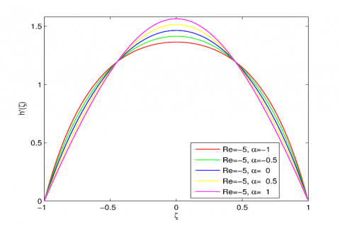
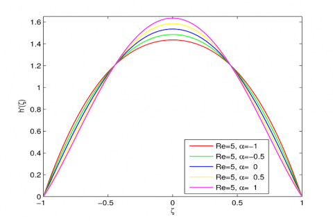
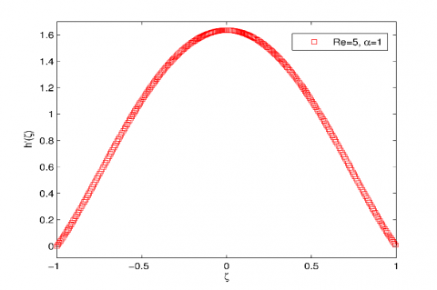
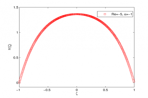
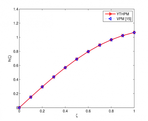
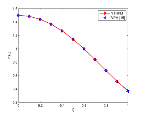
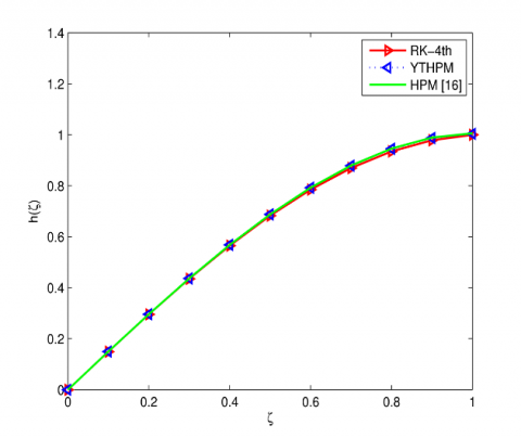
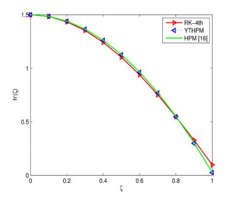
Figures 2, 3 show the effect of various values of α on the derivative of velocity h'(ζ) at Re=-5,5. These figures illustrate the expanding wall (α>0) and contracting wall (α<0) for the suction case (Re=-5) and injection case (Re=5), respectively. Figure 4 explains the effect of different values of α on h'(ζ) at Re=0. Moreover, Figures 5, 6 demonstrate h'(ζ) at α=1, Re=5 and α=-1, Re=-5, and explain the state of expansion combined with injection and the state of contraction combined with suction, respectively. Figure 7 shows the comparison of results between the new method and VPM [15] at Re=5 and α=0.5 for h(ζ) and h'(ζ), respectively for the state of expansion combined with injection. On another note, Figure 8 explains the comparison of the results between, YTHPM, RK-4th order, and HPM [16] for α=0.5 and Re=1 for h(ζ) and h'(ζ), respectively.
Figure 2. The influence of various values of α on the derivative of velocity h'(ζ) at Re=-5
Figure 3. The influence of various values of α on the derivative of velocity h'(ζ) at Re=5
Figure 4. The influence of various values of α on the derivative of velocity h'(ζ) at Re=0
Figure 5. h'(ζ) at α=1 and Re=5
Figure 6. h'(ζ) at α=-1 and Re=-5
Figure 7. Comparison of results between YTHPM and VPM [15] of flow when α=0.5 and Re=5 for h(ζ) and h'(ζ) respectively
Figure 8. Comparison of results between YTHPM, HPM [16], and RK-4th when α=0.5 and Re=1 for h(ζ) and h'(ζ) respectively
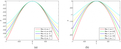
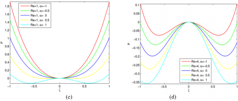
After we find the flow field, the remaining important properties of the flow like the pressure and shear stress can be found as follows: The gradient of pressure can be found by putting the components of velocity in Eq. (24). Then:
P_{\zeta}=-\left(\frac{1}{\operatorname{Re}} h_{\zeta \zeta}+h h_{\zeta}+\frac{\alpha}{\operatorname{Re}}\left[h+\zeta h_{\zeta}\right]\right) ; \quad P=\frac{\ddot{P}}{\rho U_{w}^{2}} (36)
The normal distribution of pressure can be found through integrating Eq. (36). The pressure distributions are plots for different values of Re, as illustrated in Figure 9. Also, we observe that the pressure term changes for each level of suction or injection and becomes the lowest level near the central part.
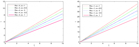
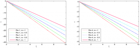
The shear stress is the other important quantity, which can be specified from Newton’s law for viscosity:
\dddot{\tau}=\left(\dddot{v}_{\dddot{x}}+\dddot{u}_{\dddot{y}}\right)=\frac{\rho v^{2} \dddot{x} \dddot{h}_{\dddot{y y}}}{a^{3}} (37)
The non-dimensional shear stress is defined as: \tau=\frac{\dddot{\tau}}{\rho U_{w}^{2}}, then:
\tau =\frac{x\,{{h}_{\zeta \zeta }}}{\operatorname{Re}} (38)
The wall shear stress \left( \tau =\frac{x\,{{h}_{\zeta \zeta }}(1)}{\operatorname{Re}} \right) is plotted at various values of Re and α, as shown in Figure 10. It should be noted that the shear stress increases over the length of the wall surface. Moreover, when α decreases, the wall shear stress increases as the wall is expanding (α>0), but it increases as α increases as the wall is contracting (α<0).
Figure 9. The pressure distribution (a-d) at various values of Re over a rate of α
Figure 10. Shear stress over a range of α and different values of Re
In this part, which is concerned with convergence analysis, we will study the convergence for the analytical approximate solution (35) obtained by using the new method (YTHPM) and as follows:
Definition: Assume that X1 is the Banach space and N: X_{1} \rightarrowℝ is a nonlinear mapping where ℝ is the real numbers. Then, the sequence of the solutions can be written in the following form:
{{W}_{m}}=N({{W}_{m-1}}),\quad {{W}_{m-1}}=\sum\limits_{i=0}^{m-1}{{{w}_{i}}},\quad m=1,2,3,... (39)
where, N satisfies the Lipschitz condition such that \forall \gamma \inℝ.
\left\| N({{W}_{m}})-N({{W}_{m-1}}) \right\|\le \,\gamma \,\left\| {{W}_{m}}-{{W}_{m-1}} \right\|\quad ,0<\gamma <1. (40)
Theorem (1): The series of analytical approximate solutions h=\sum\limits_{k=0}^{\infty }{{{h}_{k}}(\zeta )} obtained from the YTHPM converges if it satisfies the following condition: \left\|W_{m}-W_{n}\right\| \rightarrow 0 when n \rightarrow \infty, 0<\gamma<1.
Proof:
\begin{aligned}\left\|W_{m}-W_{n}\right\| &=\left\|\sum_{i=0}^{m} w_{i}-\sum_{i=0}^{n} w_{i}\right\| \\ &=\left\|w_{0}+\sum_{i=1}^{m} N\left(w_{i}^{\bullet}\right)-w_{0}+\sum_{i=1}^{n} N\left(w_{i}^{\bullet}\right)\right\| \end{aligned},
=\left\|\sum_{i=1}^{m} N\left(w_{i}^{\bullet}\right)+\sum_{i=1}^{n} N\left(w_{i}^{\bullet}\right)\right\|, \quad W_{m}=N\left(W_{m-1}\right)
=\left\|N\left(\sum_{i=0}^{m-1} w_{i}\right)+N\left(\sum_{i=0}^{n-1} w_{i}\right)\right\|
\leq \gamma\left\|W_{m-1}-W_{n-1}\right\|
Because N satisfies the Lipschitz condition and
w_{i}^{\bullet }=\sum\limits_{j=0}^{n}{\int\limits_{0}^{\zeta }{\left( \begin{align} & \alpha \,\left( \zeta \frac{{{\partial }^{3}}{{h}_{j}}}{\partial {{\zeta }^{3}}}+3\frac{{{\partial }^{2}}{{h}_{j}}}{\partial {{\zeta }^{2}}} \right)+ \\ & \operatorname{Re}\sum\limits_{k=0}^{j}{\left( {{h}_{k}}\frac{{{\partial }^{3}}{{h}_{j-k}}}{\partial {{\zeta }^{3}}}-\left( \frac{\partial {{h}_{k}}}{\partial \zeta } \right)\frac{{{\partial }^{2}}{{h}_{j-k}}}{\partial {{\zeta }^{2}}} \right)} \\ \end{align} \right)}}\,d\zeta .
Let, m=n+1 then, we have \left\| {{W}_{n+1}}-{{W}_{n}} \right\|\le \gamma \ \left\| {{W}_{n}}-{{W}_{n-1}} \right\|, then
\left\| {{W}_{n}}-{{W}_{n-1}} \right\|\le \gamma \ \left\| {{W}_{n-1}}-{{W}_{n-2}} \right\|\le \cdots \le {{\gamma }^{n-1}}\ \left\| {{W}_{1}}-{{W}_{0}} \right\| (41)
From (41), we have:
\begin{align} & \left\| {{W}_{2}}-{{W}_{1}} \right\|\le \gamma \ \left\| {{W}_{1}}-{{W}_{0}} \right\| \\ & \left\| {{W}_{3}}-{{W}_{2}} \right\|\le {{\gamma }^{2}}\ \left\| {{W}_{1}}-{{W}_{0}} \right\| \\ & \vdots \\ & \left\| {{W}_{n}}-{{W}_{n-1}} \right\|\le {{\gamma }^{n-1}}\ \left\| {{W}_{1}}-{{W}_{0}} \right\| \\ \end{align}
By using the triangle inequality, we get:
\begin{align} & \left\| {{W}_{m}}-{{W}_{n}} \right\|=\left\| {{W}_{m}}-{{W}_{m-1}}-\cdots -{{W}_{n+1}}-{{W}_{n}} \right\| \\ & \quad \quad \quad \quad \le \ \left\| {{W}_{m}}-{{W}_{m-1}} \right\|+\left\| {{W}_{m-1}}-{{W}_{m-2}} \right\|+\cdots +\left\| {{W}_{n+1}}-{{W}_{n}} \right\| \\ & \quad \quad \quad \quad \le \left( {{\gamma }^{m-1}}+{{\gamma }^{m-2}}+\cdots +{{\gamma }^{n}} \right)\,\left\| {{W}_{1}}-{{W}_{0}} \right\| \\ & \quad \quad \quad \quad \le \frac{{{\gamma }^{n}}}{1-\gamma }\left\| {{W}_{1}}-{{W}_{0}} \right\| \\ \end{align}
when, n \rightarrow \infty we have \left\|W_{m}-W_{n}\right\| \rightarrow 0, then Wm is the Cauchy sequence in Banach space X1.
Theorem (2): The solution by the new method (YTHPM) h=\sum\limits_{k=0}^{\infty }{{{h}_{k}}(\zeta )} converges and is close to the solution problem (32-33) if the following property is achieved:
{{L}^{-1}}N\left( h \right)=\underset{m\to \infty }{\mathop{\lim }}\,\,{{L}^{-1}}N\left( {{W}_{m}} \right), where {{L}^{-1}}(*)=\int\limits_{0}^{\zeta }{(*)d\zeta }.
Proof: For any W \in X_{1} define an operator from X1 to X1, \ell(W)=W_{0}+L^{-1} N(W).
Let, W_{1}, W_{2} \in X_{1}, then we have:
\begin{align} & \left\| \ell ({{W}_{1}})-\ell ({{W}_{2}}) \right\|=\left\| {{W}_{0}}+{{L}^{-1}}N({{W}_{1}})-{{W}_{0}}-{{L}^{-1}}N({{W}_{2}}) \right\| \\ & \quad \quad \quad \quad \quad \ \ =\left\| {{L}^{-1}}N({{W}_{1}})-{{L}^{-1}}N({{W}_{2}}) \right\| \\ & \quad \quad \quad \quad \quad \ \ \le \left| {{L}^{-1}} \right|\,\left\| N({{W}_{1}})-N({{W}_{2}}) \right\| \\ & \quad \quad \quad \quad \quad \ \ \le \gamma \,\left\| {{W}_{1}}-{{W}_{2}} \right\| \\ \end{align}
Therefore, the mapping \ell is contractive, and Banach fixed point theorem for contractive offers a unique solution for the problem (32-33). Now, we prove that the series solution h(\zeta ) satisfies problem (32-33):
{{L}^{-1}}N\left( h \right)={{L}^{-1}}N\left( \sum\limits_{k=0}^{\infty }{{{h}_{k}}} \right)={{L}^{-1}}N\left( \underset{m\to \infty }{\mathop{\lim }}\,\sum\limits_{i=0}^{n}{{{w}_{i}}} \right) ={{L}^{-1}}N\left( \,\underset{m\to \infty }{\mathop{\lim }}\,{{W}_{m}} \right)=\underset{m\to \infty }{\mathop{\lim }}\,\,{{L}^{-1}}N\left( {{W}_{m}} \right)
From Theorems (1) and (2), the values of the parameter γm must be calculated to obtain convergence by using the following relationship:
{{\gamma }^{m}}=\left\{ \begin{align} & \frac{\left\| \,{{W}_{m+1}}-{{W}_{m}} \right\|}{\left\| {{W}_{1}}-{{W}_{0}} \right\|}=\frac{\left\| {{h}_{m+1}} \right\|}{\left\| {{h}_{1}} \right\|},\quad \left\| {{h}_{1}} \right\|\ne 0,\quad m=1,2,3,\cdots \\ & 0,\quad \quad \quad \quad \quad \quad \quad \quad \left\| {{h}_{1}} \right\|=0 \\ \end{align} \right.
Now, by using this definition, we find the convergence of the problem as follows:
\left\|h_{1}-h_{0}\right\|=\|\left(\begin{array}{l}\frac{\alpha}{10} \zeta-\frac{\alpha}{5} \zeta^{3}+\frac{\alpha}{10} \zeta^{5}+\frac{\operatorname{Re}}{140} \zeta- \\ \frac{3 \operatorname{Re}}{280} \zeta^{3}+\frac{\operatorname{Re}}{280} \zeta^{7}-\frac{\alpha \operatorname{Re}}{63567504000} \zeta^{7} \\ +\frac{\alpha \operatorname{Re}}{1149603840} \zeta^{9}+\ldots\end{array}\right)-\left(\frac{3}{2} \zeta-\frac{1}{2} \zeta^{3}\right)
\left\|h_{2}-h_{1}\right\| \leq\left\|h_{1}-h_{0}\right\| \gamma, \quad \gamma=0.000362<1, \\ \left\|h_{3}-h_{2}\right\| \leq\left\|h_{1}-h_{0}\right\| \gamma^{2}, \quad \gamma^{2}=0.00003089<1 \\ \vdots \\ \left\|h_{m}-h_{m-1}\right\| \leq\left\|h_{1}-h_{0}\right\| \gamma^{m}.
We have proposed in this research a new technique called the Yang transform homotopy perturbation method (YTHPM) to solve the two-dimensional (2D) incompressible viscous fluid flow problems among two slowly expand or contract walls. The results which we obtained by using Mathcad.15 to solve this problem show that YTHPM is an efficacious method with high accuracy to find analytical approximate solutions to this problem. Also, we noted that for each level of injection or suction, when the wall is expanding (α>0), an increase α lead up to the velocity becomes higher close to the center and lower near the wall. This happens because the flow becomes larger toward the center to compensate the area resulting from the expansion of the wall. As a result, the velocity also becomes larger close to the center. Also, for all levels of suction or injection, if the wall is contracting (α<0), increase α lead to the axial velocity becomes low close to the center and high near the wall, the reason that the velocity becomes larger close to the wall because the flow towards the wall becomes larger. Moreover, from the comparison between the new method [4, 15, 16], we note that this method is effective and powerful, also its results agree well with the results of these methods. Although there is an agreement between the methods, the new technique is preferred. We obtained our results through the 1st iteration, but in ref. [4], the results are acquired by the 10th -order approximation. In ref. [16], results are obtained from the 4th iteration and in ref. [15] from the 15th iteration. Then, we conclude that the YTHPM is an efficient and highly accurate method for finding the analytical approximate solution of the two-dimensional viscous fluid flow problem among two slowly expanding or contracting walls and can be used as well to find the analytical approximate solutions for different fluid flow problems.
[1] Berman, A.S. (1953). Laminar flow in channels with porous walls. Journal of Applied Physics, 24(9): 1232-1235. https://doi.org/10.1063/1.1721476
[2] Ganji, Z.Z., Ganji, D.D., Janalizadeh, A. (2010). Analytical solution of two-dimensional viscous flow between slowly expanding or contracting walls with weak permeability. Mathematical and Computational Applications, 15(5): 957-961. https://doi.org/10.3390/mca15050957
[3] Dinarvand, S. (2012). Reliable treatments of differential transform method for two-dimensional incompressible viscous flow through slowly expanding or contracting porous walls with small-to-moderate permeability. International Journal of the Physical Sciences, 7(8): 1166-1174. http://dx.doi.org/10.5897/IJPS11.1753
[4] Dinarvand, S., Rashidi, M., Doosthoseini, A. (2009). Analytical approximate solutions for two-dimensional viscous flow through expanding or contracting gaps with permeable walls. Open Physics, 7(4): 791-799. https://doi.org/10.2478/s11534-009-0024-x
[5] Sushila, Singh, J., Shishodia, Y.S. (2014). A reliable approach for two-dimensional viscous flow between slowly expanding or contracting walls with weak permeability using sumudu transform. Ain Shams Engineering Journal, 5(1): 237-242. https://doi.org/10.1016/j.asej.2013.07.001
[6] Ledari, S.T., Mirgolbabaee, H.H., Domiri Ganji, D. (2015). An assessment of a semi analytical AG method for solving two-dimension nonlinear viscous flow. International Journal of Nonlinear Analysis and Applications, 6(2): 47-64. https://dx.doi.org/10.22075/ijnaa.2015.270
[7] Yang, X.J. (2016). A new integral transform method for solving steady heat-transfer problem. Thermal Science, 20(s3): 639-642.
[8] Yang, X.J., Gao, F. (2017). A new technology for solving diffusion and heat equations. Thermal Science, 21(1 Part A): 133-140.
[9] Dattu, M.K.U. (2018). New integral transform: Fundamental properties, investigations and applications. IAETSD Journal for Advanced Research in Applied Sciences, 5(4): 534-539.
[10] Aminikhah, H., Hemmatnezhad, M. (2010). An efficient method for quadratic Riccati differential equation. Communications in Nonlinear Science and Numerical Simulation, 15(4): 835-839. https://doi.org/10.1016/j.cnsns.2009.05.009
[11] Mirzazadeh, M., Ayati, Z. (2016). New homotopy perturbation method for system of Burgers equations. Alexandria Engineering Journal, 55(2): 1619-1624. https://doi.org/10.1016/j.aej.2016.02.003
[12] Rubab, S., Ahmad, J., Naeem, M. (2014). Exact solution of klein gordon equation via homotopy perturbation sumudu transform method. International Journal of Hybrid Information Technology, 7(6): 445-452. http://dx.doi.org/10.14257/ijhit.2014.7.6.38
[13] Debnath, L., Bhatta, D. (2014). Integral Transforms and Their Applications. CRC Press, Boca Raton, Fla., USA.
[14] Majdalani, J., Zhou, C., Dawson, C.A. (2002). Two-dimensional viscous flow between slowly expanding or contracting walls with weak permeability. Journal of Biomechanics, 35(10): 1399-1403. https://doi.org/10.1016/S0021-9290(02)00186-0
[15] Sobamowo, G.M. (2017). On the analysis of laminar flow of viscous fluid through a porous channel with suction/injection at slowly expanding or contracting walls. Journal of Computational Applied Mechanics, 48(2): 319-330.
[16] Yahyazadeh, A., Yahyazadeh, H., Khalili, M., Malekzadeh, M. (2012). Analytical solution of two-dimensional viscous flow between slowly expanding or contracting walls with weak permeability. Journal of Mathematics and Computer Science, 5(4): 331-336. http://dx.doi.org/10.22436/jmcs.05.04.11