Razon Kumar Mondal | Sheikh Reza-E-Rabbi* | Partha Protim Gharami | Sarder Firoz Ahmmed | Shikdar Mohammad Arifuzzaman
OPEN ACCESS
This article is related with the simulation of mass and heat relocation behavior of viscous dissipative chemically reacted Casson fluid which is flowing with impact of suction, thermal conductivity and fickle viscosity. Current conductivity along with temperature dependent viscosity changes as a linear function of temperature. First of all, leading equations are converted into dimensionless form via suitable transformations. Therefore explicit finite differential technique has solved the obtained non-dimensional, non-similar mixed non-linear and partial differential equations with the support of Compaq Visual Fortran 6.6.a, a very well-known programing language. The behavior of various relevant parameters in the boundary profile velocity, temperature and concentration was considered realistically. Therefore, these variables have a diagrammatic influence on skin friction and the heat transference coefficient profiles. Stability and convergence tests are also carried out for the accuracy of implemented numerical scheme. One of the significant attainment is the Casson fluid parameter displayed quite interesting behavior on the velocity fields as it represented provoking behavior close to the boundary but it behaved oppositely away from the boundary surface. However, a comparison is also presented with good agreement for the validation of the current investigation.
Casson fluid, chemical reaction, porous medium, explicit finite difference method, MHD
The learning of non-Newtonian liquid has fascinated a lot of attention due to their intensive form of solicitations in production and business particularly in abstraction of fossil fuel from unpolished product, fabrication of plastic resources and treacle drags. Within class of viscous liquids, Casson liquid takes dissimilar options. Casson liquid is single amongst the categories of such viscous liquids that performs alike pliable compacted, and there is a vintage shear stress within the essential equation aimed at this type of liquid. Non-Newtonian transference phenomena ascend in several twigs of motorized and chemical manufacturing and conjointly in sustenance process. The possessions of non- Newtonian liquid are displayed by some usual materials that include shampoos, glues, tomato pastes, milk, sugar solutions, ink etc. In his research, Casson [1] depicted this rheological model on a drift calculation for tint oil-suspensions of lithography toner. Casson model is a model of elastic liquid that shows characteristics of shear slicing, produce stress, and large viscosity of shear. Following the study shown by Rao et al. [2] it's declared that Casson liquid exemplary is condensed to non-viscous liquid at an awfully large wall trim pressure, i.e., once the hassle on the wall exceeds the stress yield. This liquid archetypal also estimates rationally glowing the rheological performance of additional waters together with biological suspensions, froths, cosmetics, sauces, etc. While completing different facsimiles are projected to clarify the conduct of non-Newtonian liquids, the foremost necessary non-Newtonian liquid having a produce rate is that the Casson liquid. Bird et al. [3] scrutinized rheology then drift of viscous-plastic ingredients and recounted that Casson archetypal organizes a plastic liquid prototypical which reveals shear retreating features, produce trauma, and large shear stickiness. Evan Mitsoulis [4] addressed the stress-deformation behavior of viscoelastic models and various constituent equations in detail in 2007. However, several significant problems regarding viscoelastic flows such as flows around a sphere, entry and exit flows from dies were also reviewed by Mitsoulis. Mukhopadhyay [5] described the temperature transmission phenomena of non-Newtonian liquid which is flowing on a stretched shallow. Hayat et al. [6] studied Dufour and Soret impacts on MHD drift of Casson liquid. The heat transmission attitude of a time dependent Casson liquid flowing concluded a movable plane plate with permitted rivulet were considered by Mustafa et al. [7] and explained the problematic systematically via Homotopy investigation method (HAM). Chemical retort is processed that maintain the renovation of one usual of chemical elements to another. Chemical retort and soret impacts on hydro magnetic micropolar fluid laterally a distending sheet have been studied by Mishra et al. [8]. Radioactivity and chemical retort impacts on MHD Casson liquid movement through a wavering erect plate implanted in permeable intermediate was studied by Katarial and Patel [9]. The influence of cross diffusion as well as mass and heat transmission of various hydromagnetic fluid flows resulting from a stretching sheet and an oscillatory vertical plate have been depicted with the impression of higher order chemical reaction by following authors [10-12]. A convergence scheme has been established in their work. For details one can refer the following articles [13-15]. Hayat et al. [16] inspected the flow movement of a fluid which has linear relation between stress and strain with diverse physical aspect. Moreover, Xuan and Roetzel [17] considered the fluid which maintain the similar relation and pursued the analysis with nanoparticles. However, the following authors [18-22] explored the heat transfer improvement of several base fluid along with nano particles by imposing the R-K basis shooting technique. The fluids which maintain non-linear relation between stress and strain are also being apprehended in their research.
The main impartial of the extant paper is to learning the properties of flexible viscosity and updraft conductivity on unstable permitted convective fever and corpus transmission Casson fluid drift with pressure and chemical rejoinder. We have extended the work of IL Animasaun [11]. He has deliberated steady case in their experimental work but we have considered unsteady case in our present paper. We have used a usual transformation in our investigation and solve our difficult numerically by exhausting explicit finite changed scheme. The outcomes are figured for several physical factors with the support of computer indoctrination languages Compaq Visual Fortran 6.6.a and the gained outcomes are strategized afterward stability investigation via graphics software Tecplot-9.
An unsteady 2D laminar permitted convective mass and heat transference viscid incompressible fickle viscosity and inconstant updraft conductivity Casson fluid drift with force and chemical antiphon is considered. The superficial is supposed to remain flexible; the indication of an incompressible liquid is evoked due to enlarging possessions and resilience. This happens in sight of pliable things of the superficial analogous to lx=0 concluded alike and opposed forces once the source is stable at x=y=0. During this analysis, lx-axis is engaged on way of salver and ly-axis is ordinary to it. It remains supposed tthat an unvarying magnetic arena of forte B0 is realistic in erect way near the stream. In this study, the rheological equation for Casson fluid flow stays considered as [5]
$\left. \begin{matrix} {{T}_{ij}}=2\left( {{\mu }_{b}}+\frac{{{P}_{y}}}{\sqrt{2\pi }} \right){{e}_{ij}}\text{ When, }\pi >\text{}{{\pi }_{c}} \\ {{T}_{ij}}=2\left( {{\mu }_{b}}+\frac{{{P}_{y}}}{\sqrt{2\pi }} \right){{e}_{ij}}\text{ When, }\pi <{{\pi }_{c}} \\ \end{matrix} \right\}$
${{P}_{y}}$ is produce shear stress and known as, ${{P}_{y}}=\frac{{{\mu }_{b}}\sqrt{2\pi }}{\beta }$.
Here, ${{\mu }_{b}}$ is non-Newtonian plastic dynamic viscosity and $\pi $ is multiple rate of deformity itself. Also, Tij is the component of stress tension and eijis the (i, j)th component of the deformation rate. In case of non-Newtonian drift where $\pi >{{\pi }_{c}}$ and $\mu ={{\mu }_{b}}+\frac{{{P}_{y}}}{\sqrt{2\pi }}$. Then kinematic viscosityl can be formed as,
$\nu =\frac{{{\mu }_{b}}}{\rho }\left( 1+\frac{1}{\beta } \right)$
Under these following assumptions the formulas are taken regulating the mass, momentum, energy and concentration
$\frac{\partial {u}'}{\partial {x}'}+\frac{\partial {v}'}{\partial {y}'}=0$ (1)
$\begin{align} & \frac{\partial {u}'}{\partial {t}'}+{u}'\frac{\partial {u}'}{\partial {x}'}+{v}'\frac{\partial {u}'}{\partial {y}'}=g\beta \left( {T}'-{{{{T}'}}_{\infty }} \right)+g{{\beta }^{*}}\left( {C}'-{{{{C}'}}_{\infty }} \right) \\ & +\frac{1}{\rho }\left( 1+\frac{1}{\beta } \right)\frac{\partial }{\partial {y}'}\left( {{\mu }_{B}}\frac{\partial {u}'}{\partial {y}'} \right)-\vartheta \frac{{{u}'}}{K}-\frac{\sigma B_{0}^{2}{u}'}{\rho } \\ \end{align}$ (2)
$\begin{align} & \frac{\partial {T}'}{\partial {t}'}+{u}'\frac{\partial {T}'}{\partial {x}'}+{v}'\frac{\partial {T}'}{\partial {y}'}=\frac{1}{\rho {{C}_{p}}}\frac{\partial }{\partial {y}'}\left( \kappa \frac{\partial {T}'}{\partial {y}'} \right)+\frac{\vartheta }{{{C}_{p}}}{{\left( \frac{\partial {u}'}{\partial {y}'} \right)}^{2}} \\ & +\frac{D{{K}_{t}}}{{{C}_{p}}{{C}_{s}}}\frac{{{\partial }^{2}}{C}'}{\partial {{{{y}'}}^{2}}} \\ \end{align}$ (3)
$\frac{\partial {C}'}{\partial {t}'}+{u}'\frac{\partial {C}'}{\partial {x}'}+{v}'\frac{\partial {C}'}{\partial {y}'}=D\frac{{{\partial }^{2}}{C}'}{\partial {{{{y}'}}^{2}}}-R*\left( {C}'-{{{{C}'}}_{\infty }} \right)$ (4)
Subject to the following boundary conditions
$\left. \begin{align} & {u}'={{U}_{w}},\,{v}'=-{{V}_{w}},\,{T}'={{{{T}'}}_{w}},\,\,{C}'={{{{C}'}}_{w}}\,\,\text{at}\,\,{y}'=0 \\ & {u}'\to 0,\,{C}'\to {{{{C}'}}_{\infty }},\,{T}'\to {{{{T}'}}_{\infty }}\,\,\,\,\,\,\,\,\,\,\,\,\,\,\,\,\,\,\,\text{as}\,{y}'\to \infty \\ \end{align} \right\}$ (5)
Since, the explanation of the leading equations underneath the preliminary and frontier settings have been constructed on the finite transformation scheme. So, to make the equations dimensionless, it is necessary. Variables without proportions can be represented as,
$\begin{align} & U=\frac{{{u}'}}{{{U}_{0}}},V=\frac{{{v}'}}{{{U}_{0}}},X=\frac{{x}'{{U}_{0}}}{\vartheta },Y=\frac{{y}'{{U}_{0}}}{\vartheta },{{S}_{c}}=\frac{\nu }{D},M=\frac{\sigma B_{0}^{2}\nu }{\rho U_{0}^{2}}, \\ & {{K}_{r}}=\frac{\vartheta R}{U_{0}^{2}},{x}'=\frac{X\vartheta }{{{U}_{0}}}{y}'=\frac{Y\vartheta }{{{U}_{0}}},\tau =\frac{{t}'U_{0}^{2}}{\vartheta },\theta =\frac{{T}'-{{{{T}'}}_{\infty }}}{{{{{T}'}}_{w}}-{{{{T}'}}_{\infty }}},C=\frac{{C}'-{{{{C}'}}_{\infty }}}{{{{{C}'}}_{w}}-{{{{C}'}}_{\infty }}}, \\ & k=\frac{U_{0}^{2}{K}'}{{{\vartheta }^{2}}},{{P}_{r}}=\frac{\rho \vartheta {{C}_{p}}}{\kappa },{{G}_{r}}=\frac{g\beta \vartheta ({{{{T}'}}_{w}}-{{{{T}'}}_{\infty }})}{U_{0}^{3}},{{G}_{m}}=\frac{g\beta *\vartheta ({{{{C}'}}_{w}}-{{{{C}'}}_{\infty }})}{U_{0}^{3}}, \\ & {{E}_{c}}=\frac{U_{0}^{2}}{{{C}_{p}}\left( {{{{T}'}}_{w}}-{{{{T}'}}_{\infty }} \right)},{{D}_{f}}=\frac{{{D}_{m}}{{K}_{T}}\left( {{{{C}'}}_{w}}-{{{{C}'}}_{\infty }} \right)}{{{C}_{p}}{{C}_{s}}\vartheta \left( {{{{T}'}}_{w}}-{{{{T}'}}_{\infty }} \right)} \\ \end{align}$
Here,
$\mu ={{\mu }_{0}}\left( a+\lambda \left( {T}'-{{{{T}'}}_{\infty }} \right) \right)$ and $\kappa ={{\kappa }_{0}}\left( a+\delta \left( {T}'-{{{{T}'}}_{\infty }} \right) \right)$
Let $\gamma $ and $\varepsilon $ denote the non-dimensional parameter of variation of viscosity and thermal conductivity be considered by $\gamma =\lambda \left( {{{{T}'}}_{w}}-{{{{T}'}}_{\infty }} \right)$ and $\varepsilon =\delta \left( {{{{T}'}}_{w}}-{{{{T}'}}_{\infty }} \right)$.
The corresponding form is then provided by the liquid viscosity and fervor conductivity
$\mu ={{\mu }_{0}}\left( a+\gamma T \right)\,\,\text{and}\,\,\kappa ={{\kappa }_{0}}\left( a+\varepsilon T \right)$ (6)
$\frac{\partial U}{\partial X}+\frac{\partial V}{\partial Y}=0$ (7)
$\begin{align} & \frac{\partial U}{\partial \tau }+U\frac{\partial U}{\partial X}+V\frac{\partial U}{\partial Y}={{G}_{r}}\theta +{{G}_{m}}C+\left( 1+\frac{1}{\beta } \right) \\ & \left( \frac{\gamma }{a+\gamma \theta } \right)\frac{\partial \theta }{\partial Y}\frac{\partial U}{\partial Y}+\left( 1+\frac{1}{\beta } \right)\frac{{{\partial }^{2}}U}{\partial {{Y}^{2}}}-\frac{U}{k}-MU \\ \end{align}$ (8)
$\begin{align} & \frac{\partial \theta }{\partial \tau }+U\frac{\partial \theta }{\partial X}+V\frac{\partial \theta }{\partial Y}=\frac{1}{{{P}_{r}}}\left( \frac{{{\partial }^{2}}\theta }{\partial {{Y}^{2}}}+\frac{\varepsilon }{a+\varepsilon \theta }{{\left( \frac{\partial \theta }{\partial Y} \right)}^{2}} \right) \\ & +\left( 1+\frac{1}{\beta } \right){{E}_{c}}{{\left( \frac{\partial U}{\partial Y} \right)}^{2}}+{{D}_{f}}\frac{{{\partial }^{2}}C}{\partial {{Y}^{2}}} \\ \end{align}$ (9)
$\frac{\partial C}{\partial \tau }+U\frac{\partial C}{\partial X}+V\frac{\partial C}{\partial Y}=\frac{1}{{{S}_{C}}}\frac{{{\partial }^{2}}C}{\partial {{Y}^{2}}}-{{K}_{r}}C$ (10)
With boundary conditions,
$\left. \begin{align} & U=1,V=-1,\theta =1,C=1\,\,\text{at}\,\,Y=0 \\ & U\to 0,\theta \to 0,C\to 0\,\,\,\,\,\,\,\,\,\text{as}\,\,Y\to \infty \\ \end{align} \right\}$ (11)
The physical quantities skin lfriction and heat transfer coefficient are presented at non-dimension form and given by,
${{S}_{f}}=\frac{1}{2\sqrt{2}}{{\left( {{G}_{r}} \right)}^{-\frac{3}{4}}}{{\left( \frac{\partial U}{\partial Y} \right)}_{Y=0}}$ and ${{N}_{u}}=\frac{1}{2\sqrt{2}}{{\left( {{G}_{r}} \right)}^{-\frac{3}{4}}}{{\left( \frac{\partial \theta }{\partial Y} \right)}_{Y=0}}$
To solve the controlling second order, together with the corresponding original and boundary constraints, non-dimensional partial differential equations. According to original and border constraints, process of explicit transformation was recycled to decipher (8)-(11). The area of stream is separated hooked on a lattice or network of outlines similar to X and Y alliance is engaged along platter in order to obtain the differential equations. Here is the tallness plate Xmax=20 i.e. X fluctuates from 0 to 20 and honor Ymax =50 as agreeing to $y\to \infty $ such that Y fluctuates from 0 to 50. Here are n=300 and m=100 gridiron layout in X and Y instructions correspondingly. It remains rumored that $\Delta X$ and $\Delta Y$ are perpetual lattice extents laterally X andl Y instructions correspondingly and reserved as follows, $\Delta Y=0.25\left( 0\le x\le 50 \right)\,\,\text{and}\,\,\Delta X=0.20\left( 0\le x\le 20 \right)\,\,\,\,$with minor time-step, Δ $\tau =0.005$ .
The following are sufficient arrays of finite differences of the governing formulas using the direct finite transformation approximation.
$\frac{{{U}_{i,j}}-{{U}_{i-1,j}}}{\Delta X}+\frac{{{V}_{i,j}}-{{V}_{i,j-1}}}{\Delta Y}=0$ (12)
$\begin{align} & \frac{{{{{U}'}}_{i,j}}-{{U}_{i,j}}}{\Delta \tau }+{{U}_{i,j}}\frac{{{U}_{i,j}}-{{U}_{i-1,j}}}{\Delta X}+{{V}_{i,j}}\frac{{{V}_{i,j}}-{{V}_{i,j-1}}}{\Delta Y}={{G}_{r}}{{\theta }_{i,j}}+ \\ & {{G}_{m}}{{C}_{i,j}}+\left( 1+\frac{1}{\beta } \right)\left( \frac{\gamma }{a+\gamma {{\theta }_{i,j}}} \right)\left( \frac{{{\theta }_{i,j+1}}-{{\theta }_{i,j}}}{\Delta Y} \right)\left( \frac{{{U}_{i,j+1}}-{{U}_{i,j}}}{\Delta Y} \right) \\ & +\left( 1+\frac{1}{\beta } \right)\left( \frac{{{U}_{i,j+1}}-2{{U}_{i,j}}+{{U}_{i,j-1}}}{{{\left( \Delta Y \right)}^{2}}} \right)-\frac{{{U}_{i,j}}}{k}-M{{U}_{i,j}} \\ \end{align}$(13)
$\begin{align} & \frac{{{{{\theta }'}}_{i,j}}-{{\theta }_{i,j}}}{\Delta \tau }+{{U}_{i,j}}\frac{{{\theta }_{i,j}}-{{\theta }_{i-1,j}}}{\Delta X}+{{V}_{i,j}}\frac{{{\theta }_{i,j+1}}-{{\theta }_{i,j}}}{\Delta Y}=\frac{1}{{{P}_{r}}} \\ & \left( \left( \frac{{{\theta }_{i,j+1}}-2{{\theta }_{i,j}}+{{\theta }_{i,j-1}}}{{{\left( \Delta Y \right)}^{2}}} \right) \right.\left. +\left( \frac{\varepsilon }{a+\varepsilon {{\theta }_{i,j}}} \right){{\left( \frac{{{\theta }_{i,j+1}}-{{\theta }_{i,j}}}{\Delta Y} \right)}^{2}} \right) \\ & +\left( 1+\frac{1}{\beta } \right){{E}_{c}}{{\left( \frac{{{U}_{i,j+1}}-{{U}_{i,j}}}{\Delta Y} \right)}^{2}}+{{D}_{f}}\left( \frac{{{C}_{i,j+1}}-2{{C}_{i,j}}+{{C}_{i,j-1}}}{{{\left( \Delta Y \right)}^{2}}} \right) \\ \end{align}$ (14)
$\begin{align} & \frac{{{{{C}'}}_{i,j}}-{{C}_{i,j}}}{\Delta \tau }+{{U}_{i,j}}\frac{{{C}_{i,j}}-{{C}_{i-1,j}}}{\Delta X}+{{V}_{i,j}}\frac{{{C}_{i,j+1}}-{{C}_{i,j}}}{\Delta Y}=\frac{1}{{{S}_{C}}} \\ & \left( \frac{{{C}_{i,j+1}}-2{{C}_{i,j}}+{{C}_{i,j-1}}}{{{\left( \Delta Y \right)}^{2}}} \right)-{{K}_{r}}{{C}_{i,j}} \\ \end{align}$ (15)
The primary and border condition with finite transformation system as,
$\left. \begin{align} & U_{i,0}^{n}=1,V_{i,0}^{n}=-1,\theta _{i,0}^{n}=1,C_{i,0}^{n}=1\,\,\text{when}\,\,Y=0 \\ & U_{i,L}^{n}=0,\theta _{i,L}^{n}=0,C_{i,L}^{n}=0\,\,\,\,\,\,\,\,\,\,\,\,\,\,\,\,\,\,\text{when}\,\,Y\to \infty \\ \end{align} \right\}$ (16)
where, i then j elect to the lattice facts with X and Y synchronize individually and the subscripts n characterizes a significance of time.
Because an explicit metamorphosis method is being implemented, the current enquiry would persist imperfect if we do not exhibit any stability and convergence test. For perpetual lattice extents the stability principle could be established as follows. Because ∆τ is missing in Eq. (12), it will be neglected. For, U, lT and C the overall relations of Fourier extension are all ${{e}^{i\alpha X}}{{e}^{i\beta Y}}$. At period τ we get,
$\left. \begin{align} & U:D\left( \tau \right){{e}^{i\alpha X}}{{e}^{i\beta Y}} \\ & T:E\left( \tau \right){{e}^{i\alpha X}}{{e}^{i\beta Y}} \\ & C:F\left( \tau \right){{e}^{i\alpha X}}{{e}^{i\beta Y}} \\ \end{align} \right\}$ (17)
after a time step
$\left. \begin{align} & U:{D}'\left( \tau \right){{e}^{i\alpha X}}{{e}^{i\beta Y}} \\ & T:{E}'\left( \tau \right){{e}^{i\alpha X}}{{e}^{i\beta Y}} \\ & C:{F}'\left( \tau \right){{e}^{i\alpha X}}{{e}^{i\beta Y}} \\ \end{align} \right\}$ (18)
Considering U, V as constants and using Eqns. (17), (18) in Eqns. (13)-(15) we get,
$\begin{align} & \frac{\left( {D}'-D \right){{e}^{i\alpha X}}{{e}^{i\beta Y}}}{\Delta \tau }+U\frac{D{{e}^{i\alpha X}}{{e}^{i\beta Y}}\left( 1-{{e}^{-i\alpha \Delta X}} \right)}{\Delta X}+V\frac{D{{e}^{i\alpha X}}{{e}^{i\beta Y}}\left( {{e}^{i\beta \Delta Y}}-1 \right)}{\Delta Y} \\ & ={{G}_{r}}E{{e}^{i\alpha X}}{{e}^{i\beta Y}}+{{G}_{m}}F{{e}^{i\alpha X}}{{e}^{i\beta Y}}+\left( 1+\frac{1}{\beta } \right)\left( \frac{\gamma }{a+\gamma E{{e}^{i\alpha X}}{{e}^{i\beta Y}}} \right) \\ & \left( \frac{E{{e}^{i\alpha X}}{{e}^{i\beta Y}}\left( {{e}^{i\beta \Delta Y}}-1 \right)}{\Delta Y} \right)\left( \frac{D{{e}^{i\alpha X}}{{e}^{i\beta Y}}\left( {{e}^{i\beta \Delta Y}}-1 \right)}{\Delta Y} \right) \\ & +\left( 1+\frac{1}{\beta } \right)\frac{2D{{e}^{i\alpha X}}{{e}^{i\beta Y}}\left( \cos \beta \Delta Y-1 \right)}{{{\left( \Delta Y \right)}^{2}}}-MD{{e}^{i\alpha X}}{{e}^{i\beta Y}} \\ & -\frac{1}{k}D{{e}^{i\alpha X}}{{e}^{i\beta Y}} \\ \end{align}$ (19)
$\begin{align} & \frac{\left( {E}'-E \right){{e}^{i\alpha X}}{{e}^{i\beta Y}}}{\Delta \tau }+U\frac{E{{e}^{i\alpha X}}{{e}^{i\beta Y}}\left( 1-{{e}^{-i\alpha \Delta X}} \right)}{\Delta X} \\ & +V\frac{E{{e}^{i\alpha X}}{{e}^{i\beta Y}}\left( {{e}^{i\beta \Delta Y}}-1 \right)}{\Delta Y}=\frac{1}{{{P}_{r}}}\left\{ \frac{2E{{e}^{i\alpha X}}{{e}^{i\beta Y}}\left( \cos \beta \Delta Y-1 \right)}{{{\left( \Delta Y \right)}^{2}}} \right. \\ & \left. +\frac{\varepsilon }{a+\varepsilon E{{e}^{i\alpha X}}{{e}^{i\beta Y}}}{{\left( \frac{E{{e}^{i\alpha X}}{{e}^{i\beta Y}}\left( {{e}^{i\beta \Delta Y}}-1 \right)}{\Delta Y} \right)}^{2}} \right\} \\ & +\left( 1+\frac{1}{\beta } \right){{E}_{c}}{{\left( \frac{D{{e}^{i\alpha X}}{{e}^{i\beta Y}}\left( {{e}^{i\beta \Delta Y}}-1 \right)}{\Delta Y} \right)}^{2}} \\ & +{{D}_{f}}\frac{2F{{e}^{i\alpha X}}{{e}^{i\beta Y}}\left( \cos \beta \Delta Y-1 \right)}{{{\left( \Delta Y \right)}^{2}}} \\ \end{align}$ (20)
$\begin{align} & \frac{\left( {F}'-F \right){{e}^{i\alpha X}}{{e}^{i\beta Y}}}{\Delta \tau }+U\frac{F{{e}^{i\alpha X}}{{e}^{i\beta Y}}\left( 1-{{e}^{-i\alpha \Delta X}} \right)}{\Delta X} \\ & +V\frac{F{{e}^{i\alpha X}}{{e}^{i\beta Y}}\left( {{e}^{i\beta \Delta Y}}-1 \right)}{\Delta Y}=\left( \frac{1}{{{S}_{c}}} \right) \\ & \frac{2F{{e}^{i\alpha X}}{{e}^{i\beta Y}}\left( \cos \beta \Delta Y-1 \right)}{{{\left( \Delta Y \right)}^{2}}}-KrF{{e}^{i\alpha X}}{{e}^{i\beta Y}} \\ \end{align}$ (21)
Thus, Eqns. (19), (20) and (21) can be written as,
$\left. \begin{align} & {D}'={{A}_{1}}D \\ & {E}'={{A}_{2}}E+{{A}_{3}}D \\ & {F}'={{A}_{4}}F+{{A}_{5}}E \\ \end{align} \right\}$ (22)
where,
$\begin{align} & {{A}_{1}}=1+\left( 1+\frac{1}{\beta } \right)\left( \frac{\gamma \theta }{a+\gamma \theta } \right)\frac{\Delta \tau }{{{\left( \Delta Y \right)}^{2}}}{{\left( {{e}^{i\beta \Delta Y}}-1 \right)}^{2}} \\ & +\left( 1+\frac{1}{\beta } \right)\frac{2\Delta \tau }{{{\left( \Delta Y \right)}^{2}}}\left( \cos \beta \Delta Y-1 \right)-M\Delta \tau -\,\frac{\Delta \tau }{k} \\ & -U\frac{\Delta \tau }{\Delta X}\left( 1-{{e}^{-i\alpha \Delta X}} \right)-V\frac{\Delta \tau }{\Delta Y}\left( {{e}^{i\beta \Delta Y}}-1 \right) \\ \end{align}$
${{A}_{2}}={{G}_{r}}\Delta \tau $
${{A}_{3}}={{G}_{m}}\Delta \tau $
$\begin{align} & {{A}_{4}}=1+\frac{1}{Pr}\frac{2\Delta \tau }{{{\left( \Delta Y \right)}^{2}}}\left( \cos \beta \Delta Y-1 \right)+\frac{1}{Pr}\left( \frac{\varepsilon \theta }{a+\varepsilon \theta } \right) \\ & \frac{\Delta \tau }{{{\left( \Delta Y \right)}^{2}}}{{\left( {{e}^{i\beta \Delta Y}}-1 \right)}^{2}}-\,U\frac{\Delta \tau }{\Delta X}\left( 1-{{e}^{-i\alpha \Delta X}} \right)-V\frac{\Delta \tau }{\Delta Y}\left( {{e}^{i\beta \Delta Y}}-1 \right) \\ \end{align}$
${{A}_{5}}=\left( 1+\frac{1}{\beta } \right){{E}_{c}}\frac{\Delta \tau }{{{\left( \Delta Y \right)}^{2}}}{{\left( {{e}^{i\beta \Delta Y}}-1 \right)}^{2}}$
${{A}_{6}}={{D}_{f}}\frac{2\Delta \tau }{{{\left( \Delta Y \right)}^{2}}}\left( \cos \beta \Delta Y-1 \right)$
$\begin{align} & {{A}_{7}}=1+\left( \frac{1}{{{S}_{c}}} \right)\frac{2\Delta \tau }{{{\left( \Delta Y \right)}^{2}}}\left( \cos \beta \Delta Y-1 \right)-\,\Delta \tau \,{{K}_{r}} \\ & -\,U\frac{\Delta \tau }{\Delta X}\left( 1-{{e}^{-i\alpha \Delta X}} \right)-V\frac{\Delta \tau }{\Delta Y}\left( {{e}^{i\beta \Delta Y}}-1 \right) \\ \end{align}$
The Eq. (22) can be formed in the matrix notation. Thus,
$\left[ \begin{matrix} {{D}'} \\ {{E}'} \\ {{F}'} \\ \end{matrix} \right]=\left[ \begin{matrix} {{A}_{1}} & {{A}_{2}} & {{A}_{3}} \\ {{A}_{5}} & {{A}_{4}} & {{A}_{6}} \\ 0 & 0 & {{A}_{7}} \\ \end{matrix} \right]\left[ \begin{matrix} D \\ E \\ F \\ \end{matrix} \right]$ (23)
$\therefore {\eta }'={T}'\eta \,\,\text{where},\,{\eta }'=\left[ \begin{matrix} {{D}'} \\ {{E}'} \\ {{F}'} \\ \end{matrix} \right],\,{T}'=\left[ \begin{matrix} {{A}_{1}} & {{A}_{2}} & {{A}_{3}} \\ {{A}_{5}} & {{A}_{4}} & {{A}_{6}} \\ 0 & 0 & {{A}_{7}} \\ \end{matrix} \right]\,\,\text{and}\,\eta \text{=}\,\left[ \begin{matrix} D \\ E \\ F \\ \end{matrix} \right]$
The study is quiet difficult for diverse values of ${T}'$. Assuming a small time step such that $\Delta \tau \to 0$. Thus we get, ${{A}_{2}}\to 0,{{A}_{3}}\to 0,{{A}_{5}}\to 0,{{A}_{6}}\to 0$.
${T}'=\left[ \begin{matrix} {{A}_{1}} & 0 & 0 \\ 0 & {{A}_{4}} & o \\ 0 & 0 & {{A}_{7}} \\ \end{matrix} \right]$ (24)
Thus Eigen values are obtained as λ1=A1, λ2=A4 and λ3=A7 and these values should satisfy the following postulates:
$\left| {{A}_{1}} \right|\le 1,\left| {{A}_{4}} \right|\le 1,\left| {{A}_{7}} \right|\le 1$ (25)
$\left. \begin{align} & {{a}_{1}}=\Delta \tau ,\,{{b}_{1}}=U\frac{\Delta \tau }{\Delta X}, \\ & {{c}_{1}}=\left| -V \right|\frac{\Delta \tau }{\Delta X},{{d}_{1}}=2\frac{\Delta \tau }{{{\left( \Delta Y \right)}^{2}}} \\ \end{align} \right\}$ (26)
Here, ${{a}_{1}},{{b}_{1}},{{c}_{1}}\,\text{and}\,{{d}_{1}}$ all are non-negative and real numbers. Taking, V is everywhere negative and U is everywhere non-negative. If $\alpha \Delta X=m\pi \,\text{and}\,\beta \Delta Y=n\pi $, thus using Eqns. (25) to (26) and the above conditions we have,
${{A}_{1}}=1-2\left[ \left( 1+\frac{1}{\beta } \right)\left( \frac{\gamma \theta }{a+\gamma \theta } \right){{d}_{1}}-\left( 1+\frac{1}{\beta } \right){{d}_{1}}+\frac{M{{a}_{1}}}{2}+\frac{{{a}_{1}}}{2k}+{{b}_{1}}+{{c}_{1}} \right]$
${{A}_{4}}=1-2\left[ \frac{1}{Pr}{{d}_{1}}+\frac{1}{Pr}\left( \frac{\varepsilon \theta }{a+\varepsilon \theta } \right){{d}_{1}}+{{b}_{1}}+{{c}_{1}} \right]$
${{A}_{7}}=1-2\left[ \left( \frac{1}{{{S}_{c}}} \right){{d}_{1}}+\,{{b}_{1}}+{{c}_{1}}+\frac{{{a}_{1}}Kr}{2} \right]$
The most non-positive assuming values are A1=A2=A4=-1. So the stability criterion are
$\begin{align} & \left( 1+\frac{1}{\beta } \right)\left( \frac{\gamma \theta }{a+\gamma \theta } \right)\frac{2\Delta \tau }{{{\left( \Delta Y \right)}^{2}}}-\left( 1+\frac{1}{\beta } \right)\frac{2\Delta \tau }{{{\left( \Delta Y \right)}^{2}}}+\frac{\Delta \tau }{2k}+\frac{M\Delta \tau }{2} \\ & +U\frac{\Delta \tau }{\Delta X}\left( 1-{{e}^{-i\alpha \Delta X}} \right)+\left| -V \right|\frac{\Delta \tau }{\Delta Y}\left( {{e}^{i\beta \Delta Y}}-1 \right)\le 1 \\ \end{align}$
$\frac{1}{Pr}\frac{2\Delta \tau }{{{\left( \Delta Y \right)}^{2}}}+\frac{1}{Pr}\left( \frac{\varepsilon \theta }{a+\varepsilon \theta } \right)\frac{2\Delta \tau }{{{\left( \Delta Y \right)}^{2}}}+U\frac{\Delta \tau }{\Delta X}+\left| -V \right|\frac{\Delta \tau }{\Delta Y}\left( {{e}^{i\beta \Delta Y}}-1 \right)\,\le 1$
$\left( \frac{1}{{{S}_{c}}} \right)\frac{2\Delta \tau }{{{\left( \Delta Y \right)}^{2}}}+\frac{\Delta \tau \,{{K}_{r}}}{2}+\,U\frac{\Delta \tau }{\Delta X}+\left| -V \right|\frac{\Delta \tau }{\Delta Y}\le 1$
Hence, the convergence condition for the exits problem are Pr³ 0.38 and Sc³ 0.16 when, ∆X= 0.2 and ∆Y= 0.25 and ∆τ=0.005.
To examine the estimate solutions, numerical calculations were performed using the explicit finite discrepancy process foemed in former option for different estimation of Casson factor (β), thermal lGrashof number (Gr), lmagnetic factor (M), viscosity variation (γ), permeability factor (k), Eckert number (Ec), Dufour number (Df), thermal conductivity parameter (ε), Schmidt number (Sc), Chemical reaction factor (Kr) and Prandtl number (Pr). The impressions of these relevant factors are explored on time dependent momentum, concentric, thermal boundary layers along with heat transmission and skin friction coefficient outlines. Moreover, the validity of the ongoing investigation has been depicted in Table 1 which showed an excellent agreement with the published paper by Reza-E-Rabbi et al. [14].
Table 1. A qualitative Comparison of U with Reza-E-Rabbi et al. [14] at τ = 1.0 when γ=Sc=ε=0
|
Prameter β= |
Previous Result [15] |
Present Result |
|
0.5 |
0.2976 |
0.2909 |
|
1.5 |
0.2671 |
0.2615 |
|
2.5 |
0.2576 |
0.2521 |
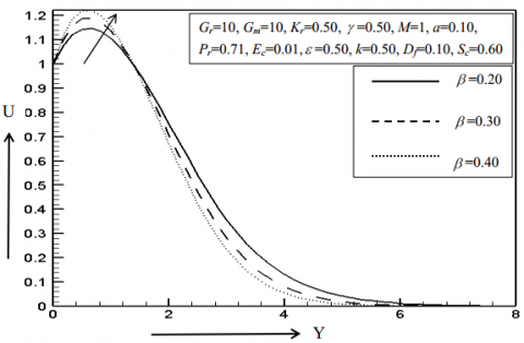
Figure 1. Impression of β on U
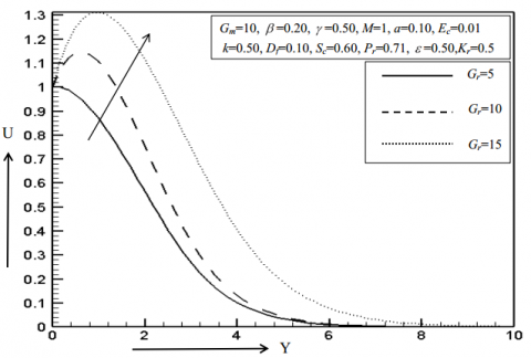
For graphical illustrations of the several flow profiles see the Figure 1 to Figure 10. We can see velocity distribution enhances for the enhance of Casson factor in Figure 1. We can also see the same result for thermal Grashof number in velocity profiles (Figure 2) because thermal buoyancy force gets enhance and the momentum boundary layer is progressing. The velocity curves boosts up 23.52% and 29.25% as it increases from 5 to 10 and 10 to 15.
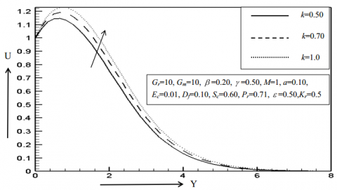
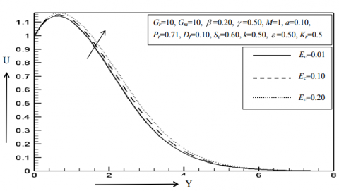
On the other hand, in Figure 3, it shows velocity outlines diminish with rise of magnetic factor because as the magnetic field intensity raises a resistive power is originated identified as Lorentz dynamism which inhibits the liquid stream thus velocity outlines decline. Here, the fluctuation of the curve declines 9.03% and 7.73% when the magnetic parameter progresses from 1 to 2 and 2 to 3 respectively. Figure 4 represents velocity profiles are developing for the rise of viscosity variation parameter. The increments of the boundary layers are 4.92% and 3.37% as the parameter changes from 0.5 to 1.5. The velocity distributions for permeability parameter and Eckert numeral are described in the Figure 5 and Figure 6. It is obvious from the graph that velocity sharply goes up due to rise in permeability parameter and Eckert number. In this case, 1.59% and 1.84% are the momentum boundary layers increment when Eckert number varies from 0.01 to 0.20 whilst the increments in the velocity curve are 5.87% and 4.80% for changing permeability parameter.
Figure 2. Impression of Gr on U
Figure 3. Impression of M on U
Figure 4. Impression of γ on U
Figure 5. Impression of k on U
Figure 6. Impression of Ec on U
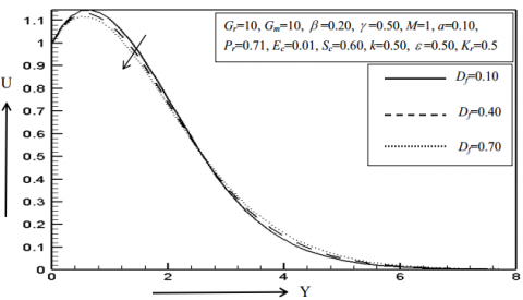
Figure 7. Impression of Df on U
Figure 8. Impression of ε on U
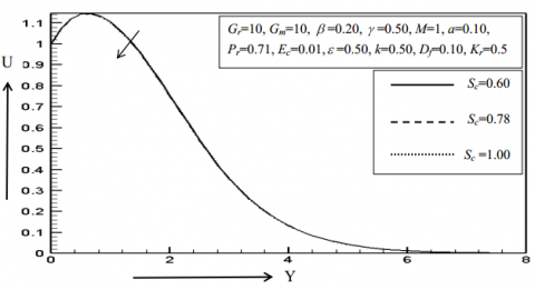
Figure 9. Impression of Sc on U
Figure 10. Impression of Kr on U
A reverse trend can be seen from Figure 7, it is evident that there is decrement of 2.21% and 1.85% because of increasing Dufour number whereas in Figure 8, velocity rises for boosting up the thermal conductivity parameter.
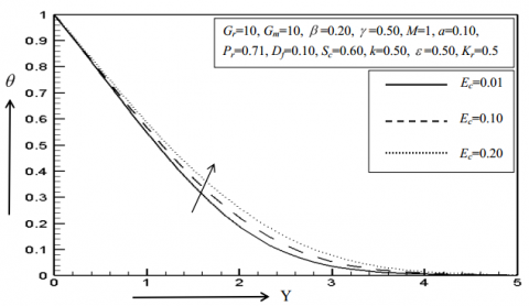
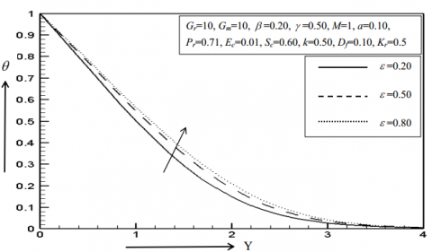
Figure 9 and Figure 10 inspect the impression of Schmidt factor and chemical reaction upon velocity field. Generally, the ratio of momentum and mass diffusivity is acquainted as Schmidt factor. It is identified that the momentum bounder phase drops because of rising appraise of Schmidt factor and chemical riposte generator. However, impacts of various factor on thermal boundary layers are displayed in the Figure 11 to Figure 13. As it is perceived from the delineate that warmth falls for raising the values of Dufour parameter in Figure 11 in which the boundary layer declines 2.99% and 2.58% for the increasing values of pertinent parameter. However, temperature goes up owing to the rise of Eckert factor and thermal conductivity parameter in Figure 12 and Figure 13. The energy gets enhance in the flow field due to the impact of viscous dissipation which yield a large buoyancy force such that the temperature rises up. On the other hand, the curve to curve fluctuation rises 4.59% and 1.76% in the thermal boundary layer as ε changes from 0.20 to 0.50 and 0.50 to 0.80.
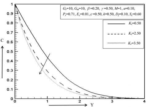
Figure 141 and Figure 115 discuss the coerce of Schmidt factor and chemical recompose parameter (destructive) on nano particle concentric profiles. Concentration rapidly drops for enhancing both the values of relevant parameters. At y= 1.0034, the numerical values obtained for Schmidt number and chemical reaction are 0.43706, 0.37559, 0.31582 and 0.43706, 0.28911, 0.24009 respectively. Thus we can see that chemical reaction parameter is diminishing the concentric profiles more significantly.
Figure 11. Impression of Df on θ
Figure 12. Impression of Ec on θ
Figure 13. Impression of ε on θ
Figure 14. Impression of Sc on C
Figure 15. Impression of Kr on C
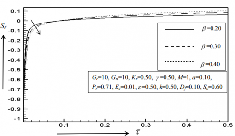
Figure 16. Impression of β on Sf
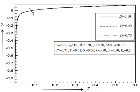
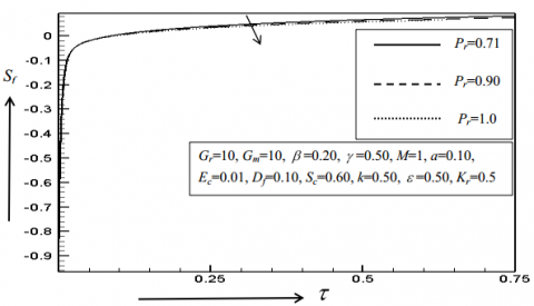
The skin factor and Nusselt factor are also demonstrated with assistance of graph. Skin friction is explained in the Figures 16, 17 and 18 for various values of Casson factor, Dufour generator and Prandtl producer. According to the figure, it is undeniable that skin friction goes down for raising the worth of these pertinent criterions. Elsewhere, Nusselt number reduces 0.23% and 0.17% for increasing value of thermal conductivity factor whilst the heat transference coefficient profile declines 0.48% and 0.53% for increasing values of Eckert number (Figure 19 and Figure 21).
However, the later one is diminishing the heat transfer coefficient profiles significantly. What is more, in Figure 20, it is clearly indicated that Nusselt factor profiles are progressing for the increment of Dufour number.
Figure 17. Impression of Df on Sf
Figure 18. Impression of Pr on Sf
Figure 19. Impression of ε on Nu
Figure 20. Impression of Df on Nu
Figure 21. Impression of Econ Nu
The mass and heat transfer behavior of viscous dissipative chemically reacted Casson fluid which is flowing with the impact of suction, thermal conductivity and variable viscosity is being discussed explicitly in this paper. The key outcomes are listed below.
|
B0 |
magnetic component, Wbm-2 |
|
$C^{\prime}$ $C_{w}^{\prime}$ |
nanoparticle concentration nanoparticle concentration at wall surface |
|
Df |
Dufour number |
|
Ec |
Eckert number |
|
Gr |
thermal Grashof number |
|
K Kr |
porous medium chemical reaction |
|
M |
magnetic parameter |
|
Nu |
local rate of heat transfer coefficient |
|
Pr |
Prandtl number |
|
R* |
reaction rate constant |
|
Sc |
Schmidt number |
|
Sf |
local skin friction coefficient |
|
$T^{\prime}$ $T_{w}^{\prime}$ |
fluid temperature, K temperature at wall surface, K |
|
$u^{\prime}, v^{\prime}$ |
velocity component in x, y direction, ms-1 |
|
Greek symbol |
|
|
b |
Casson fluid parameter |
|
b* |
concentration expansion coefficient |
|
κ |
thermal conductivity |
|
Κo |
coefficient of thermal conductivity constant |
|
$\vartheta$ |
kinematic viscosity, m2s-1 |
|
ρ |
density of the fluid, kg m-3 |
|
ε |
dimensionless thermal conductivity parameter |
|
γ |
dimensionless viscosity parameter |
|
Abbreviation |
|
|
MHD |
magnetohydrodynamics |
[1] Casson, N. (1959). A flow equation for pigment-oil suspensions of the printing ink type. In: Mill, C.C., Ed., Rheology of Disperse Systems, Pergamon Press, Oxford, 84-104.
[2] Rao, A.S., Prasad, V.R., Reddy, N.B., Beg, O.A. (2013). Heat transfer in a Casson rheological fluid from a semi-infinite vertical plate with partial slip. Heat Transfer Asian Research, 44(3): 272-291. https://doi.org/10.1002/htj.21115
[3] Bird, R.B., Dai, G.C., Yarusso, B.J. (1983). The rheology and flow of viscoelastic materials. Rev Chem Eng., 1(1): 1-83. https://doi.org/10.1515/revce-1983-0102
[4] Mitsoulis, E. (2007). Flows of viscoplastic materials: models and computations. The British Society of Rheology, 135-178.
[5] Mukhopadhyay, S. (2013). Casson fluid flow and heat transfer over a nonlinearly stretching surface. Chin Phys. B, 22(7): 074701. http://dx.doi.org/10.1088/1674-1056/22/7/074701
[6] Hayat, T., Shehzadi, S.A., Alsaedi, A. (2012). Soret and Dufour effects on magnetohydrodynamic (MHD) flow of Casson fluid. Appl Math Mech Engl. Ed., 33(10): 1301-1312. http://dx.doi.org/10.1007/s10483-012-1623-6
[7] Mustafa, M., Hayat, T., Pop, I., Aziz, A. (2011). Unsteady boundary layer flow of a Casson fluid due to an impulsively started moving flat plate. Heat Transfer, 40: 563-576. https://doi.org/10.1002/htj.20358
[8] Mishra, S.R., Baag, S., Mohapatra, D.K. (2016). Chemical reaction and soret effects on hydromagnetic micropolar fluid along a stretching sheet. Engineering Science and Technology, an International Journal, 19(4): 1919-1928. https://doi.org/10.1016/j.jestch.2016.07.016
[9] Kataria, H.R., Patel, H.R. (2016). Radiation and chemical reaction effects on MHD Casson fluid flow past an oscillating vertical plate embedded in porous medium. Alexandria Engineering Journal, 55(1): 583-595. https://doi.org/10.1016/j.aej.2016.01.019
[10] Animasaun, I.L. (2015). Effects of thermophoresis, variable viscosity and thermal conductivity on free convective heat and mass transfer of non-Darcian MHD dissipative Casson fluid flow with suction and nth order of chemical reaction. J Nigerian Math Society, 34(1): 11-31. https://doi.org/10.1016/j.jnnms.2014.10.008
[11] Animasaun, I.L., Oyem, A.O. (2014). Effect of variable viscosity, Dufour, Soret and thermal conductivity on free convective heat and mass transfer of non-Darcian flow past porous flat surface. American Journal of Computational Mathematics, 4(4): 357-365. http://dx.doi.org/10.4236/ajcm.2014.44030
[12] Pramanik, S. (2014). Casson fluid flow and heat transfer past an exponentially porous stretching surface in presence of thermal radiation. Ains Shams Eng. Journal, 5(1): 205-212. http://dx.doi.org/10.1016/j.asej.2013.05.003
[13] Arifuzzaman, S.M., Khan, M.S., Mehedi, M.F.U., Rana, B.M.J., Ahmmed, S.F. (2018). Chemically reactive and naturally convective high Speed MHD fluid flow through an oscillatory vertical porous plate with heat and radiation absorption effect. Engineering Science and Technology, an International Journal, 21(2): 215-228. https://doi.org/10.1016/j.jestch.2018.03.004
[14] Arifuzzaman, S.M., Biswas, P., Mehedi, M.F.U., Ahmmed, S.F., Khan, M.S. (2018). Analysis of unsteady boundary layer viscoelastic nanofluid flow through a vertical porous plate with thermal radiation and periodic magnetic field. Journal of Nanofluids, 7(6): 1122-1129. https://doi.org/10.1166/jon.2018.1547
[15] Arifuzzaman, S.M., Khan, M.S., Mamun, A.A., Reza-E-Rabbi, S.K., Biswas, P., Karim, I. (2019). Hydrodynamic stability and heat and mass transfer flow analysis of MHD radiative fourth-grade fluid through porous plate. Journal of King Saud University-Science, 301(4): 1388-1398. https://doi.org/10.1016/j.jksus.2018.12.009
[16] Hayat, T., Shah, E., Alsaedi, A., Hussain, Z. (2017). Outcome of homogenous and heterogeneous reactions in Darcy-Forchheimer flow with nonlinear thermal radiation and convective condition. Results in Physics, 7: 2497-2505. http://dx.doi.org/10.1016/j.rinp.2017.06.045
[17] Xuan, Y., Roetzel, W. (2000). Conceptions for heat transfer correlation of nanofluids. International Journal of Heat and Mass Transfer, 43(19): 3701-3707. https://doi.org/10.1016/S0017-9310(99)00369-5
[18] Azam, M., Khan, M., Alshomrani, A.S. (2017). Effects of magnetic field and partial slip on unsteady axisymmetric flow of Carreau nanofluid over a radially stretching surface. Results in Physics, 7: 2671-2682. http://dx.doi.org/10.1016/j.rinp.2017.07.025
[19] Khanafer, K., Kambiz, V., Marilyn, L. (2003). Buoyancy-driven heat transfer enhancement in a two-dimensional enclose utilizing nanofluids. International Journal of Heat and Mass Transfer, 46(19): 3639-3653. http://dx.doi.org/10.1016/s0017-9310(03)00156-x
[20] Mamatha, U.S., Raju, C.S.K., Mahesha, Saleem, S. (2018). Nonlinear unsteady convection on micro and nanofluids with Cattaneo-Christov heat flux. Results in Physics, 9: 779-786. http://dx.doi.org/10.1016/j.rinp.2018.03.036
[21] Sulochana, C., Ashinkumar, G.P., Sandeep, N. (2016). Transpiration effect on stagnation-point flow of Carreau nanofluid in the presence of thermophoresis and Brownian motion. Alexandria Engineering Journal, 55(2): 1151-1157. http://dx.doi.org/10.1016/j.aej.2016.03.031
[22] Khan, M., Malik, M.Y., Salahuddin, T., Arif, H. (2018). Heat and mass transfer of Williamson nanofluid flow yield by an inclined Lorentz force over a nonlinear stretching sheet. Results in Physics, 8: 862-868. http://dx.doi.org/10.1016/j.rinp.2018.01.005