Yuva Krishna Aluri![]() | Vandavagula Satya Anusuya Devi
| Vandavagula Satya Anusuya Devi![]() | Manjunath Chinthakunta
| Manjunath Chinthakunta![]() | Manohar Manur
| Manohar Manur![]() | Praveen Kumar Jayapal
| Praveen Kumar Jayapal![]() | Gunapriya Balan
| Gunapriya Balan![]() | Kranthi Kumar Lella*
| Kranthi Kumar Lella*![]()
© 2024 The authors. This article is published by IIETA and is licensed under the CC BY 4.0 license (http://creativecommons.org/licenses/by/4.0/).
OPEN ACCESS
A crucial natural resource that directly affects the ecology is forests. Forest fires have become a noteworthy problem recently as a result of both natural and man-made climatic changes. A smart city application that uses a forest fire discovery technology based on artificial intelligence is provided in order to prevent significant catastrophes. A major danger to the environment, animals, and human lives is posed by forest fires. The early detection and suppression of these fires is crucial. This work offers a thorough method for detecting forest fires using advanced deep learning (DL) algorithms. Preprocessing the forest fire dataset is the initial step in order to improve its relevance and quality. Then, to enable the model to capture the dynamic character of forest fire data, long short-term memory (LSTM) networks are used to extract useful feature from the dataset. In this work, weight optimisation in LSTM is performed using a Modified Firefly Algorithm (MFFA), which enhances the model's performance and convergence. The Variational Autoencoder Generative Adversarial Networks (VAEGAN) model is used to classify the retrieved features. Furthermore, every DL model's success depends heavily on hyperparameter optimisation. The hyperparameters of an VAEGAN model are tuned in this research using the Waterwheel Plant Optimisation Algorithm (WWPA), an optimisation technique inspired by nature. WPPA uses the idea of plant growth to properly tune the VAEGAN's parameters, assuring the network's peak fire detection performance. The outstanding accuracy (ACC) of 97.8%, precision (PR) of 97.7%, recall (RC) of 96.26%, F1-score (F1) of 97.3%, and specificity (SPEC) of 97.5% of the suggested model beats all other existing models, which is probably owing to its improved architecture and training techniques.
forest fire, long short term memory, modified firefly algorithm, waterwheel plant optimization, variational autoencoder
Forests are crucial to maintaining our way of life because they provide a wealth of priceless resources, such as minerals and materials required for several industrial operations [1]. Beyond their obvious benefits, trees considerably improve the environment by purifying the air naturally, collecting carbon dioxide, and releasing oxygen that sustains life. Additionally, trees provide crucial habitat for a variety of species and act as a barrier against sandstorms, safeguarding crops besides maintaining ecological balance. But the widespread effects of climate change [2, 3] are mostly to blame for the increasing frequency of forest fires in recent years. High temperatures and dry circumstances encourage the spread of flames, causing significant damage to ecosystems, animal habitats, natural reserves, and a clear danger to people's lives. Notably, coniferous woods, which are distinguished by their needle- or cone-shaped foliage, are especially vulnerable to fires because the sap found in their branches is flammable [4]. Coniferous trees' dense growth patterns also contribute to the fast-moving spread of flames. Millions of acres of forest are annually destroyed as a result of this worrying trend, with catastrophic economic consequences.
Many nations, including the fires. In particular, the horrific Australian bushfires in 2020 provide as a sobering example of the intensity of these occurrences, resulting in the irreparable loss of forest resources, innumerable animal deaths, and human casualties. These flames destroyed 1,500 dwellings, approximately 500,000 animals, about 14 million acres of forest, and nearly a third of all living things [5]. Similarly, in 2018 and 2019, devastating wildfires of equal size burned large areas of the Amazon rainforest and California's forests, causing enormous losses [6]. Surprisingly, between 1992 and 2015, human activity was responsible for a whopping 85% of forest fires in the United States, with natural causes like lightning strikes and the effects of climate change accounting for the remaining 15%. More stringent regulations and reasonable practises may have prevented many of the human-caused fires [7]. It is noteworthy to note that during the worldwide COVID-19 epidemic, the frequency of forest fires decreased as several nations instituted lockdown measures that restricted human activity, hence decreasing the risk of human-induced fires [8].
DL networks have been a very successful method for addressing the crucial problem of forest fire detection. DL has shown its aptitude in a number of fields, including autonomous machine translation [9] and image and video categorization. This was made possible by DL's capacity to automatically extract and categorise properties from data stored on the same network [10]. DL is especially good at detecting forest fires because to large datasets and improved processing capacity. For both ground-based and aerial images, DL-based systems have shown their superior performance over conventional machine learning techniques in handling the complexity of forest fire categorization and detection [11, 12]. The rise of automated DL fire detection systems holds enormous potential for the development of AI fire models are a useful tool for addressing this pressing environmental issue since they can quickly and precisely identify and track flames inside the camera's field of vision [13].
In subsequent work, we intend to look into the following possible improvements:
Attention Mechanisms: By including attention mechanisms in the LSTM architecture, the model may be better able to identify significant patterns in the data by focusing on pertinent elements at certain time steps.
Ensemble approaches: By integrating several LSTM models or other recurrent neural network (RNN) types, one can improve the model's prediction presentation and robustness by using ensemble approaches.
Hybrid Architectures: Investigating hybrid architectures that integrate transformer models or convolutional neural networks (CNNs) with LSTM may offer supplementary benefits in sequence modelling and feature extraction.
This paper's primary contributions are:
-The dataset for this investigation was first pre-processed. This research then improves the quality of information related to forest fires by using cutting-edge DL methods and extracts useful temporal characteristics using LSTM networks.
-The performance and convergence of the LSTM model are improved by the application of the MFFA for weight optimisation.
-As a tool for classification, the VAEGAN model is used. The WWPA for hyperparameter tuning promises to greatly improve the ACC and efficacy of systems for detecting forest fires. Results are analyzed using five parameter metrics.
The rest of the research is structured like shadows: The literature review is presented in Section 2, followed by a brief explanation of the proposed model in Section 3, the results and validation analysis in Section 4, and finally, a conclusion and summary are given in Section 5.
Abdusalomov et al. [14] developed a better strategy for spotting forest fires, according to their study. The Detectron2 platform, an enhanced version that was constructed from the ground up utilising DL techniques to replace the original Detectron library, is the foundation of their strategy. To help in the training of their model, they carefully chose and annotated a special dataset; this critical step ultimately resulted in a model with more ACC than rival methods. A dataset of 5200 photographs served as the testing ground for the researchers as they modified the Detectron2 model under various situations. Notably, their model proved the ability to recognise even little fires at large distances, day or night. Their method's usage of the Detectron2 algorithm, which enables long-range detection, has several advantages. Their investigations' real findings supported the ACC of their method for spotting forest fires. They were able to identify forest fires with a stunning ACC rate of 99.3%, proving the reliability and power of their recommended technique.
The GXLD technique, developed by Huang et al. [15], combines a defogging algorithm with a lightweight YOLOX-L model to identify forest fires. The dark channel prior approach is used by GXLD to remove fog from photos, producing sharper, fog-free images. On top of that, they improved the YOLOX-L model by adding elements from SENet, GhostNet, and depth separable convolution, resulting in YOLOX-L-Light. Then, using the defogged photos, this optimised model is used to identify forest fires. The researchers used the mean average Pr (mAP) metric to rate detection ACC and network parameters to determine the model's lightweightness in order to evaluate the performance of YOLOX-L-Light and GXLD. They ran trials on their dataset of forest fires, and the results showed a considerable improvement. YOLOX-L-Light increased the mAP by 1.96% while reducing the model's parameters by 92.6%. Notably, GXLD outperformed YOLOX-L by 2.46% with a remarkable mAP of 87.47%. Furthermore, GXLD provided an average frame rate of 26.33 frames per second when set up with an input picture size of 1280 720. Amazingly, GXLD displayed real-time forest fire detection skills with great ACC, strong target confidence, and sustained target integrity even under difficult foggy circumstances.
Chen et al. [16] introduced the YOLOv5s-CCAB, an improved variant of the YOLOv5s architecture for multi-scale forest fire detection, in their article. This model has seen a number of revisions. They initially introduced Coordinate Attention (CA) to YOLOv5s to direct the network's focus especially on traits associated with forest fires. Second, they developed a CoT3 module to improve the identification of forest fires, reduce parameter complexity, and have the capacity to capture global dependencies in photographs of forest fires. In order to raise the network's PR while detecting potential forest fire targets, the Complete-Intersection-Over-Union (CIoU) Loss function was enhanced. A Bi-directional Feature Pyramid Network (BiFPN) was constructed within the model's neck to increase its ability to correctly fuse the extracted forest fire features. According to the testing outcomes and their specially developed multi-scale forest fire dataset, YOLOv5s-CCAB resulted in significant improvements. It retains the high Frames Per Second (FPS) rate of 36.6 and reaches a rate of 87.7% for the AP@0.5 metric, a startling 6.2% increase. These results demonstrate the model's very fast and accurate identification. In light of this, YOLOv5s-CCAB provides an advantageous point of reference for applications requiring precise, real-time multi-scale forest fire detection.
For their study, Zhang et al. [17] created the multi-scale feature extraction model (MS-FRCNN) for the detection of small target forest fires. This model enhances the conventional Faster RCNN detection technique. Instead of VGG-16, ResNet50 was employed as the backbone network to lessen the possibility of gradient dispersion or explosion during feature extraction. In order to benefit from multi-scale feature extraction, they also integrated a Feature Pyramid Network (FPN), which increased the MS-FRCNN's ability to capture comprehensive feature data. They also included a brand-new attention module called PAM to help the Regional Proposal Network (RPN) focus more on the semantic and geographic details of small target forest fires and decrease the distraction from complex backgrounds. The model also substituted the soft-NMS algorithm for the traditional NMS technique in order to reduce errors in identified frames. They conducted trials using their carefully curated multi-scale forest fire dataset, and the findings revealed a substantial 5.7% increase in detection ACC above baseline models. This shows how the multi-scale feature extraction approach forest fires.
A technique for recognising forest fires was proposed by Rahman et al. [18] using a Convolutional Neural Network (CNN) architecture and freshly created fire detection dataset from another study. Their approach utilised separable convolution layers for rapid fire detection, making it suitable for real-time applications. After training on their dataset, the method showed a remarkable 97.63% ACC in identifying forest fires in photos, along with a 98.00% F1 and an 80% Kappa value. These results show the method's potential to be a helpful tool for early fire breakout identification, enabling authorities to act promptly and put preventive measures in place to minimise damage.
A system for early fire detection and classification was constructed by Avazov et al. [19] using the Internet of Things (IoT) and YOLOv5. They use IoT devices in their investigation to verify if fires that YOLOv5 claimed to have seen may have been fabricated or unreported. The successful findings shown that IoT may be used to monitor and verify fire incidents in real-time. This approach may greatly improve its capacity to reduce forest fires. A system architecture for autonomous forest fire detection utilising DL image processing methods was suggested in a paper by Ye et al. [20], and it was especially created for tiny UAV applications. The optimisation process included a number of phases, including switching to ShuffleNetV2 as the backbone network, pruning the network, sparse training, tuning, and hardware acceleration. According to experimental findings, their forest fire detection system increased inference speed by 50%, decreased CPU utilisation and temperature by 35% and 25%, and consumed 10% less power while retaining an ACC of 92.5%. It's noteworthy that the model's ACC remained steady despite alterations in the bird's-eye view angle.
As an alternative to more traditional models like Fast R-CNN and Faster R-CNN, Al-Smadi et al. [21] investigated the efficacy of a framework intended to reduce the sensitivity of a number of YOLO detection methods. On a multi-oriented dataset for recognising forest smoke, they employed YOLOv5x to increase their model's mean average Pr (mAP) ACC from earlier gold-standard techniques to an astounding 96.8%. Additionally, YOLOv7 outperformed YOLOv3 with a 95% mAP ACC. These findings supported the method's outstanding ability to find forest fires in spite of challenging environmental conditions.
Talaat and ZainEldin [22] presented the discovery system (SFDS), based on the YOLOv8 algorithm, as an enhanced fire detection method for smart cities. This system employed DL to distinguish fire-specific traits in real-time, potentially improving fire detection ACC, reducing false alarms, and offering a more cost-effective alternative to traditional methods. The application, fog, cloud, and IoT layers of the recommended architecture employed cloud and fog computing to acquire and analyse data in real-time. The SFDS achieved a high success rate of 97.1% for all classes and is useful for various applications, such as fire safety management and intelligent security systems in smart cities.
Although these existing models for detecting forest fires have showed potential, they still have issues with Pr, dependability, and flexibility. Our model offers numerous significant advances in an effort to reduce the harmful impacts of forest fires and enhance early detection.
We will discuss the compatibility of the proposed model with existing forest fire prevention and control systems, ensuring that it can seamlessly integrate into the current infrastructure without requiring significant modifications. Compatibility considerations may include data formats, communication protocols, and system architectures.
We will highlight the model's potential to serve as a real-time decision support tool for forest fire prevention and control. By continuously analyzing incoming data from various sources such as remote sensors, weather positions, and satellite imagery, the model can provide early warnings, identify high-risk areas, and assist in resource allocation and deployment strategies. Figure 1 shows the flow of the suggested model.
Figure 1. Work flow of the proposed model
3.1 Dataset description
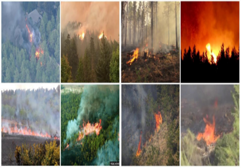
As exposed in Figure 2, the dataset utilised in this study consists of 3000 images of forest fires that were captured by drones and video surveillance equipment in various forest environments. It also includes additional forest fire datasets discovered using web crawling techniques and publicly available forest fire datasets [23]. This collection's 1000 images all have hand annotations. Then, these 1000 annotated images were divided into two subsets: 300 served as a specialist test set to assess the model's ACC, and 700 were set aside for training purposes to construct a prototype forest fire detection model. 2000 images of unlabelled forest fires were also included in the dataset and utilised in the training process.
Figure 2. Schematic diagram of forest fire data set
3.2 Preprocessing
The dataset provides a wide range of photos taken from different perspectives, enabling the algorithm to identify between forest fire and non-fire events with greater ACC. With the help of this information, the model is equipped to recognise forest fires based on two key criteria: the existence of fire flames and the presence of fire flames mixed with smoke. Up to this point, our main attention has been on the exacting standards used to divide up the dataset into an equal number of images with fire (1) and those without fire (0) [24]:
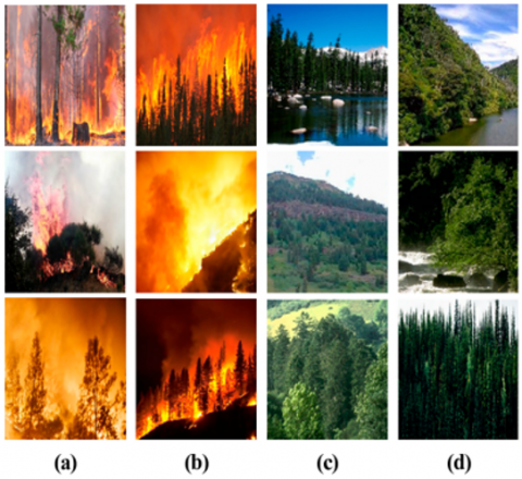
Fire (1): Images of forests and mountain ranges that are enveloped in flames and/or smoke brought on by fires.
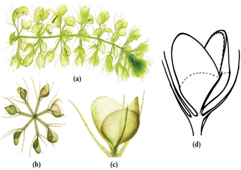
Figure 3. Images from (a) and (b) Fire class and (c) and (d) No-Fire class
No-Fire (0): Consisting of a wide variety of pictures showing forest and mountain vistas devoid of fire. This categorization method was developed to make it easier to train models with a variety of images while avoiding misunderstanding with situations that could seem similar, such mountain sunsets.
The goal of this meticulous dataset refining method was to improve overall model performance and streamline the model training procedure. As they were the most contextually relevant to our study objective at this dataset curation phase, we particularly cropped pictures of fires in mountainous or forest settings. After then, every image was scaled consistently such that it had the same size, 250×250 pixels. These preprocessing methods were crucial in helping the model successfully include important information about forest fires. Figure 3 shows visual representations of both the fire and no-fire categories within forest fire dataset.
3.3 LSTM feature extraction
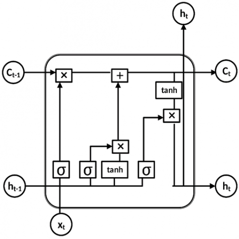
After the preprocessing phase, the input characteristics are then passed to the LSTM module, a crucial component of our methodology [25]. Due to the huge quantity of data gathered from the dataset, a typical RNN would not be sufficient for our purposes. Gradient disappearance and explosion issues are addressed via a customised RNN iteration known as LSTM. During the training phase, RNN creates temporal connections between prior states and the inputs to provide predictions. RNN, on the other hand, finds it challenging to maintain the past because to its limited memory capacity, especially when dealing with massive volumes of time series data. However, LSTM excels at classifying enormous time series datasets and locating temporal correlations. Its use covers several sectors and yields outstanding results for tasks like speech recognition and image classification.
The LSTM architecture seen in Figure 4 has special memory cells designed to make use of prior knowledge and maintain key characteristics from massive volumes of time series data. These memory cells may store and apply the information that was learnt, allowing the model to process and classify input effectively.
Figure 4. Architecture of LSTM
The output gate, also known as the ot gate, the forget gate, also known as the ft gate, and the input gate all play distinct roles in regulating information flow in the LSTM architecture.
The major responsibility of the forget gate is to decide what data to preserve and what to discard within the cell state. It does this by conducting a pointwise multiplication operation using the inputs $x_t$, the current input, and $h_{t-1}$, the previous hidden state information. By using the sigmoid activation function, the forget gate generates an output that is either 0 or 1. Keeping important information in the cell state is indicated by a value of 1 , whilst removing unimportant information is indicated by a value of 0 . The forget gate, input gate, and output gate's core characteristics are explained in literature [26] by Eq. (1) to Eq. (6).
$f_t=\sigma\left(W_f\left[h_{t-1}, x_t\right]\right)+b_f$ (1)
The forget gate, or $f_t$, is subjected to a bias called $b_f$, and the process weight $W_f$ stands for that. The forget gate is activated using the activation function, represented by the letter "s," to allow choice. Next, a critical decision on whether data should be kept in the cell state, $C_t$, must be made by the input gate. It considers both the input, $x_t$, and the preceding hidden state, $h_{t-1}$ to arrive at this conclusion. Eq. (2) and Eq. (3) describe the pointwise multiplication of the forget gate, $f_t$, and hyperbolic tangent (tanh) activation functions in this decision-making process:
$i_t=\sigma\left(W_i\left[h_{t-1}, x_t\right]\right)+b_i$ (2)
$C_t=\tan h\left(W_c\left[h_{t-1}, x_t\right]\right)+b_0$ (3)
While $b_i$ and $b_c$ stand for the biases of the neural network, $W_i$ and $W_c$ stand for the weights connected to the input gate $\left(i_t\right)$ and output gate $\left(o_t\right)$. The information about the previous concealed cell state is denoted by the word $C_t$. Eq. (4) shows how we combine Eq. (2) and Eq. (3) to conduct a pointwise addition operation in order to update the current cell state, $C_t^{\prime}$:
$C_t^{\prime}=\left(f_t \times\left(C_t\right)\right)+\left(i_t \times\left(C_t\right)\right)$ (4)
The output gate is calculated in Eq. (5). The current input, represented as $x_t$, and the prior hidden state, $h_{t-1}$, which incorporates the activation function $s$, are both used in this gate. In order to further hone the output network, a bias term called $b_0$ is included.
$o_t=\sigma\left(W_o\left[h_{t-1}, x_t\right]\right)+b_o$ (5)
A pointwise multiplication operation is used to combine the information from the cell state, $C_t$, with the updated output gate, indicated as $o_t$. The hidden state that follows, $h_t$, is produced by this procedure and is represented in Eq. (6).
$h_t=\sigma\left(O_t \times \tan h\left(C_t^{\prime}\right)\right)$ (6)
The LSTM model may be improved significantly by using optimal parameters. The efficacy of feature extraction is substantially influenced by these characteristics. With the exception of the completely linked dense layer, 50 more neurons have been added to each layer to aid in better training. Furthermore, a 20% dropout rate has been used to allay any overfitting concerns.
3.3.1 Weight optimization in LSTM using MFFA
Firefly algorithm. In situations where it is necessary to optimise not one, but several competing objectives at once, WWPA can handle these difficulties. By efficiently exploring the trade-off between different objectives, WWPA can discover Pareto-optimal solutions that represent the best compromise between competing goals.
Efficient exploration and exploitation. WWPA balances exploration (searching diverse regions of the hyperparameter space) and exploitation (exploiting promising 0refine solutions) effectively. This balanced exploration-exploitation trade-off enables WWPA to quickly converge to high-quality solutions while avoiding premature convergence to suboptimal regions.
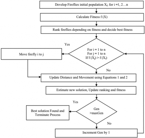
Figure 5. Flowchart of modified firefly algorithm
The Firefly Algorithm, a metaheuristic method that was motivated by the flashing behaviour of fireflies. This tactic is based on the idea that different fireflies have different levels of attraction and that this impacts how they mate [27, 28].
The modified firefly algorithm [29-31] improves on the original Firefly Algorithm by reducing its inherent volatility and improving firefly movement. Figure 5 depicts the Modified Firefly Algorithm's flowchart and the sequential steps it goes through. The Modified Firefly Algorithm's randomization parameter $\alpha$ represents the start and finish values for each iteration as $\alpha_0$ and $\alpha_{\infty}$, respectively. Higher values of this strategy $\alpha$ lead to better convergence while attempting to strike a balance between the capabilities of exploitation and exploration. The ith lightning bug motion and the distance function $r_i$ are described in Eq. (7) and Eq. (8), respectively.
$r_{i,{ best }}=\left(x_i-x_{{gbest }}\right)^2+\left(y_i-y_{{gbest }}\right)^2$ (7)
$x i=x i+\beta_0 e^{-\gamma t^2 y}(x j-x i)+\beta_0 e^{-\gamma t^2} t$, best $\left(X_{{gbest }}-X_i\right)+\alpha \varepsilon+\lambda \varepsilon\left(x_i-g b e s t\right)$ (8)
where, $\varepsilon= rand-1 / 2, gbest = global best$. When a local best solution is not available close by, the ith firefly is drawn to the best choice. The MFFA reduces the possibility of becoming stranded in local optima by carefully limiting unpredictability. Fireflies may progress towards the global optimum thanks to the rapid convergence brought on by this well controlled randomness reduction. Please refer to Figure 5 for a flowchart illustrating the Modified Firefly Algorithm's steps and sequence.
3.4 VAEGAN classification
In this work, the classification of data related to forest fires is done using VAEGAN. during GAN (Generative Adversarial Network) excels at creating samples precisely, it often exhibits instability during learning. Contrarily, VAE (Variational Autoencoder) generates a variety of samples while retaining a respectable amount of stability during the course of learning. The VAEGAN framework may take use of the advantages that each of these generative models have to offer by combining them. VAEGAN is able to deliver samples that are both highly fidelity and variety while keeping their stability while learning is taking place. Typically, an encoder plus a decoder makes up a VAE [32]. The input data must be transformed into a latent vector by the encoder, and the decoder must estimate the input from the latent vector. The mathematical representations of the encoder and decoder processes are shown in Eq. (9) and Eq. (10), respectively.
$z \sim \operatorname{Enc}(x)=q_\phi(z \mid x)$ (9)
$\hat{x} \sim \operatorname{Dec}(z)=p_\phi(x \mid z)$ (10)
In this situation, the input, latent vector, and estimated input are each represented by $\mathrm{x}, \mathrm{z}$, and $\hat{x}$. The encoder and decoder models are affected by the parameters $\phi$ and $\theta$. The genuine posterior $p_\phi(x \mid z)$ is approximated by the term $q_\phi(z \mid x)$. The reconstruction error and a previous regularisation term, which are added together, make up the two halves of the loss function connected to VAE.
$J_{V A E}=J_{\text {recon }}+J_{\text {prior }}$ (11)
$J_{\text {recon }}=-E_{q \phi(z \mid x)}\left[\log p_\theta(x \mid z)\right]$ (12)
$\hat{x} \sim \operatorname{Dec}(z)=p_\phi(x \mid z)$ (13)
where, $D_{K L}$ and $p_\phi(z)$ represent the prior distribution of $\mathrm{z}$ and the Kullback-Leibler divergence. A GAN model's generator and discriminator are its usual components [32]. Probability $a$ and probability $1-a$ are assigned by the discriminator, whereas the generator translates the latent vector to data space. The primary goal of a GAN is to discover a discriminator that can differentiate between generated and real data, while also adjusting the generator to fit the distribution of real data. As a function of both the discriminator and generator, the binary cross entropy represents the loss function of a GAN.
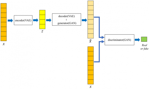
Figure 6. Structure of VAE-GAN
$v=Dis(u) \epsilon[0,1], u=Gen(w)$ (14)
$J_{G A N}=\log ({Dis}(u))+\log (1-{Dis}({Gen}(w)))$ (15)
In this instance, "w" is a random variable represented by the probability density function p(w), and "u" represents a genuine sample. While it's true that GANs may produce synthetic data without using density functions in certain circumstances, such as when dealing with unbalanced data, there are other situations when getting fresh samples from the generator with specified distributions might be advantageous. In order to do this, a generative model is built by using the VAE's decoder component as the GAN's generator. A visual illustration of the VAE-GAN model's structure is shown in Figure 6.
The following is a representation of the loss function of the VAE-GAN [32].
$J_{V A E-G A N}=J_{\text {prior }}+J_{D i s_l}+J_{G A N}$ (16)
$J_{D i s_l}=-E_{q(Z \mid x)}\left[\log p\left(D i s_l(x) \mid z\right)\right]$ (17)
where, $\operatorname{Dis}_l(x)$ denotes a Gaussian observation model with an identical covariance and $D i s_l(\tilde{x})$ as the mean.
3.4.1 Hyper parameter tuning using WWPA
The WWPA is described in this section. Here, we explore the motivation behind the method and provide a thorough mathematical explanation of how it works.
Figure 7. Image of the WW plant. (a) A side view of a shot that is free-floating and loaded with traps. (b) Frontal view with both open and shut traps. (c) Just one open trap. (d) An open trap schematic illustration
Inspiration of WWPA. Aldrovanda vesiculosa, the alternative name for the waterwheel (WW) plant, has broad petioles that contain its unusual traps, which are barely 1/12 inches in size and resemble tiny transparent flytraps [33]. The interactions with other aquatic plants won't cause these traps to deteriorate or unintentionally activate because of their skilled design. They are protected by a ring of bristles that resemble hair. These traps include a variety of hook-like teeth along their edges that interlock when the trap catches its victim, much like the teeth seen in a typical flytrap. The Aldrovanda trap has more than 40 elongated trigger hairs, compared to the normal 6-8 trigger hairs on a Venus flytrap. When one or more triggers are pulled, these trigger hairs allow the trap to shut. These carnivorous plants have trigger hairs as well as glands that emit acid to help in the digesting of their caught prey. The sealant and the plant's interlocking teeth trap the prey. By leading the prey towards the hinge at the base of the trap, the seal successfully catches the prey. The body fluids of the prey are extensively broken down by the plant's digestive secretions, and any leftover material is excreted. Similar to a flytrap, an Aldrovanda trap can hold and digest two to before filling to capacity. The infrastructure of the waterwheel plant is shown in Figure 7.
The WWPA mathematical model. This section describes how WWPA is set up before going into detail about how the WW's location is updated throughout both the exploration and exploitation phases using a classical based on the actual behaviour of WWs.
Initialization. The population-based approach of the WWPA tries to locate the ideal solution by using the collective search capabilities of its population members within the solution space. Each of the WWs that make up the population of this algorithm represents a potential resolution to the problem and has a specific set of problem-related variables. Vectors may be used to formally represent these responses. The whole population of the WWPA, which consists of all WWs as given in Eq. (18), may be represented by a matrix. At the beginning of WWPA, the positions of these WWs inside the solution space are initialised at random using Eq. (19).
$P=\left[\begin{array}{c}P_1 \\ \vdots \\ P_i \\ \vdots \\ P_N\end{array}\right]=\left[\begin{array}{ccccc}p_{1,1} & \cdots & p_{1, j} &\cdots & p_{1, m} \\ \vdots & \ddots & \vdots & \ddots & \vdots \\ p_{i, 1} & \cdots & p_{1, j} & \cdots & p_{i, m} \\ \vdots & \ddots & \vdots & \ddots & \vdots \\ p_{N, 1} & \cdots & P_{N, j} & \cdots & P_{N, M}\end{array}\right]$ (18)
$\begin{aligned} & p_{i, j}=l b_j+r_{i, j .}\left(u b_j-l b_j\right) \\ & i=1,2, \ldots, N, j=1,2, \ldots, m\end{aligned}$ (19)
where, $\mathrm{N}$ stands for the quantity of WWs, and $\mathrm{m}$ stands for the quantity of variables. The limits for the $\mathrm{j}$-th issue variable are represented by $l b_j$ and $u b_j$, while the variable $r_{i, j}$. has random values between $[0,1]$. The population matrix of WW locations is designated as $\mathrm{P}$, where $p_i$ is the $\mathrm{j}$-th $\mathrm{WW}$, which corresponds to a problem variable, and $p_{i, j}$ denotes its i-th dimension. The target function may be calculated for each WW as they each stand in for a possible answer to the issue. Studies have proven that a vector may be used to properly represent the variables that make up the objective function in Eq. (20).
$F=\left[\begin{array}{c}F_1 \\ \vdots \\ F_i \\ \vdots \\ F_N\end{array}\right]=\left[\begin{array}{c}F\left(X_1\right) \\ \vdots \\ F\left(X_i\right) \\ \vdots \\ F\left(X_N\right)\end{array}\right]$ (20)
where, F denotes the vector containing all of the values for the objective functions, and $F_i$ is the i-th WW. Most of the time, objective are used to choose the best keys. The best candidate solution, indicated by the highest objective function value, and the worst candidate solution, indicated by the lowest value, are thus the most crucial metrics. Given that WWs pass across the search region at varying speeds throughout each iteration, the optimal solution could evolve over time.
Stage 1: Recognising positions and hunting for insects
WWs flourish as skilled hunters capable of locating pests because to their exceptional sense of smell. A WW attacks as soon as it notices an insect nearby, focusing on the bug's particular location and starting a chase to trap it. For the first stage of its populace update procedure, the WWPA simulates the behaviour of a WW. The WWPA improves its exploration skills by modelling the hunting behaviours of WWs, allowing it to find ideal places while avoiding being caught in local optima. This is accomplished by simulating the large motions of the WW as it approaches the insect within the solution space. This simulation of the WW's approach to the insect is integrated using an Eq. (21) as shown below, to predict the WW's new location. If moving the WW to the newly determined position increases the charge of the target function, as shown in Eq. (21) and Eq. (22), the old position is abandoned in favour of the new one.
$\vec{W}=\vec{r}_{1 .}(\vec{P}(t)+2 K)$ (21)
$\vec{P}(t+1)=\vec{P}(t)+\vec{W} .\left(2 K+\vec{r}_2\right)$ (22)
Alternately, the WW's location may be changed using the following Eq. (23) if the results do not improve after three consecutive repetitions:
$\vec{P}(t+1)=\operatorname{Gaussian}\left(\mu_p, \sigma\right)+\vec{r}_1\left(\frac{\vec{P}(t)+2 K}{\vec{W}}\right)$ (23)
In this Eq. (23) the random variables $\vec{r}_1$ and $\vec{r}_2$ may, respectively, have values of 0 or 2 and 0 or 1 . The vector $\vec{W}$ represents the radius of each circle that the WW plant evaluates as possible regions, and $\mathrm{K}$ is a variable with values between 0 and 1 .
Stage 2: Carrying the insect in the suitable tube (exploitation)
The behaviour of insects being transported to feeding tubes by waterwheels serves as the model for the second stage of population updates in WWPA. By simulating this behaviour, WWPA may improve its convergence towards answers that are very similar to those it has already collected. WWPA modifies the location of the WW inside the problem region by simulating the insect's journey to the proper tube for ingestion. To do this, each WW was first placed in a fresh, arbitrary position that represented a "favourable region for insect consumption," according to the WWPA designers. Eq. (24) and Eq. (25) show that if the objective function produces a better value at the new position, the WW is moved.
$\vec{W}=\vec{r}_3\left(K \vec{P}_{\text {best }}(t)+r_3 \vec{P}(t)\right)$ (24)
$\vec{P}(t+1)=\vec{P}(t)+K \vec{W}$ (25)
After three iterations, if the response still doesn't indicate progress, the method incorporates a mutation process akin to the exploration stage. The algorithm undergoes certain alterations throughout this mutation phase to avoid being stuck in local minima. In this adaptive method, the current answer, indicated as $\vec{P}$ at iteration $t$, is represented as $(\mathrm{P})$ at iteration $\mathrm{t}$, and the ideal solution is written as $\vec{P}_{\text {best }}$. A random mutable with values between $[0,2]$ is $\vec{r}_3$. This strategy aids the algorithm's robustness and effective escape from local maxima.
$\vec{P}(t+1)=\left(\vec{r}_1+K\right) \sin \left(\frac{F}{C} \theta\right)$ (26)
where, [-5, 5] is a range for the random variables F and C's values. Additionally, using the Eq. (27), K's value falls down rapidly.
$K=\left(1+\frac{2 * t^2}{T_{\max }}+F\right)$ (27)
The proposed WWPA's pseudocode
The iterative process used by the WWPA has the following three phases. Once the first and second steps are complete, each WW is moved in the third and final stage. This adjustment, which results in the key adjustments of the best candidate solution, is based on a comparison of target function values. The WW positions are then adjusted in preparation for the next iteration. This repeated process is carried out till the algorithm achieves its conclusion. Implement WWPA as instructed, following the detailed instructions in Algorithm 1. Based on its iterative development, WWPA offers the most promising candidate solution after being completely deployed.
|
Algorithm 1: The projected algorithm of WWPA |
|
1: Place the WW plants' initial placements $P_i(i=1,2, \ldots, n)$ for n function $f_n$, iterations $T_{\max }$, parameters of $r, \vec{r}_1, \vec{r}_2, \vec{r}_3, f, c$, and $K$ 2: Calculate fitness of $f_n$ for each position $P_i$ 3: Find best plant position $P_{\text {best }}$ 4: Set t=1 5: while $t \leq T_{\max } d o$ 6: for $(i=1: i<n+1) d o$ 7: if $(r<0.5)$ then 8: Explore the WW plant space using: $\begin{gathered}\vec{W}=\vec{r}_1 \cdot(\vec{P}(t)+2 K) \\ \vec{P}(t+1)=\vec{P}(t)+\vec{W} \cdot\left(2 K+\vec{r}_2\right)\end{gathered}$ 9: if Solution does not change for three repetitions, then 10: $\vec{P}(t+1)=\operatorname{Gaussian}(\mu p, \sigma)+\vec{r}_1\left(\frac{\vec{P}_{t+2 K}}{W}\right)$ 11: end if 12: else 13: Deed the current keys to get best solutions using: $\begin{gathered}\vec{W}=\vec{r}_3 \cdot\left(K \vec{P}_{\text {best }}(t)+r_3 \vec{P}(t)\right) \\ \vec{P}(t+1)=\vec{P}(t)+K \vec{W}\end{gathered}$ 14: If the solution remains the same after three attempts, then 15: $\vec{P}(t+1)=\left(\vec{r}_1+K\right) \sin \left(\frac{F}{C} \theta\right)$ 16: end if 17: end if 18: end for 19: Reduce K's value exponentially utilising: $K=\left(1+\frac{2 * t^2}{\left(T_{\max }\right) 3}+f\right)$ 20: Update $r, \vec{r}_1, \vec{r}_2, \vec{r}_3, f, c$, 21: Compute function $f_n$ for respectively position $P_i$ 22: Find the finest position 23: Set t=t+1 24: end while 25: Return the greatest solution $P_{ {best }}$ |
In the paper, we will deliver an inclusive discussion of the identified failure cases, highlighting common patterns or themes observed across different instances. We will also discuss the implications of these findings for the practical application of the proposed approach and provide insights into the model's limitations.
Recommendations for Improvement: Based on our analysis of model failure cases, we will offer recommendations for improving the performance of the classical. This may include suggestions for refining the model architecture, collecting additional data to address specific challenges, or incorporating additional preprocessing steps to enhance model robustness.
4.1 Experimental setup
On a processer with a Core i5 CPU, 8 GB of RAM, besides a 500 GB hard drive, the trials will be carried out. The programming language used for this project is Python 3. Both Anaconda and Jupyter Notebook are used in the backend infrastructure. Table 1 lists some of the benefits of Jupyter Notebook, including its capacity to function on internet servers.
Table 1. Specifications table
|
Specifications |
Value |
|
CPU |
1.5-2.7GHZ |
|
Generation |
4th |
|
RAM |
12GB |
|
GPU |
920 m NVidia |
|
Internet |
8Mbps upload, 8Mbps download |
4.2 Performance metrics
The output metrics shown in Eq. (28) to Eq. (32) include ACC, PR, RC, SPEC, and F-score. Based on these criteria, the following tables compares the predicted and actual results:
$\operatorname{Accuracy}(a c c)=\frac{(T R P+T R N)}{T R P+F L P+T R N+F L N} \%$ (28)
$\operatorname{Precision}(P R)=\frac{T R P}{T R P+F L P}$ (29)
$\operatorname{Recall}(R C)=\frac{T R P}{T R P+F L N}$ (30)
$F 1-\operatorname{score}(F 1)=\frac{2 T R P}{2 T R P+F L P+T R N}$ (31)
Specificity $(S P E C)=\frac{T R N}{T R N+T R P} \times 100 \%$ (32)
where, TRP is the true positive value, FLP is the false positive value, TRN is the true negative value, TRN is the true negative value.
4.3 Classification analysis based on 70:30 ratio
The performance indicators for several models are effectively summarised based on 70:30 ration in Table 2 and Figures 8-10. Here the existing models such as Deep Belief Network (DBN), Auto encoder (AE) and Variational auto encoder (VAE) are tested with the proposed model to compare the results of performance metrics.
Table 2. Comparison of 70:30 ratio classification models
|
Models |
ACC |
PR |
RC |
F1 |
SPEC |
|
DBN |
87.5 |
91 |
87 |
89 |
88 |
|
AE |
91.7 |
92.5 |
92.5 |
93.4 |
95 |
|
VAE |
94 |
94.2 |
95 |
94.6 |
96.3 |
|
Proposed model |
98.2 |
97 |
97 |
97.8 |
97.5 |
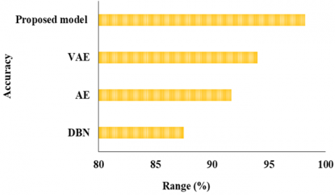
Figure 8. ACC of 70:30 ratio classification
Figure 9. Analysis of PR and RC of 70:30 ratio classification
Figure 10. Analysis of F1 and SPEC of 70:30 ratio classification
DBN: 87.5% ACC rate, 91% PR, 87% RC, 89% F1, and 88% SPEC were shown by DBN
AE: Achieved a 91.7% ACC rate, 92.5% PR, 92.5% RC, 93.4% F1, and 95% SPEC.
VAE: Displayed impressive results with a 94% ACC rate, 94.2% PR, 95% RC, 94.6% F1, and 96.3% SPEC.
Proposed model: Exceptional ACC rate of 98.2%, PR of 97%, RC of 97%, F1 of 97.8%, and SPEC of 97.5% outperformed others.
The suggested VAEGAN model has a novel mix of generative and discriminative characteristics, outperforming DBN, AE, and VAE. VAEGAN combines adversarial training, allowing it to better capture complicated data distributions and provide more realistic examples, in contrast to DBN, AE, and VAE, which only concentrate on encoding and decoding data. With the assistance of this adversarial component, VAEGAN is able to develop more substantial and accurate latent representations, improving its capacity to reconstruct data and create fresh samples with more accuracy and variety. Because VAEGAN data creation and reconstruction, it is a more effective and adaptable solution for a variety of work.
4.4 Classification validation based on LSTM
The following performance metrics for several classification models were seen in the study shown in Table 3 and Figures 11-15.
Table 3. Classification without LSTM
|
Models |
ACC (%) |
PR (%) |
RC (%) |
F1 (%) |
SPEC (%) |
|
DBN |
81.02 |
63.7 |
70.4 |
67.8 |
70.85 |
|
AE |
82.54 |
55.2 |
82.6 |
79.5 |
81.68 |
|
VAE |
85.38 |
83.2 |
87.6 |
86.2 |
87.50 |
|
Proposed model |
92.10 |
92.7 |
91.26 |
90.3 |
91.13 |
Figure 11. ACC analysis
Figure 12. PR validation
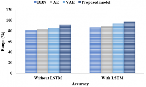
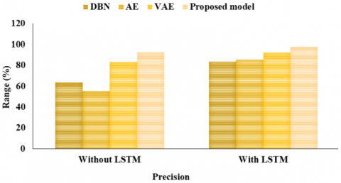
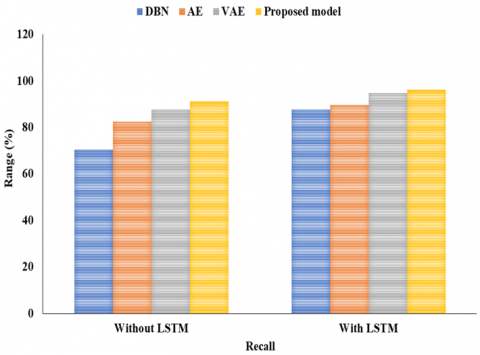
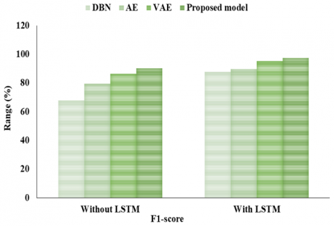
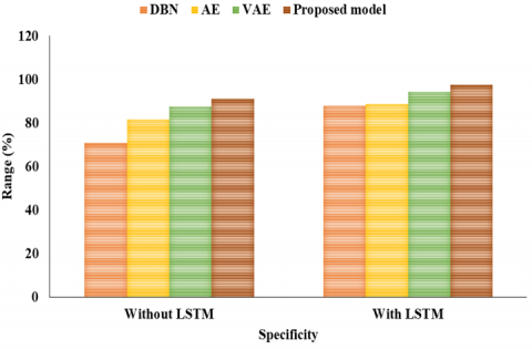
DBN earned a score of 67.8% on the F1, ACC of 81.02%, PR of 63.7%, RC of 70.4%, and Spec of 70.85%. The ACC, PR, RC, F1, and Spec of AE were 82.54%, 55.2%, 82.6%, and 79.5%, respectively. An F1 of 86.2%, an ACC of 85.38%, a PR of 83.2%, a RC of 87.6%, and a Spec of 87.50% were attained with VAE. The suggested model performed better than the others, attaining a 92.10% ACC, a 92.7% PR, a 91.26% RC, a 90.3% F1, and a 91.13% SPEC.
Figure 13. RC analysis
Figure 14. F1 validation
Figure 15. Spec analysis
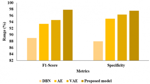
The study shown in Table 4 and Figures 11-15 compares the effectiveness of several classification algorithms using multiple metrics. With a PR of 83.7%, RC of 87.6%, F1 of 87.8%, and SPEC of 87.9%, the DBN model achieves an ACC of 86.6%. AE gets slightly better ACC, PR, RC, F1, and SPEC values of 88.6%, 85.2%, 89.5%, and 89.5%, respectively. With a high ACC of 93.9%, PR of 92.2%, RC of 94.6%, F1 of 95.2%, and SPEC of 94.4%, the VAE model, on the other hand, shows outstanding results. With an ACC of 97.8%, PR of 97.7%, RC of 96.26%, F1 of 97.3%, and Spec of 97.5%, the suggested model surpasses them all. According to these results, the suggested model performs very well in a number of areas related to forest fire detection, making it an ideal choice for this task. In LSTM feature extraction networks, weight optimisation is carried by using the MFFA. It results in improved convergence along with potentially higher ACC.
Table 4. Classification with LSTM
|
Models |
ACC (%) |
PR (%) |
RC (%) |
F1 (%) |
SPEC (%) |
|
DBN |
86.6 |
83.7 |
87.6 |
87.8 |
87.9 |
|
AE |
88.6 |
85.2 |
89.5 |
89.5 |
88.6 |
|
VAE |
93.9 |
92.2 |
94.6 |
95.2 |
94.4 |
|
Proposed model |
97.8 |
97.7 |
96.26 |
97.3 |
97.5 |
Table 5. Learning rate
|
Optimizers |
0.1 |
0.01 |
0.001 |
|
GWO |
92.13 |
95.36 |
96.22 |
|
SSA |
95.25 |
96.72 |
97.56 |
|
GSA |
97.67 |
98.69 |
98.95 |
|
Proposed model |
98 6 |
98.56 |
99.21 |
Table 5 and Figure 16 illustrates that the learning rate of our proposed model achieved ACC of 98.6% in 0.1, 98.56% in 0.01, 99.21% in 0.001. Grey wolf optimization (GWO) achieved ACC of 92.13% in 0.1, 95.36% in 0.01, 96.22% in 0.001. Sparrow search Algorithm (SSA) achieved ACC of 95.25% in 0.1, 96.72% in 0.01, 97.56% in 0.001. Grid search algorithm (GSA) achieved ACC of 97.67% in 0.1, 98.69% in 0.01, 98.95% in 0.001.
Figure 16. Learning rate graph
In conclusion, this research offerings an inclusive and cutting-edge strategy to tackle the urgent tricky of forest fires, which have become worse owing to both natural and human-caused climate changes. recognising the terrible effects that forest fires have on ecosystems, animals, and people. This study advances the accuracy and convergence of forest fire detection models by using DL approaches, such as LSTM grids for feature extraction and the use of an MFFA for weight optimisation in LSTM. Additionally, this work uses the VAEGAN model for feature classification. The WWPA, an optimisation technique inspired by nature, is used in this work to fine-tune the VAEGAN model since it is well acknowledged that hyperparameter tuning is a crucial component of model performance. The creative use of WWPA, which takes cues from plant development, makes sure that the network's parameters are efficiently optimised, eventually resulting in greater performance in detecting forest fires. The accuracy rate for the DBN model is 86.6%. With an accuracy of 88.6%, AE only slightly surpasses. The VAE model shows a high level of accuracy of 93.9%.
The recommended model, however, exceeds them all, obtaining a remarkable accuracy of 97.8%. The geographic resolution of the photos in the collection for detecting forest fires will be improved in further studies. A CNN-based image segmentation method will also be suggested in order to further alarms for the issue of forest detection. By addressing these future research directions and overcoming technical challenges, the "Detection of Forest Fire using Modified LSTM based Feature Extraction with Waterwheel Plant Optimization Algorithm based VAE-GAN model" can continue to advance and contribute to the development of more effective and reliable forest fire detection systems, ultimately aiding in the preservation of natural ecosystems and protection of public safety.
[1] Zanchi, G., Yu, L., Akselsson, C., Bishop, K., Köhler, S., Olofsson, J., Belyazid, S. (2021). Simulation of water and chemical transport of chloride from the forest ecosystem to the stream. Environmental Modelling & Software, 138: 104984. https://doi.org/10.1016/j.envsoft.2021.104984
[2] Wu, D., Zhang, C.J., Ji, L., Ran, R., Wu, H.Y., Xu, Y.M. (2021). Forest fire recognition based on feature extraction from multi-view images. Traitement du Signal, 38(3): 775-783. https://doi.org/10.18280/ts.380324
[3] Vardoulakis, S., Marks, G., Abramson, M. J. (2020). Lessons learned from the Australian bushfires: climate change, air pollution, and public health. JAMA Internal Medicine, 180(5): 635-636. https://doi.org/10.1001/jamainternmed.2020.0703
[4] Peruzzi, G., Pozzebon, A., Van Der Meer, M. (2023). Fight fire with fire: Detecting forest fires with embedded machine learning models dealing with audio and images on low power IoT Devices. Sensors, 23: 783. https://doi.org/10.3390/s23020783
[5] Srinivasan, V., Raj, V.H., Thirumalraj, A., Nagarathinam, K. (2024). Original research article detection of data imbalance in MANET network based on ADSY-AEAMBi-LSTM with DBO feature selection. Journal of Autonomous Intelligence, 7(4): 1094. https://doi.org/10.32629/jai.v7i4.1094
[6] Zheng, X., Chen, F., Lou, L., Cheng, P., Huang, Y. (2022). Real-time detection of full-scale forest fire smoke based on deep convolution neural network. Remote Sensing, 14(3): 536. https://doi.org/10.3390/rs14030536
[7] Rodrigues, M., Gelabert, P.J., Ameztegui, A., Coll, L., Vega-García, C. (2021). Has COVID-19 halted winter-spring wildfires in the Mediterranean? Insights for wildfire science under a pandemic context. Science of the Total Environment, 765: 142793. https://doi.org/10.1016/j.142793
[8] Kountouris, Y. (2020). Human activity, daylight saving time and wildfire occurrence. Science of the Total Environment, 727: 138044. https://doi.org/10.1016/j.scitotenv.2020.138044
[9] Ren, B. (2022). Neural network machine translation model based on deep learning technology. In International Conference on Multi-modal Information Analytics, Huhehaote, China, pp. 643-64. https://doi.org/10.1007/978-3-031-05237-8_79
[10] McCoy, J., Rawal, A., Rawat, D.B., Sadler, B.M. (2022). Ensemble deep learning for sustainable multimodal UAV classification. IEEE Transactions on Intelligent Transportation Systems, 24(12): 15425-15434. https://doi.org/10.1109/TITS.2022.3170643
[11] Zhang, Y., Kwong, S., Xu, L., Zhao, T. (2022). Advances in deep-learning-based sensing, imaging, and video processing. Sensors, 22(16): 6192. https://doi.org/10.3390/s22166192
[12] Hazra, A., Choudhary, P., Sheetal Singh, M. (2021). Recent advances in deep learning techniques and its applications: An overview. In Advances in Biomedical Engineering and Technology: Select Proceedings of ICBEST 2018, Raipur, India, pp. 103-122. https://doi.org/10.1007/978-981-15-6329-4_10
[13] Seo, P.H., Nagrani, A., Arnab, A., Schmid, C. (2022). End-to-end generative pretraining for multimodal video captioning. In 2022 IEEE/CVF Conference on Computer Vision and Pattern Recognition (CVPR), New Orleans, LA, USA, pp. 17938-17947. https://doi.org/10.1109/CVPR52688.2022.01743
[14] Abdusalomov, A.B., Islam, B.M.S., Nasimov, R., Mukhiddinov, M., Whangbo, T.K. (2023). An improved forest fire detection method based on the detectron2 model and a deep learning approach. Sensors, 23(3): 1512. https://doi.org/10.3390/s23031512
[15] Huang, J., He, Z., Guan, Y., Zhang, H. (2023). Real-time forest fire detection by ensemble lightweight YOLOX-L and defogging method. Sensors, 23(4): 1894. https://doi.org/10.3390/s23041894
[16] Chen, G., Zhou, H., Li, Z., Gao, Y., Bai, D., Xu, R., Lin, H. (2023). Multi-scale forest fire recognition model based on improved YOLOv5s. Forests, 14(2): 315. https://doi.org/10.3390/f14020315
[17] Zhang, L., Wang, M., Ding, Y., Bu, X. (2023). MS-FRCNN: A multi-scale faster RCNN model for small target forest fire detection. Forests, 14(3): 616. https://doi.org/10.3390/f14030616
[18] Rahman, A.K.Z.R., Sakif, S., Sikder, N., Masud, M., Aljuaid, H., Bairagi, A.K. (2023). Unmanned aerial vehicle assisted forest fire detection using deep convolutional neural network. Intelligent Automation & Soft Computing, 35(3): 3259-3277. http://dx.doi.org/10.32604/iasc.2023.030142
[19] Avazov, K., Hyun, A.E., Sami S.A.A., Khaitov, A., Abdusalomov, A.B., Cho, Y.I. (2023). Forest fire detection and notification method based on AI and IoT approaches. Future Internet, 15(2): 61. https://doi.org/10.3390/fi15020061
[20] Ye, J., Ioannou, S., Nikolaou, P., Raspopoulos, M. (2023). CNN based real-time forest fire detection system for low-power embedded devices. In 023 31st Mediterranean Conference on Control and Automation (MED), Limassol, Cyprus, pp. 137-143. https://doi.org/10.1109/MED59994.2023.10185692
[21] Al-Smadi, Y., Alauthman, M., Al-Qerem, A., Aldweesh, A., Quaddoura, R., Aburub, F., Mansour, K., Alhmiedat, T. (2023). Early wildfire smoke detection using different YOLO models. Machines, 11(2): 246. https://doi.org/10.3390/machines11020246
[22] Talaat, F.M., ZainEldin, H. (2023). An improved fire detection approach based on YOLO-v8 for smart cities. Neural Computing and Applications, 35(28): 20939-20954. https://doi.org/10.1007/s00521-023-08809-1
[23] Muhammad, K., Ahmad, J., Mehmood, I., Rho, S., Baik, S.W. (2018). Convolutional neural networks based fire detection in surveillance videos. IEEE Access, 6: 18174-18183. https://doi.org/10.1109/ACCESS.2018.2812835
[24] Khan, S., Khan, A. (2022). Ffirenet: Deep learning based forest fire classification and detection in smart cities. Symmetry, 14(10): 2155. https://doi.org/10.3390/sym14102155
[25] Adil, M., Javaid, N., Qasim, U., Ullah, I., Shafiq, M., Choi, J. G. (2020). LSTM and bat-based RUSBoost approach for electricity theft detection. Applied Sciences, 10(12): 4378. https://doi.org/10.3390/app10124378
[26] Hasan, M.N., Toma, R.N., A., Islam, M.M., Kim, J.M. (2019). Electricity theft discovery in smart grid systems: A CNN-LSTM based tactic. Energies, 12(17): 3310. https://doi.org//en12173310
[27] Aravinda, K., Santosh Kumar, Kavin, B.P., Thirumalraj, A. (2024). Traffic sign detection for practical application using hybrid deep belief network classification. In Advanced Geospatial Does in Natural Environment Resource Management, pp. 214-233. https://doi.org/10.4018/979-8-3693-1396-1.ch011
[28] Chopra, N., Ansari, M.M. (2022). Golden jackal optimization: A novel nature-inspired optimizer for engineering applications. Expert Systems with Applications, 198: 116924. https://doi.org/10.1016/j.eswa.2022.116924
[29] Dehghani, M., Montazeri, Z., Trojovská, E., Trojovský, P. (2023). Coati optimization algorithm: A new bio-inspired metaheuristic algorithm for solving optimization problems. Knowledge-Based Systems, 259: 110011. https://doi.org/10.1016/j.knosys.2022.110011
[30] Faramarzi, A., Heidarinejad, M., Mirjalili, S., Gandomi, A. H. (2020). Marine predators algorithm: A nature-inspired metaheuristic. Expert Systems with Applications, 152: 113377. https://doi.org/10.1016/j.eswa.2020.113377
[31] Abdollahzadeh, B., Gharehchopogh, F.S., Khodadadi, N., Mirjalili, S. (2022). Mountain gazelle optimizer: A new nature-inspired metaheuristic algorithm for global optimization problems. Advances in Engineering Software, 174: 103282. https://doi.org/10.1016/j.advengsoft.2022.103282
[32] Thirumalraj, A., Anandhi, R.J., Revathi, V., Stephe, S. (2024). Supply chain management using fermatean fuzzy-based decision making with ISSOA. In Convergence of Industry 4.0 and Supply Chain Sustainability, pp. 296-318. https://doi.org/10.4018/979-8-3693-1363-3.ch011
[33] Poppinga, S., Smaij, J., Westermeier, A.S., Horstmann, M., Kruppert, S., Tollrian, R., Speck, T. (2019). Prey capture analyses in the carnivorous aquatic waterwheel plant (Aldrovanda vesiculosa L., Droseraceae). Scientific Reports, 9(1): 18590. https://doi.org/10.1038/s41598-019-54857-w