Venkat Rao Kanuri*![]() | Venkata Chandra Sekhar Kasulanati
| Venkata Chandra Sekhar Kasulanati![]() | Potula Sree Brahmanandam
| Potula Sree Brahmanandam![]() | Shyam Sundar Mohan Kumar Medinty
| Shyam Sundar Mohan Kumar Medinty![]()
© 2024 The authors. This article is published by IIETA and is licensed under the CC BY 4.0 license (http://creativecommons.org/licenses/by/4.0/).
OPEN ACCESS
The study of Poiseuille flow, particularly relevant in diverse scenarios such as human blood circulation, crude oil transport, and industrial fluid dynamics, forms the crux of this research. Specifically, it delves into the analysis of fluid flow within a channel inclined at an angle relative to the horizontal axis, a scenario commonly encountered in rotating frames like bioreactors and drilling rigs, where the Coriolis force plays a crucial role. Employing the Navier-Stokes equations, this research formulates the governing equations for the flow and presents an analytical solution. It has been observed that an increase in the pressure gradient correlates with a rise in flow velocity. Furthermore, an escalation in rotational speed tends to flatten and elevate the velocity profiles. Additionally, an increase in the angle of inclination of the channel is found to boost the flow velocity. These findings have significant implications for optimizing the design and operational efficiency of systems involving inclined channels, with potential applications across various industries, including biotechnology and oil extraction.
Poiseuille flows, pressure gradient force, Coriolis force, Navier-Stokes system
Many scientific and engineering innovations, such as jet engines, drug delivery, fluidized bed reactors, aerobic granular sludge, and nuclear turbines, are premised on the understanding of fluid flow [1-3]. Flows in pipes and channels of various geometries are common in applications, and they are usually classified as Couette or Poiseuille flow. Couette flow considers flow between parallel plates that are in relative motion [4], while Poiseuille flow is flow driven by pressure difference through cylindrical channels [5]. Poiseuille flow illustrates laminar flow within constrained geometries and the conditions that the fluid is viscous, and the flow is driven by pressure variation at different points in between the parallel plates [6, 7]. In this flow regime, the force contributed by the pressure gradient and the viscous force supersedes the other inertia forces and therefore produces a uniform flow in which the fluid flow is characterized as a layer-by-layer flow. One distinguishing factor of Poiseuille flow is that its velocity profile turns out to be a symmetrical parabola whose maximum point is at the midpoint but zero on the wall [8]. The velocity gradient in this profile enhances material transport, making Poiseuille flow vital in the design and optimization of microfluidic devices. The flow of blood in the capillaries, microfluidics, and several industrial processes are some of the practical applications of the Poiseuille flow. The Poiseuile flow method makes the solution more elegant, which makes it more useful for advanced medical diagnostics, drug delivery, and chemical analysis at the microscale level. The flow of blood in the capillaries can be modeled by Poiseuille flow to explain the blood circulatory system. Fluid transport in a pipeline, heat exchanger systems, and chemical reactors are industrial processes that can be modeled by Poiseuille flow, and their applications can be found in petroleum industries and other large-scale industries [9]. Sulpizio et al. [10] studied the electron flow in channels of high-mobility graphene at high voltage. Hall field was found to be able to separate the ballistic from the hydrodynamic flow. At high temperatures, the flow presented a parabola flow velocity, thereby exhibiting the presence of Poiseuille flow. Choudhary et al. [11] studied the flow of a microswimmer under the influence of fluid inertia. The flow equations were solved using the perturbation technique. This study explores the interplay between Poiseuille flow, Coriolis force, and channel inclination. Investigating Poiseuille flow through inclined channels with Coriolis force reveals unique interactions. Three key questions are addressed in this research. The Coriolis force's impact on velocity distribution, the role of channel inclination in modifying flow, and how pressure gradients and rotational speeds affect overall behavior The findings hold significance for geophysical flows and microfluidic systems, offering insights into fluid transport systems, sediment transport predictions, and environmental phenomena.
1.1 Flows in an inclined pipe
The interaction between gravitational force and the fluid's motion in the case of an inclined channel plays a significant role in the pattern of the fluid's motion. Inclined channels are ubiquitous in both natural and engineered systems. For instance, the movement of rivers and streams through hilly terrain experiences flow variations driven by channel inclination, leading to the transport of sediment, erosion, and landscape evolution. Industrial usage for flow through an inclined channel can be found in pipelines and conduit facilities that carry fluid from a source to the destination through uneven land topographies [12-14]. Examples of such scenarios are the transport of pipe-borne water and sewage transport. The angle of inclination has been found to be very consequential in directing and redirecting the flow since the influence of gravitational force increases as the steepness increases. Masuda and Winn [15] established that increasing the angle of inclination results in higher velocities, altered pressure distributions, and complex interactions with channel boundaries.
1.2 Coriolis force
The Coriolis force is responsible for the deflection in the motion of gases or liquids due to a rotating frame. In the fundamental flow equations, the Coriolis force is just as important as the magnetohydrodynamic forces, inertial forces, and viscous forces. Physically, the forces of gravity, friction, centrifugation, and pressure gradient affect any fluid flow on the surface of the planet. In contrast, not all transport phenomena in the atmosphere and water are impacted by the Coriolis force. According to Oke et al. [16], the Coriolis force has the power to affect surface-level transport phenomena. Therefore, it is unrealistic to suppose that the Coriolis force has little impact on any non-static transport event on the surface of the globe. Three different variations in the Earth's orbit around the Sun are identified as potential mechanisms for altering the climate on a global scale. These include shifts in the equinoxes (precession), variations in the eccentricity of the Earth's orbit, and variations in the tilt of the planet's axis (obliquity) [17, 18]. Generally speaking, the rotation of the Earth has a large impact on macroscopic-scale phenomena such as air motion in the atmosphere, airplane flight, missile trajectory, and the flow of air heated by the sun. Extensive studies on the Coriolis force can be found in Oke et al. [19, 20].
1.3 Research objectives
From the ongoing study, it can be seen that Poiseuille flow has been extensively studied. To deepen the understanding of Poiseuille flow and unravel its behavior under compounded influences, the interplay between Poiseuille flow, Coriolis force, and channel inclination is studied in this paper.
In this current study, Poiseuille flow through an inclined channel in the presence of a Coriolis force is investigated. Investigation of Poiseuille flows within an inclined channel traverses new territory by investigating the interactions between two factors that counteract each other. These interactions have significant applications in geophysical flows and microfluidic systems. The unique influence of the Coriolis force includes the contortion of flow patterns, the inclination of channels affecting the balance of forces, and the interplay between pressure gradients and frame rotation. This paper provides answers to the following research questions:
In addressing these questions, we aim to establish a comprehensive understanding of fluid dynamics within rotating inclined channels. This study's implications ripple across fields, potentially shaping more effective fluid transport systems, refining predictions of sediment transport, and offering insights into environmental phenomena. As we embark on this exploration, we illuminate the intricate mechanisms governing fluid behavior, contributing to a broader understanding of the natural world and expanding the boundaries of human knowledge.
This study examines a fully developed flow involving an incompressible viscous fluid confined between two parallel plates as shown in Figure 1. The spatial arrangement is defined by the plates positioned at y=+h and y=-h creating a 2h separation between them. The restriction of flow exclusively to the x-direction and the consequential nullification of flow in the y and z directions (v=w=0) characterizes the Poiseuille flow, as visually depicted in Figure 1. The channel assumes an inclined orientation at an angle θ concerning the horizontal surface. It is essential to note that throughout this study, the channel remains non-stretching and non-shrinking. Simultaneously, it undergoes a rotational motion with an angular velocity denoted as Ω. Following the work of Jin et al. [21], the equations governing the steady flow are developed from the Navier-Stokes continuity and momentum equations given as:
$\nabla \cdot \vec{U}=0$ (1)
$(\vec{U} . \nabla) \vec{U}=-\frac{1}{\rho} \nabla p+\frac{\mu}{\rho} \nabla^2 \vec{U}+f$ (2)
Figure 1. Flow configuration
The velocity vector is $\vec{U}=(u, v, w), \rho$ and μ are the fluid density and dynamic viscosity respectively and f represents the body forces. In this case, the body forces are the Coriolis force and the gravitational force. Following the work of Koriko et al. [17], the Coriolis force is generated due to the rotation of the frame of reference and it defined as:
$F_c=-2 \vec{\Omega} \times \vec{U}$
which gives Fc=(-2Ωu,0,0). The gravitational force contribution in the flow direction is:
$F_G=(g \sin \theta, 0,0)$
where, g and θ are the gravitational acceleration and the angle of inclination respectively. Hence, the body force is:
$f_x=-2 \Omega u+g \sin \theta, f_y=f_z=0$.
The conservation law is represented in the continuity Eq. (1) and can be written in the full form as:
$\frac{\partial u}{\partial x}+\frac{\partial u}{\partial y}+\frac{\partial u}{\partial z}=0$, (3)
where, u, v and w represent the velocity components in the three dimensions. Including the body forces in the momentum Eq. (2) in the expanded form are:
$\begin{aligned} & u \frac{\partial u}{\partial x}+v \frac{\partial u}{\partial y}+w \frac{\partial u}{\partial z}=-\frac{1}{\rho} \frac{\partial p}{\partial x}+\frac{\mu}{\rho}\left(\frac{\partial^2 u}{\partial x^2}+\frac{\partial^2 u}{\partial y^2}+\frac{\partial^2 u}{\partial z^2}\right)+g \sin \theta-2 \Omega u\end{aligned}$ (4)
$u \frac{\partial v}{\partial x}+v \frac{\partial v}{\partial y}+w \frac{\partial v}{\partial z}=-\frac{1}{\rho} \frac{\partial p}{\partial y}+\frac{\mu}{\rho}\left(\frac{\partial^2 v}{\partial x^2}+\frac{\partial^2 v}{\partial y^2}+\frac{\partial^2 v}{\partial z^2}\right)$ (5)
$u \frac{\partial w}{\partial x}+v \frac{\partial w}{\partial y}+w \frac{\partial w}{\partial z}=-\frac{1}{\rho} \frac{\partial p}{\partial z}+\frac{\mu}{\rho}\left(\frac{\partial^2 w}{\partial x^2}+\frac{\partial^2 w}{\partial y^2}+\frac{\partial^2 w}{\partial z^2}\right)$ (6)
Since the channel wall is non-stretching and non-shrinking, the walls are not moving and by the no-slip condition, we have the boundary conditions at the walls as:
at $y= \pm h ; \quad u=0$.
In addition, Figure 1 shows that the maximum velocity occurs at y=0. By the condition for a stationary point, it is required that:
$\left.\frac{\partial u}{\partial y} \right\rvert\,=0$
Thus, the equations governing the flow are:
$\frac{\partial u}{\partial x}+\frac{\partial u}{\partial y}+\frac{\partial u}{\partial z}=0$ (7)
$\begin{aligned} & u \frac{\partial u}{\partial x}+v \frac{\partial u}{\partial y}+w \frac{\partial u}{\partial z}=-\frac{1}{\rho} \frac{\partial p}{\partial x}+\frac{\mu}{\rho}\left(\frac{\partial^2 u}{\partial x^2}+\frac{\partial^2 u}{\partial y^2}+\frac{\partial^2 u}{\partial z^2}\right) +g \sin \theta-2 \Omega u\end{aligned}$ (8)
$u \frac{\partial v}{\partial x}+v \frac{\partial v}{\partial y}+w \frac{\partial v}{\partial z}=-\frac{1}{\rho} \frac{\partial p}{\partial y}+\frac{\mu}{\rho}\left(\frac{\partial^2 v}{\partial x^2}+\frac{\partial^2 v}{\partial y^2}+\frac{\partial^2 v}{\partial z^2}\right)$ (9)
$u \frac{\partial w}{\partial x}+v \frac{\partial w}{\partial y}+w \frac{\partial w}{\partial z}=-\frac{1}{\rho} \frac{\partial p}{\partial z}+\frac{\mu}{\rho}\left(\frac{\partial^2 w}{\partial x^2}+\frac{\partial^2 w}{\partial y^2}+\frac{\partial^2 w}{\partial z^2}\right)$ (10)
with the boundary and initial conditions:
at $\quad y= \pm h ; \quad u=0$. (11)
at $\quad y=0 ; \quad \frac{\partial u}{\partial y}=0$. (12)
In this section, we develop the analytical solution to the Poiseuille flow through an inclined channel in a rotating frame. The flow is developed in the x-direction, so we require:
$v=w=0$. (13)
It is therefore clear that:
$\frac{\partial v}{\partial y}=\frac{\partial w}{\partial z}=0$ (14)
and substituting into the continuity equation becomes:
$\frac{\partial u}{\partial x}+\frac{\partial u}{\partial y}+\frac{\partial u}{\partial z}=0 \Rightarrow \frac{\partial u}{\partial x}=0$ (15)
Using conditions (13) and (15), we find that the momentum Eq. (8) becomes:
$\begin{gathered}u(0)+(0) \frac{\partial u}{\partial y}+(0)(0)=-\frac{1}{\rho} \frac{\partial p}{\partial x}+\frac{\mu}{\rho}\left(\frac{\partial}{\partial x}(0)+\frac{\partial^2 u}{\partial y^2}+\frac{\partial}{\partial z}(0)\right)+\rho g \sin \theta-2 \Omega u, \\ 0=-\frac{1}{\rho} \frac{\partial p}{\partial x}+\frac{\mu}{\rho} \frac{\partial^2 u}{\partial y}+\rho g \sin \theta-2 \Omega u, \frac{\mu}{\rho} \frac{\partial^2 u}{\partial y^2}-2 \Omega u=\frac{1}{\rho} \frac{\partial p}{\partial x}-\rho g \sin \theta, \frac{\partial^2 u}{\partial y^2}-\frac{2 \rho \Omega}{\mu} u=\frac{1}{\mu} \frac{\partial p}{\partial x}-\frac{g}{\mu} \sin \theta .\end{gathered}$ (16)
We turn to the remaining momentum equations and start by noting that since $v=w=0$ then:
$\frac{\partial v}{\partial x}=\frac{\partial v}{\partial y}=\frac{\partial v}{\partial z}=\frac{\partial w}{\partial x}=\frac{\partial w}{\partial y}=\frac{\partial w}{\partial z}=0$,
$\frac{\partial^2 v}{\partial x^2}=\frac{\partial^2 v}{\partial y^2}=\frac{\partial^2 v}{\partial z^2}=\frac{\partial^2 w}{\partial x^2}=\frac{\partial^2 w}{\partial y^2}=\frac{\partial^2 w}{\partial z^2}=0$
Substituting these results in the second and third momentum Eqs. (9) and (10) become:
$\begin{aligned} u(0)+(0)(0)+(0)(0) & =-\frac{1}{\rho} \frac{\partial p}{\partial y}+\frac{\mu}{\rho}((0)+(0)+(0)) \Rightarrow \frac{\partial p}{\partial y}=0\end{aligned}$ (17)
$\begin{aligned} u(0)+(0)(0)+(0)(0) & =-\frac{1}{\rho} \frac{\partial p}{\partial z}+\frac{\mu}{\rho}((0)+(0)+(0)) \Rightarrow \frac{\partial p}{\partial z}=0\end{aligned}$ (18)
Since u is invariant in the z-direction and $\frac{\partial u}{\partial x}=0$, then u=u(y). Also, Eqs. (17) and (18) show that the pressure is independent of y and z and so, p=p(x). Having established u=u(y) and p=p(x), then the partial derivatives can be dropped from Eq. (16) to become:
$\frac{d^2 u}{d y^2}-\frac{2 \rho \Omega}{\mu} u=\frac{1}{\mu} \frac{d p}{d x}-\frac{g}{\mu} \sin \theta$. (19)
The resulting Eq. (19) is a linear ordinary differential equation and the homogeneous part of the equation is:
$\frac{d^2 u}{d y^2}-\frac{2 \rho \Omega}{\mu} u=0$
whose two linearly independent solutions are:
$\frac{d^2 u}{d y^2}-\frac{2 \rho \Omega}{\mu} u=0$ (20)
where, $\alpha^2=2 \rho \Omega / \mu$. The general solution can be found by the method of undetermined coefficients. Assume the general solution is of the form
$u=A u_1+B u_2$ (21)
where, $A=A(y)$ and $B=B(y)$ and further, suppose that
$\frac{d A}{d y} u_1+\frac{d B}{d y} u_2=0$ (22)
By differentiating Eq. (21) two times we have:
$\frac{d u}{d y}=A \frac{d u_1}{d y}+B \frac{d u_2}{d y}=0$ (23)
$\frac{d^2 u}{d y^2}=A \frac{d^2 u_1}{d y^2}+B \frac{d^2 u_2}{d y^2}+\frac{d A}{d y} \frac{d u_1}{d y}+\frac{d B}{d y} \frac{d u_2}{d y}$ (24)
By substituting Eqs. (21) and (24) into Eq. (19), we have:
$\begin{gathered}A\left(\frac{d^2 u_1}{d y^2}--\frac{2 \rho \Omega}{\mu} u_1\right)+B\left(\frac{d^2 u_2}{d y^2}--\frac{2 \rho \Omega}{\mu} u_2\right)+\frac{d A}{d y} \frac{d u_1}{d y} \\ +\frac{d B}{d y} \frac{d u_2}{d y}=\frac{1}{\mu} \frac{d p}{d x}-\frac{g}{\mu} \sin \theta\end{gathered}$ (25)
Since u1 and u2 are solutions of the homogeneous equation, then
$\frac{d^2 u_1}{d y^2}--\frac{2 \rho \Omega}{\mu} u_1=0$
$\frac{d^2 u_2}{d y^2}--\frac{2 \rho \Omega}{\mu} u_2=0$
and so, Eq. (25) becomes:
$\frac{d A}{d y} \frac{d u_1}{d y}+\frac{d B}{d y} \frac{d u_2}{d y}=\frac{1}{\mu} \frac{d p}{d x}-\frac{g}{\mu} \sin \theta$
Substituting u1 and u2 as in Eq. (20), then:
$\alpha e^{\alpha y} \frac{d A}{d y}-\alpha e^{-\alpha y} \frac{d B}{d y}=\frac{1}{\mu} \frac{d p}{d x}-\frac{g}{\mu} \sin \theta$
Hence, we are required to solve the system of equations:
$e^{\alpha y} \frac{d A}{d y}+e^{-\alpha y} \frac{d B}{d y}=0$
$\alpha e^{\alpha y} \frac{d A}{d y}-\alpha e^{-\alpha y} \frac{d B}{d y}=\frac{1}{\mu} \frac{d p}{d x}-\frac{g}{\mu} \sin \theta$
Which can be written in matrix form as:
$\left(\begin{array}{cc}e^{\alpha y} & e^{-\alpha y} \\ \alpha e^{\alpha y} & -\alpha e^{-\alpha y}\end{array}\right)\left(\begin{array}{l}\frac{d A}{d y} \\ \frac{d B}{d y}\end{array}\right)=\left(\begin{array}{c}0 \\ \frac{1}{\mu} \frac{d p}{d x}-\frac{g}{\mu} \sin \theta\end{array}\right)$
$\left(\begin{array}{c}\frac{d A}{d y} \\ \frac{d B}{d y}\end{array}\right)=-\frac{1}{2 \alpha}\left(\begin{array}{cc}-\alpha e^{-\alpha y} & -e^{-\alpha y} \\ -\alpha e^{\alpha y} & e^{\alpha y}\end{array}\right)\left(\frac{1}{\mu} \frac{d p}{d x}-\frac{g}{\mu} \sin \theta\right)$
$\frac{d}{d y}\left(\begin{array}{l}A \\ B\end{array}\right)=\left(\begin{array}{l}\frac{1}{2 \mu}\left(\frac{1}{\mu} \frac{d p}{d x}-\frac{g}{\mu} \sin \theta\right) e^{-\alpha y} \\ -\frac{1}{2 \mu}\left(\frac{1}{\mu} \frac{d p}{d x}-\frac{g}{\mu} \sin \theta\right) e^{\alpha y}\end{array}\right)$
On integrating both sides,
$\int \frac{d}{d y}\left(\begin{array}{l}A \\ B\end{array}\right) d y=\left(\begin{array}{l}\frac{1}{2 \mu}\left(\frac{1}{\mu} \frac{d p}{d x}-\frac{g}{\mu} \sin \theta\right) \int e^{-\alpha y} d y \\ -\frac{1}{2 \mu}\left(\frac{1}{\mu} \frac{d p}{d x}-\frac{g}{\mu} \sin \theta\right) \int e^{\alpha y} d y\end{array}\right)$
$\left(\begin{array}{l}A \\ B\end{array}\right)=\left(\begin{array}{l}-\frac{1}{2 \alpha^2}\left(\frac{1}{\mu} \frac{d p}{d x}-\frac{g}{\mu} \sin \theta\right) e^{-\alpha y}+C_1 \\ -\frac{1}{2 \alpha^2}\left(\frac{1}{\mu} \frac{d p}{d x}-\frac{g}{\mu} \sin \theta\right) e^{\alpha y}+C_2\end{array}\right)$
Hence,
$A=-\frac{1}{2 \alpha^2}\left(\frac{1}{\mu} \frac{d p}{d x}-\frac{g}{\mu} \sin \theta\right) e^{-\alpha y}+C_1$
$B=-\frac{1}{2 \alpha^2}\left(\frac{1}{\mu} \frac{d p}{d x}-\frac{g}{\mu} \sin \theta\right) e^{\alpha y}+C_2$
Hence, the general solution for the velocity is:
$\begin{aligned} u & =\left(-\frac{1}{2 \alpha^2}\left(\frac{1}{\mu} \frac{d p}{d x}-\frac{g}{\mu} \sin \theta\right) e^{-\alpha y}+C_1\right) e^{\alpha y}+ \left(-\frac{1}{2 \alpha^2}\left(\frac{1}{\mu} \frac{d p}{d x}-\frac{g}{\mu} \sin \theta\right) e^{\alpha y}+C_2\right) e^{-\alpha y} =C_1 e^{\alpha y}+C_2 e^{-\alpha y}-\frac{1}{\alpha^2 \mu}\left(\frac{d p}{d x}-g \sin \theta\right) =C_1 e^{\alpha y}+C_2 e^{-\alpha y}-\frac{1}{2 \rho \Omega}\left(\frac{d p}{d x}-g \sin \theta\right)\end{aligned}$
Using the boundary condition u=0 when $y= \pm h$:
$\begin{aligned} & 0=C_1 e^{\alpha h}+C_2 e^{-\alpha h}-\frac{1}{2 \rho \Omega}\left(\frac{d p}{d x}-g \sin \theta\right) \Rightarrow C_1 e^{\alpha h}+C_2 e^{-\alpha h}=\frac{1}{2 \rho \Omega}\left(\frac{d p}{d x}-g \sin \theta\right)\end{aligned}$ (26)
The second condition du/dy=0 when y=0,
$\frac{d}{d y} u=\alpha C_1 e^{\alpha y}-\alpha C_2 e^{-\alpha y} \Rightarrow 0=\alpha C_1-\alpha C_2 \Rightarrow C_1=C_2$ (27)
Substituting C1=C2 into Eq. (26), we have:
$C_1\left(e^{\alpha h}+e^{-\alpha h}\right)=\frac{1}{2 \rho \Omega}\left(\frac{d p}{d x}-g \sin \theta\right)$
$C_1=\frac{1}{4 \rho \Omega \cosh (\alpha h)}\left(\frac{d p}{d x}-g \sin \theta\right)=C_2$.
Hence, we have:
$\begin{gathered}u=\frac{1}{4 \rho \Omega \cosh (\alpha h)}\left(\frac{d p}{d x}-g \sin \theta\right)\left(e^{\alpha y}+e^{-\alpha y}\right) -\frac{1}{2 \rho \Omega}\left(\frac{d p}{d x}-g \sin \theta\right) =\frac{\cosh (\alpha y)}{2 \rho \Omega \cosh (\alpha h)}\left(\frac{d p}{d x}-g \sin \theta\right)-\frac{1}{2 \rho \Omega}\left(\frac{d p}{d x}-g \sin \theta\right) =\frac{1}{2 \rho \Omega}\left(\frac{d p}{d x}-g \sin \theta\right)\left(\frac{\cosh (\alpha y)}{\cosh (\alpha h)}-1\right) .\end{gathered}$
The velocity profile generated from the analytical solution is shown in Figure 2. The graph turns out to be a parabola which is the expected shape of the velocity profile for a Poiseuille flow. The parabolic nature of the velocity indicates that the flow has the highest velocity along the line y=0 and the velocity reduces farther away from the centre.
The flow rate Q defined as:
$Q=\int_{-h}^h u d y$ (28)
is obtained as:
$\begin{gathered}Q=\frac{1}{2 \rho \Omega}\left(\frac{d p}{d x}-g \sin \theta\right) \int_{-h}^h\left(\frac{\cosh (\alpha y)}{\cosh (\alpha h)}-1\right) d y =\frac{1}{\rho \Omega}\left(\frac{d p}{d x}-g \sin \theta\right)\left(\frac{\sinh (\alpha h)}{\alpha \cosh (\alpha h)}-h\right) =\frac{1}{\rho \Omega}\left(\frac{\sinh (\alpha h)}{\alpha \cosh (\alpha h)}-h\right) \frac{d p}{d x}-\frac{1}{\rho \Omega}\left(\frac{\sinh (\alpha h)}{\alpha \cosh (\alpha h)}-h\right) g \sin \theta .\end{gathered}$
This shows a linear relationship between the flow rate and the pressure gradient with a slop of $\frac{1}{\rho \Omega}\left(\frac{\sinh (\alpha h)}{\alpha \cosh (\alpha h)}-h\right)$
Figure 2. Velocity profile
The flow of water through the inclined channel in a rotating frame is considered. The physical properties of water are given in Table 1.
Table 1. Physical properties of water
|
Property |
Symbol |
Value |
Dimension |
|
Density |
ρ |
1000 |
kg/m2 |
|
Viscosity |
μ |
0.001 |
kgm-1s-1 |
Other parameters are set to default values:
$\begin{gathered}h=0.1 \mathrm{~m}, \Omega=0.0004 \mathrm{rad} / \mathrm{s},-\frac{d p}{d x}=100 \mathrm{~Pa} / \mathrm{m} \\ g=9.81 \mathrm{~ms}^{-2}, \theta=\frac{\pi}{4}\end{gathered}$
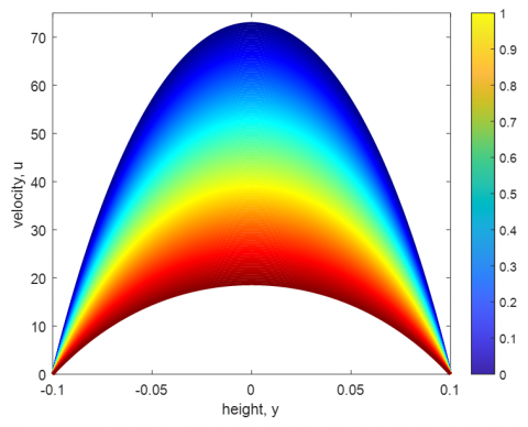
Figure 3 shows the response of velocity to decreasing pressure gradient. The pressure gradient is decreased from 100 Pa/m to 0 Pa/m and the colour map shows the gradation from blue to red; indicating that velocity is high when the pressure gradient is high but low when the pressure gradient is low. This is in agreement with Bernoulli’s principle and has been established in the literature. Fluids flow from regions of high pressure to the regions with lower pressure and hence, higher pressure gradients essentially increase the force driving the flow forward and consequently the flow velocity. Therefore, the flow velocity increases as the pressure difference increases.
Figure 4 depicts the response of flow velocity to the increasing rate of rotation. The channel under consideration is suspended over a rotating frame in such a way that the channels are irrotational. The frame rotates at an angular velocity Ω and Figure 4, shows that velocity increases with increasing rotation. The velocity profiles flatten out at the top as the rotation increases and this shows that the viscous boundary layer thickness reduces with increasing rotation. By increasing rotation from 0.0001rad/s to 0.005rad/s, the fluid gains more acceleration.
Figure 3. Velocity with pressure gradient
Figure 4. Velocity with rotation
Figure 5. Velocity with the inclination angle
The channel is set up so that it is inclined to the horizontal at an angle θ. Figure 5 shows the variation in the flow velocity as the angle of inclination increases from 0° (perfectly horizontal) to 90° (perfectly vertical). As the channel becomes more vertical, the effects of gravitational force become more significant and the force driving the flow forward increases, hence the flow velocity increases with increasing angle of inclination. The fastest flow occurs when the channel is at an angle of 90° to the horizontal.
A practical quantity of interest in the Poiseuille flow is the flow rate Q which measures the amount of fluid that passes a cross-sectional area at any time. Figure 6 shows the response of flow rate to change in pressure gradient. It can be seen that the flow rate follows a linear relationship with the pressure gradient. Considering the direction of the graph in Figure 6. it can be inferred that the slope is positive. The positive slope of the graph depicts an increasing flow rate as the pressure gradient increases. Also, the maximum flow rate is achieved when the angle of inclination is 90°. Figure 7 shows the flow rate behaviour as the radius of the channel increases. From the figure, flow rate increases as the distance separating the channel increases. Furthermore, by observing Figures 6 and 7. it can be seen that the flow rate is maximum when the channel is perfectly vertical and the flow is downward θ=90°.
Figure 6. Flow rate with pressure gradient
Figure 7. Flow rate with channel radius
In this study, the motion of the fluid through a channel inclined at an angle to the horizontal axis is investigated. The flow within the channel walls, separated by a distance of 2h is happening in a frame rotating at an angular velocity Ω. The equations governing the flow are formulated as with Navier-Stokes equations and an analytical solution is obtained for the governing equation. The results are graphed and the following outcomes are observed:
|
g |
Acceleration due to gravity |
|
p |
Pressure |
|
$\vec{U}$ |
Flow velocity vector |
|
Greek symbols |
|
|
ρ |
Density |
|
Ω |
Angular velocity |
|
θ |
Angle of inclination |
|
μ |
Dynamic viscosity, kg. m-1.s-1 |
[1] Viswanathan, H.S., Ajo‐Franklin, J., Birkholzer, J.T., Carey, J.W., Guglielmi, Y., Hyman, J.D., Karra, S., Pyrak‐Nolte, L.J., Rajaram, H., Srinivasan, G. and Tartakovsky, D.M. (2022). From fluid flow to coupled processes in fractured rock: Recent advances and new frontiers. Reviews of Geophysics, 60(1): e2021RG000744. https://doi.org/10.1029/2021RG000744
[2] Qin, L., Zhang, X., Zhai, C., Lin, H., Lin, S., Wang, P. and Li, S. (2022). Advances in liquid nitrogen fracturing for unconventional oil and gas development: A review. Energy & Fuels, 36(6): 2971-2992. https://doi.org/10.1021/acs.energyfuels.2c00084
[3] Xu, D., Li, J., Liu, J., Qu, X., Ma, H. (2022). Advances in continuous flow aerobic granular sludge: A review. Process Safety and Environmental Protection, 163: 27-35. https://doi.org/10.1016/j.psep.2022.05.018
[4] Coles, D. (1965). Transition in circular Couette flow. Journal of Fluid Mechanics, 21(3): 385-425. https://doi.org/10.1017/S0022112065000241
[5] Koplik, J., Banavar, J.R., Willemsen, J.F. (1988). Molecular dynamics of Poiseuille flow and moving contact lines. Physical Review Letters, 60(13): 1282. https://doi.org/10.1103/PhysRevLett.60.1282
[6] Gee, B., Gracie, R. (2022). Beyond Poiseuille flow: A transient energy-conserving model for flow through fractures of varying aperture. Advances in Water Resources, 164: 104192. https://doi.org/10.1016/j.advwatres.2022.104192
[7] bansali, M., Besagni, G., Bansal, P.K., Markides, C.N. (2022). Innovations in pulsating heat pipes: From origins to future perspectives. Applied Thermal Engineering, 203: 117921. https://doi.org/10.1016/j.applthermaleng.2021.117921
[8] Wu, S., Xu, Z., Jian, R., Tian, S., Zhou, L., Luo, T., Xiong, G. (2023). Molecular alignment-mediated stick–slip Poiseuille flow of oil in graphene nanochannels. The Journal of Physical Chemistry B, 127(27): 6184-6190. https://doi.org/10.1021/acs.jpcb.3c01805
[9] Sulaimon, A.A., Sannang, M.Z., Nazar, M., Shariff, A.M. (2023). Investigating the effect of okra mucilage on waxy oil flow in pipeline. Journal of Advanced Research in Fluid Mechanics and Thermal Sciences, 107(2): 41-49. https://doi.org/10.37934/arfmts.107.2.4149
[10] Sulpizio, J.A., Ella, L., Rozen, A., Birkbeck, J., Perello, D.J., Dutta, D., Ben-Shalom, M., Taniguchi, T., Watanabe, K., Holder, T., Queiroz, R. (2019). Visualizing Poiseuille flow of hydrodynamic electrons. Nature, 576(7785): 75-79. https://doi.org/10.1038/s41586-019-1788-9
[11] Choudhary, A., Paul, S., Rühle, F., Stark, H. (2022). How inertial lift affects the dynamics of a microswimmer in Poiseuille flow. Communications Physics, 5(1): 14. https://doi.org/10.1038/s42005-021-00794-y
[12] Abbas, A., Wakif, A., Shafique, M., Ahmad, H., ul ain, Q., Muhammad, T. (2023). Thermal and mass aspects of Maxwell fluid flows over a moving inclined surface via generalized Fourier’s and Fick’s laws. Waves in Random and Complex Media, 1-27. https://doi.org/10.1080/17455030.2023.2198612
[13] Jin, X., Cheng, X., Wang, Q., Wang, B. (2023). Numerical analysis of rarefied hypersonic flows over inclined cavities. International Journal of Heat and Mass Transfer, 214: 124401. https://doi.org/10.1016/j.ijheatmasstransfer.2023.124401
[14] Harish Babu, D., Naidu, K.K., Deo, S., Satya Narayana, P.V. (2023). Impacts of inclined Lorentz forces on hybrid CNTs over an exponentially stretching sheet with slip flow. International Journal of Modelling and Simulation, 43(3): 310-324. https://doi.org/10.1080/02286203.2022.2079109
[15] Masuda, K., Winn, J.N. (2020). On the inference of a star’s inclination angle from its rotation velocity and projected rotation velocity. The Astronomical Journal, 159(3): 81. https://doi.org/10.3847/1538-3881/ab65be
[16] Oke, A.S., Eyinla, T., Juma, B.A. (2023). Effect of Coriolis force on modified Eyring Powell fluid flow. Journal of Engineering Research and Reports, 24(4): 26-34. https://doi.org/10.9734/jerr/2023/v24i4811
[17] Kọríkọ, O.K., Adegbie, K.S., Oke, A.S., Animasaun, I.L. (2020). Exploration of Coriolis force on motion of air over the upper horizontal surface of a paraboloid of revolution. Physica Scripta, 95(3): 035210. https://doi.org/10.1088/1402-4896/ab4c50
[18] Oke, A.S., Mutuku, W.N., Kimathi, M., Animasaun, I.L. (2020). Insight into the dynamics of non-Newtonian Casson fluid over a rotating non-uniform surface subject to Coriolis force. Nonlinear Engineering, 9(1): 398-411. https://doi.org/10.1515/nleng-2020-0025
[19] Oke, A.S. (2021). Coriolis effects on MHD flow of MEP fluid over a non-uniform surface in the presence of thermal radiation. International Communications in Heat and Mass Transfer, 129: 105695. https://doi.org/10.1016/j.icheatmasstransfer.2021.105695
[20] Oke, A.S. (2022). Heat and mass transfer in 3D MHD flow of EG-based ternary hybrid nanofluid over a rotating surface. Arabian Journal for Science and Engineering, 47(12): 16015-16031. https://doi.org/10.1007/s13369-022-06838-x
[21] Jin, X., Cai, S., Li, H., Karniadakis, G.E. (2021). NSFnets (Navier-Stokes flow nets): Physics-informed neural networks for the incompressible Navier-Stokes equations. Journal of Computational Physics, 426: 109951. https://doi.org/10.1016/j.jcp.2020.109951