Hemangini S. Shukla* | Hema C. Surati | Munir G. Timol
© 2020 IIETA. This article is published by IIETA and is licensed under the CC BY 4.0 license (http://creativecommons.org/licenses/by/4.0/).
OPEN ACCESS
In this paper, we had investigated MHD nanofluid flow over a linearly stretching sheet in three dimensions by considering Brownian motion and thermophoresis effect for the non-Newtonian power-law model. A nonlinear system of partial differential equations with convective boundary conditions in the governing equation is converted into the system of ordinary differential equations using deductive two-parameter group-theoretic similarity technique. System of ordinary differential equation with boundary conditions are solved numerically using MATLAB BVP4C coding. The influence of different physical parameters like power-law index, magnetic parameter, Biot number, thermophoresis parameter, stretching ratio parameter, Brownian motion parameter, Lewis number, Prandtl number on concentration, temperature and velocity are investigated with graphical presentation. It is observed that as stretching parameter ratio increases, the concentration and temperature of the fluid decrease. Two different behaviours observed for velocity profiles for different power-law indexes.
Brownian motion, convective boundary conditions, deductive two parameter group-theoretic method, MHD nanofluid flow, similarity solution, thermophoresis
The nanofluid with the property of augmented heat transfer is introduced by Choi in 1995. Nanometer-sized nanoparticles like metals Cu, Ag, Au, Metallic oxides like aluminum oxide, copper oxide , Nitrides like aluminium nitride, silicon nitride, Carbides like silicon carbide, titanium carbide, semiconductors like TiO2, SiC, and different types of carbon nanotubes like SWCNT, DWCNT, MWCNT suspended in base fluid like water, ethylene glycol, oil to make nanofluid [1]. The nanofluid is useful in different areas such as in automobiles as coolants, brake fluid and as gear lubrication, also in industrial cooling, in solar devices, in medical science as a cancer drug, as coolants in electronic devices, etc. [2]. Many researchers recently worked on nanofluid because of its wide applications in the real world.
The impact of thermophoresis and Brownian motion on Powell-Eyring nanofluid model over a linearly stretching sheet is investigated by Hayat et al. using the series solution method [3]. Hayat et al. [4] analyzed second-grade nanofluid over the exponentially stretching surface using similarity method and transformed similarity equations are solved by applying the homotopy analysis technique. Nadeem et al. [5] investigated the flow of nanofluid over an exponentially stretching surface using different types of nanoparticles. Zhao et al. [6] studied the effect of nanoparticle volume fraction on various parameters for three-dimensional nanofluid flow over a stretching sheet.
Effects of Brownian motion and thermophoresis on two- dimensional non-Newtonian power-law model of MHD nanofluid flow over a non-linear stretching sheet with zero nanoparticle mass flux boundary condition are examined by Khan M. and Khan W.A. They first applied similarity transformation and then used the shooting method to solve the converted system of ordinary differential equation numerically [7]. Two-dimensional non-Newtonian Sisko fluid model is studied by Khan et al. They examined the influence of different physical parameter on nanofluid flow with convective boundary conditions using the homotopy analysis technique [8]. Shateyi [9] had analyzed three dimensional Newtonian nanofluid flow over linearly stretching sheet under the magnetic field in porous media in the presence of Brownian motion and thermophoresis with convective boundary conditions and applied spectral relaxation method to solve transformed governing equation numerically [9]. Khan et al. analyzed heterogeneous-homogeneous chemical reactions for Sisko fluid flow in three dimensions past a bidirectional stretching sheet. Heat transfer analysis is done for Cattaneo-Christov heat flux model. They presented results for the impact of different physical parameters on fluid flow for non-integer value of flow consistancy index [10]. MHD two-dimensional Sisko nanofluid flow over a nonlinearly stretching sheet under radiation effect and chemical reactions is examined by Prasannakumara et al. They observed more effectiveness of nonlinear radiation then linear thermal radiation [11].
Most of the similarity analysis is done on a nanofluid flow by assuming similarity variables. In this paper, we deduced similarity variables systematically. Two independent variables from the governing equation are reduced by using deductive two parameter group theoretical method. Moran et al. had developed deductive group formalism for similarity analysis and also included auxiliary conditions for boundary layer problems [12, 13].
Many researchers solved different types of fluid flow problem using deductive group-theoretic similarity method to reduce independent variables [14-18].
Recently, Shukla et al. [19] analysed nanofluid flow in three dimensions over linearly stretching sheet for Newtonian fluid model using two parameter deductive group-theoretic similarity technique. Hussain et al. [20] analyzed the influence of thermal radiation for three different types of nanofluid on viscous dissipative boundary layer flow over a permeable exponentially stretching sheet under the magnetic field for two-dimensional Newtonian fluid flow using similarity method.
From the literature review, we observed that most of the work done on the Newtonian fluid model is in three dimensions and little work on two-dimensional non-Newtonian nanofluid. So, here we analyzed three- dimensional non-Newtonian nanofluid flow over a linearly stretching sheet under magnetic effect for the power-law model with convective boundary conditions.
In this paper, we applied deductive two parameter group-theoretic method and derived a complete set of similarity variables and then using these similarity variables we had converted set of partial differential equations given in governing equations into ordinary differential equations. The system consists of ordinary differential equations with given boundary conditions are solved using MATLAB BVP4C coding. The influence of different physical parameters like flow consistency index, magnetic parameter, Biot number, thermophoresis parameter, stretching ratio parameter, Brownian motion parameter, Lewis number, Prandtl number on concentration, temperature and velocity are investigated with graphical presentation.
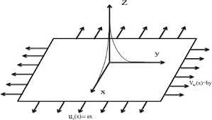
Here we had considered Non-Newtonian Power-law fluid model for steady, laminar, incompressible 3-D nanofluid flow over a linearly stretching sheet with the velocities uw=ax and vw=by, in two perpendicular directions x and y respectively (Figure 1).
$T_{\infty}$ and $C_{\infty}$ are assumed to be uniformly distributed temperature and concentration at an infinitive distance from the surface of the sheet. A hot fluid with temperature Tf is utilized to heat up or cool down the surface of the sheet by convective heat transfer mode, which provides the heat transfer coefficient hf and convective mass transfer coefficient hs. Convective concentration of fluid is Cf.
Here flow is laminar. So, uniform magnetic field B is applied to the stretched sheet in the normal direction of the surface. Here we assumed the value of Prandtl number as very small. So, the induced magnetic field can be ignored.
The equations governing by boundary layer flow are as follows [21, 22]:
$\frac{\partial u}{\partial x}+\frac{\partial v}{\partial y}+\frac{\partial w}{\partial z}=0$ (1)
$u \frac{\partial u}{\partial x}+v \frac{\partial u}{\partial y}+w \frac{\partial u}{\partial z}=-\frac{\lambda}{\rho} \frac{\partial}{\partial z}\left(-\frac{\partial u}{\partial z}\right)^{n}-\frac{\sigma B^{2}}{\rho} u$ (2)
$u \frac{\partial v}{\partial x}+v \frac{\partial v}{\partial y}+w \frac{\partial v}{\partial z}=\frac{\lambda}{\rho} \frac{\partial}{\partial z}\left[\left(-\frac{\partial u}{\partial z}\right)^{n-1} \frac{\partial v}{\partial z}\right]-\frac{\sigma B^{2}}{\rho} v$ (3)
$u \frac{\partial T}{\partial x}+v \frac{\partial T}{\partial y}+w \frac{\partial T}{\partial z}=\alpha \frac{\partial^{2} T}{\partial z^{2}}+\tau\left[D_{B}\left(\frac{\partial T}{\partial z} \frac{\partial C}{\partial z}\right)+\frac{D_{T}}{T_{\infty}}\left(\frac{\partial T}{\partial z}\right)^{2}\right]$ (4)
$u \frac{\partial C}{\partial x}+v \frac{\partial C}{\partial y}+w \frac{\partial C}{\partial z}=D_{B}\left(\frac{\partial^{2} C}{\partial z^{2}}\right)+\frac{D_{T}}{T_{\infty}} \frac{\partial^{2} T}{\partial z^{2}}$ (5)
Values at boundary are given by:
$z=0 \Rightarrow u=u_{w}=a x, v=v_{w}=b y, w=0$
$-k \frac{\partial T}{\partial z}=h_{f}\left(T_{f}-T\right),-D_{B} \frac{\partial C}{\partial z}=h_{s}\left(C_{f}-C\right)$
$z=\infty \Rightarrow u=0, v=0, w=0, T=T_{\infty}, C=C_{\infty}$ (6)
Here $u, v, w$ are velocity in the directions with respect to $x, y$ and $z .$ Symbol $T$ for the fluid temperature and $C$ for fluid concentration, $\rho$ is the fluid density, $\tau$ indicates the heat capacitance ratio, Thermophoresis diffusion coefficient is $D_{T}$ and the Brownian diffusion coefficient is $D_{B}, \lambda(>0)$ the rheological constant, flow index is $n,$ electrical conductivity of the fluid is $\sigma,$ thermal diffusivity is $\alpha .$
Figure 1. Diagram of flow system
The method used in this paper is deductive two parameter group-theoretic method. Using this method, the boundary value problem with governing Eq. (1)-(5) which has three independent variables x, y and z transformed into boundary value problem in only one independent variable, which is called similarity equation. Following is the group of transformation with two parameters (b1, b2) in the form of
$\mathrm{G}: \overline{\mathrm{s}}=r^{\mathrm{s}}\left(b_{1}, b_{2}\right) s+e^{\mathrm{s}}\left(b_{1}, b_{2}\right)$ (7)
where, s is for variable x, y, z and u, v, w, T, C.
rsand es are differentiable functions in their real arguments (b1, b2) and real-valued.
3.1 Derivation of absolute invariants
Chain rule is used to derive derivatives of the transformation defined in group G.
$\overline{\mathrm{S}}_{\bar{\imath}}=\frac{r^{\mathrm{S}}}{r^{\mathrm{i}}} s_{i}, \overline{\mathrm{S}}_{\bar{l} J}=\frac{r^{\mathrm{S}}}{r^{\mathrm{i}} r^{\mathrm{j}}} s_{i j}$ (8)
where, i and j stands for x, y, z and s stands for u, v, w, T, C .
Eq. (1) to (5) remain invariant under group of transformations defined by G in Eq. (7) and derivatives in Eq. (8).
$\frac{\partial \bar{u}}{\partial \bar{x}}+\frac{\partial \bar{v}}{\partial \bar{y}}+\frac{\partial \bar{w}}{\partial \bar{z}}=H\left(b_{1}, b_{2}\right)\left(\frac{\partial u}{\partial x}+\frac{\partial v}{\partial y}+\frac{\partial w}{\partial z}\right)$ (9)
$\bar{u} \frac{\partial \bar{u}}{\partial \bar{x}}+\bar{v} \frac{\partial \bar{u}}{\partial \bar{y}}+\bar{w} \frac{\partial \bar{u}}{\partial \bar{z}}+\frac{\lambda}{\rho} \frac{\partial}{\partial \bar{z}}\left(-\frac{\partial \bar{u}}{\partial \bar{z}}\right)^{n}+\frac{\sigma B^{2}}{\rho} \bar{u}$ $=I\left(b_{1}, b_{2}\right)\left(u \frac{\partial u}{\partial x}+v \frac{\partial u}{\partial y}+w \frac{\partial u}{\partial z}\right.$
$\left.+\frac{\lambda}{\rho} \frac{\partial}{\partial z}\left(-\frac{\partial u}{\partial z}\right)^{n}+\frac{\sigma B^{2}}{\rho} u\right)$
$+J\left(b_{1}, b_{2}\right)$ (10)
$\bar{u} \frac{\partial \bar{v}}{\partial \bar{x}}+\bar{v} \frac{\partial \bar{v}}{\partial \bar{y}}+\bar{w} \frac{\partial \bar{v}}{\partial \bar{z}}-\frac{\lambda}{\rho} \frac{\partial}{\partial \bar{z}}\left[\left(-\frac{\partial \bar{u}}{\partial \bar{z}}\right)^{n-1} \frac{\partial \bar{v}}{\partial \bar{z}}\right]+\frac{\sigma B^{2}}{\rho} \bar{v}=$
$L\left(b_{1}, b_{2}\right)\left(u \frac{\partial v}{\partial x}+v \frac{\partial v}{\partial y}+w \frac{\partial v}{\partial z}-\frac{\lambda}{\rho} \frac{\partial}{\partial z}\left[\left(-\frac{\partial u}{\partial z}\right)^{n-1} \frac{\partial v}{\partial z}\right]+\right.$
$\left.\frac{\sigma B^{2}}{\rho} v\right)+M\left(b_{1}, b_{2}\right)$ (11)
$\begin{aligned} \bar{u} \frac{\partial \bar{T}}{\partial \bar{x}}+\bar{v} \frac{\partial \bar{T}}{\partial \bar{y}}+\bar{w} & \frac{\partial \bar{T}}{\partial \bar{z}}-\alpha_{n f} \frac{\partial^{2} \bar{T}}{\partial \bar{z}^{2}}-\tau\left[D_{B}\left(\frac{\partial \bar{T}}{\partial \bar{z}} \frac{\partial \bar{C}}{\partial \bar{z}}\right)\right.\\ &\left.+\frac{D_{T}}{T_{\infty}}\left(\frac{\partial \bar{T}}{\partial \bar{z}}\right)^{2}\right] \end{aligned}$ $=N\left(b_{1}, b_{2}\right)\left(u \frac{\partial T}{\partial x}+v \frac{\partial T}{\partial y}+w \frac{\partial T}{\partial z}\right.$ $-\alpha_{n f} \frac{\partial^{2} T}{\partial z^{2}}-\tau\left[D_{B}\left(\frac{\partial T}{\partial z} \frac{\partial C}{\partial z}\right)\right.$
$\left.\left.+\frac{D_{T}}{T_{\infty}}\left(\frac{\partial T}{\partial z}\right)^{2}\right]\right)+P\left(b_{1}, b_{2}\right)$ (12)
$\begin{aligned} \bar{u} \frac{\partial \bar{C}}{\partial \bar{x}}+\bar{v} \frac{\partial \bar{C}}{\partial \bar{y}}+\bar{w} & \frac{\partial \bar{C}}{\partial \bar{z}}-D_{B}\left(\frac{\partial^{2} \bar{C}}{\partial \bar{z}^{2}}\right)-\frac{D_{T}}{T_{\infty}} \frac{\partial^{2} \bar{T}}{\partial \bar{z}^{2}} \\ &=A\left(b_{1}, b_{2}\right)\left(u \frac{\partial C}{\partial x}+v \frac{\partial C}{\partial y}+w \frac{\partial C}{\partial z}\right.\end{aligned}$ $-D_{B}\left(\frac{\partial^{2} C}{\partial z^{2}}\right)-\frac{D_{T}}{T_{\infty}} \frac{\partial^{2} T}{\partial z^{2}}$
$+E\left(b_{1}, b_{2}\right)$ (13)
The invariance of above equations implies that $J\left(b_{1}, b_{2}\right)=M\left(b_{1}, b_{2}\right)=P\left(b_{1}, b_{2}\right)=E\left(b_{1}, b_{2}\right)=0$.
This is satisfied if we take $e^{u}=e^{v}=e^{w}=0$ and
$H\left(b_{1}, b_{2}\right)=\frac{r^{u}}{r^{x}}=\frac{r^{v}}{r^{y}}=\frac{r^{w}}{r^{z}}$ (14)
$I\left(b_{1}, b_{2}\right)=\frac{\left(r^{u}\right)^{2}}{r^{x}}=\frac{r^{u} r^{v}}{r^{y}}=\frac{r^{u} r^{w}}{r^{z}}=\frac{\left(r^{u}\right)^{n}}{\left(r^{2}\right)^{n+1}}=r^{u}$ (15)
So, from Eq. (14) to (18) with boundary condition (6) we get following relations.
$\begin{aligned} L\left(b_{1}, b_{2}\right)=\frac{\left(r^{v}\right)^{2}}{r^{y}} &=\frac{r^{u} r^{v}}{r^{x}}=\frac{r^{v} r^{w}}{r^{z}}=\frac{\left(r^{u}\right)^{n-1} r^{v}}{\left(r^{2}\right)^{n+1}} \\ &=r^{v} \end{aligned}$ (16)
$\begin{aligned} N\left(b_{1}, b_{2}\right)=\frac{r^{u} r^{T}}{r^{x}} &=\frac{r^{v} r^{T}}{r^{y}}=\frac{r^{w} r^{T}}{r^{z}}=\frac{r^{T}}{\left(r^{z}\right)^{2}}=\frac{r^{T} r^{C}}{\left(r^{z}\right)^{2}} \\ &=\left(\frac{r^{T}}{r^{z}}\right)^{2} \end{aligned}$ (17)
$A\left(b_{1}, b_{2}\right)=\frac{r^{u} r^{C}}{r^{x}}=\frac{r^{v} r^{C}}{r^{y}}=\frac{r^{w} r^{C}}{r^{z}}=\frac{r^{C}}{\left(r^{z}\right)^{2}}=\left(\frac{r^{T}}{r^{z}}\right)^{2}$ (18)
So, from Eq. (14) to (18) with boundary condition (6) we get following relations.
$r^{u}=r^{x}, r^{v}=r^{y}, r^{w}=r^{z}=\left(r^{x}\right)^{\frac{n-1}{n+1}}, r^{c}=1$
$e^{u}=e^{x}=e^{v}=e^{y}=e^{w}=e^{z}=e^{T}=e^{C}=0$ (19)
Thus, we obtained a two-parameter group transformation of the form
$\mathrm{G}:\left\{\begin{array}{c}\bar{x}=r^{x} x \\ \bar{y}=r^{y} y \\ \bar{z}=\left(r^{x}\right)^{\frac{n-1}{n+1}} z \\ \bar{u}=r^{x} u \\ \bar{v}=r^{y} v \\ \bar{w}=\left(r^{x}\right)^{\frac{n-1}{n+1}} w \\ \bar{T}=T, \bar{C}=C\end{array}\right.$ (20)
3.2 The complete set of absolute invariants
Our aim is to derive proper absolute invariants such that the set of partial differential equations get transformed into a set of an ordinary differential equation. For this deduction, we applied the deductive group-theoretic method of Moran and Gaggioli. It is to be noted that the theorem due to Moran and Gaggioli states that a function gj yields the absolute invariant for two-parameter group transformations if it satisfies the following first-order linear differential equation:
$\begin{aligned}\left(\alpha_{1} x+\alpha_{2}\right) \frac{\partial g}{\partial x}+&\left(\alpha_{3} y+\alpha_{4}\right) \frac{\partial g}{\partial y}+\left(\alpha_{5} z+\alpha_{6}\right) \frac{\partial g}{\partial z} \\ &+\left(\alpha_{7} u+\alpha_{8}\right) \frac{\partial g}{\partial u} \\ &+\left(\alpha_{9} v+\alpha_{10}\right) \frac{\partial g}{\partial v} \\ &+\left(\alpha_{11} w+\alpha_{12}\right) \frac{\partial g}{\partial w} \\ &+\left(\alpha_{13} T+\alpha_{14}\right) \frac{\partial g}{\partial T} \\ &+\left(\alpha_{15} C+\alpha_{16}\right) \frac{\partial g}{\partial C}=0 \end{aligned}$ (21a)
$\begin{aligned}\left(\beta_{1} x+\beta_{2}\right) \frac{\partial g}{\partial x}+&\left(\beta_{3} y+\beta_{4}\right) \frac{\partial g}{\partial y}+\left(\beta_{5} z+\beta_{6}\right) \frac{\partial g}{\partial z} \\ &+\left(\beta_{7} u+\beta_{8}\right) \frac{\partial g}{\partial u} \\ &+\left(\beta_{9} v+\beta_{10}\right) \frac{\partial g}{\partial v} \\ &+\left(\beta_{11} w+\beta_{12}\right) \frac{\partial g}{\partial w} \\ &+\left(\beta_{13} T+\beta_{14}\right) \frac{\partial g}{\partial T} \\ &+\left(\beta_{15} C+\beta_{16}\right) \frac{\partial g}{\partial C}=0 \end{aligned}$ (21b)
where,
$\alpha_{i}=\frac{\partial r^{s_{i}}}{\partial b_{1}}\left|\left(b_{1}^{0}, b_{2}^{0}\right), \alpha_{i+1}=\frac{\partial e^{s_{i}}}{\partial b_{1}}\right|\left(b_{1}^{0}, b_{2}^{0}\right)$
$\beta_{i}=\frac{\partial r^{s_{i}}}{\partial b_{2}}\left|\left(b_{1}^{0}, b_{2}^{0}\right), \beta_{i+1}=\frac{\partial e^{s_{i}}}{\partial b_{2}}\right|\left(b_{1}^{0}, b_{2}^{0}\right)$
$(i=1,3,5,7,9,11,13,15) |$ (22)
The identity element is $\left(b_{1}^{0}, b_{2}^{0}\right)$ of the group G.
3.2.1 Independent absolute invariant
Now we obtained independent absolute invariants. From first order differential equations in (21) and (22) we get
$\left(\alpha_{1} x\right) \frac{\partial \eta}{\partial x}+\left(\alpha_{3} y\right) \frac{\partial \eta}{\partial y}+\left(\alpha_{5} z\right) \frac{\partial \eta}{\partial z}=0$
$\left(\beta_{1} x\right) \frac{\partial \eta}{\partial x}+\left(\beta_{3} y\right) \frac{\partial \eta}{\partial y}+\left(\beta_{5} z\right) \frac{\partial \eta}{\partial z}=0$ (23)
Here $\alpha_{2}=\alpha_{4}=\alpha_{6}=0$ since $e^{x}=e^{y}=e^{z}=0$
By eliminating $\frac{\partial \eta}{\partial y}, \frac{\partial \eta}{\partial x}$ from Eq. (23) we get
$\lambda_{13} x \frac{\partial \eta}{\partial x}+\lambda_{53} z \frac{\partial \eta}{\partial z}=0$
$-\lambda_{13} y \frac{\partial \eta}{\partial y}+\lambda_{51} z \frac{\partial \eta}{\partial z}=0$ (24)
where, $\lambda_{\mathrm{ij}}=\alpha_{\mathrm{i}} \beta_{\mathrm{j}}-\alpha_{\mathrm{j}} \beta_{\mathrm{i}}$.
The basic theorem of Morgan says that there exists a unique solution of the above system of equations provided the coefficient matrix is of rank two. This leads to the following cases.
Case (i): $\lambda_{53} \neq 0, \lambda_{13} \neq 0, \lambda_{51}=0$
Using the definitions of $\alpha_{i}$ 's and $\beta_{i}$ 's from (22),(23) and $\begin{array}{ll}\text { (24) } \lambda_{51}=\alpha_{5} \beta_{1}-\alpha_{1} \beta_{5}=0 & \text { (because } \alpha_{5}=\frac{n-1}{n+1} \alpha_{1}, \beta_{5}=\end{array}$ $\left.\frac{n-1}{n+1} \beta_{1}\right)$
$\frac{\partial \eta}{\partial y}=0$ (25)
$\eta$ can be expressed in variable and only.
$\eta=c_{1} z(x)^{\frac{1-n}{1+n}},$ where $c_{1}$ is an arbitrary constant.
Case (ii): $\lambda_{53}=0, \lambda_{51} \neq 0, \lambda_{13} \neq 0$
But we have $\lambda_{51}=0\left(\alpha_{5}=\frac{n-1}{n+1} \alpha_{1}, \beta_{5}=\frac{n-1}{n+1} \beta_{1}\right)$
Here the rank of the coefficient matrix is one so this case is not possible.
Case (iii): $\lambda_{53} \neq 0, \lambda_{13}=0, \lambda_{51} \neq 0$
Here also, rank is one so this case is not possible.
So, from all cases
$\eta=c_{1} z(x)^{\frac{1-n}{1+n}}$ (26)
Using same procedure we can find the absolute invariants of the dependent variables u, v, w, T and C.
3.2.2 Derivation of absolute invariants for the dependent variable u
$\left(\alpha_{1} x\right) \frac{\partial \mathrm{F}_{1}}{\partial x}+\left(\alpha_{3} y\right) \frac{\partial \mathrm{F}_{1}}{\partial y}+\left(\alpha_{7} u\right) \frac{\partial \mathrm{F}_{1}}{\partial u}=0$
$\left(\beta_{1} x\right) \frac{\partial \mathrm{F}_{1}}{\partial x}+\left(\beta_{3} y\right) \frac{\partial \mathrm{F}_{1}}{\partial y}+\left(\beta_{7} u\right) \frac{\partial \mathrm{F}_{1}}{\partial u}=0$ (27)
Eliminating $\frac{\partial \mathrm{F}_{1}}{\partial x}, \frac{\partial \mathrm{F}_{1}}{\partial y}$
$\left(\lambda_{31} y\right) \frac{\partial \mathrm{F}_{1}}{\partial y}+\left(\lambda_{71} u\right) \frac{\partial \mathrm{F}_{1}}{\partial u}=0$
$\left(-\lambda_{31} x\right) \frac{\partial \mathrm{F}_{1}}{\partial x}+\left(\lambda_{73} u\right) \frac{\partial \mathrm{F}_{1}}{\partial u}=0$ (28)
Case $(\mathrm{i}): \lambda_{31} \neq 0, \lambda_{71}=0, \lambda_{73} \neq 0$ (Because $\alpha_{1}=$ $\left.\alpha_{7}, \beta_{1}=\beta_{7}\right)$
Using the definitions of $\alpha_{i}$ 's and $\beta_{i}^{\prime}$ s from ( 22 ) we have
$\lambda_{71}=0$
$\frac{\partial \mathrm{F}_{1}}{\partial y}=0$
$\mathrm{F}_{1}(\eta)=\mathrm{F}_{1}(x, u)$ (29)
$c_{2} \mathrm{F}_{1}(\eta)=\frac{u}{x}$ (30)
$u=c_{2} x \mathrm{F}_{1}(\eta)$ (31)
Case (ii): $\lambda_{31}=0, \lambda_{71} \neq 0, \lambda_{73} \neq 0$
But we have $\lambda_{71}=0$ (Because $\alpha_{1}=\alpha_{7}, \beta_{1}=\beta_{7}$ ) Here rank of the coefficient matrix is one so this case is not possible.
Case (iii): $\lambda_{31} \neq 0, \lambda_{71} \neq 0, \lambda_{73}=0$
But we have $\lambda_{71}=0$ (Because $\alpha_{1}=\alpha_{7}, \beta_{1}=\beta_{7}$ )
Here also, rank is one so this case is not possible. Thus, we get
$u=c_{2} x \mathrm{F}_{1}(\eta)$ (32)
Similarly, we get,
$v=c_{3} y \mathrm{F}_{2}(\eta)$ (33)
$w=c_{4} F_{3}(\eta)(x)^{\frac{1-n}{1+n}}$ (34)
Similarly, we get
$\pi_{4}(\eta)=c_{5} \theta$ we choose $c_{5}=1$ and $\theta=\frac{T-T_{\infty}}{T_{f}-T_{\infty}}$ $(n)=\theta$ (35)
$\pi_{5}(\eta)=c_{6} \emptyset$ we choose $c_{6}=1$ and $\emptyset=\frac{c-c_{\infty}}{c_{f}-C_{\infty}}$ $$ \pi_{5}(\eta)=\varnothing $$ (36)
$\eta=c_{1} z(x)^{\frac{1-n}{1+n}}, \mathrm{F}_{1}(\eta)=\frac{u}{c_{2} x^{\prime}} \mathrm{F}_{2}(\eta)=\frac{v}{c_{3} y}$
$\mathrm{F}_{3}(\eta)=\frac{\mathrm{w}}{\mathrm{c}_{4}(x)^{\frac{\mathrm{n}-1}{1+1}}}, \pi_{4}(\eta)=\theta=\frac{T-T_{\infty}}{T_{f}-T_{\infty}}$
$\pi_{5}(\eta)=\emptyset=\frac{C-C_{\infty}}{C_{f}-C_{\infty}}$ (37)
Choose
$c_{1}=\left(\frac{a^{2-n}}{\frac{\lambda}{\rho}}\right)^{\frac{1}{n+1}}, c_{2}=a, c_{3}=b, c_{4}=-a\left(\frac{a^{n-2}}{\frac{\rho}{\lambda}}\right)^{\frac{1}{n+1}}$
$p r=\frac{\rho c_{p} u_{w} x}{k}(R e)^{\frac{-2}{n+1}}, R e=\frac{\left(u_{w}\right)^{2-n} x^{n} \rho}{\lambda}, \frac{\sigma B^{2}}{\rho}=M$
$B i_{1}=\frac{h_{f}}{k} x(R e)^{\frac{-1}{n+1}}, N_{b}=\tau D_{B} \frac{\left(C_{f}-C_{\infty}\right)}{\alpha}$
$N_{t}=\tau D_{T} \frac{\left(T_{f}-T_{\infty}\right)}{\alpha T_{\infty}}, L e=\frac{\alpha}{D_{B}}, B i_{2}=\frac{k}{D_{B}} x\left(R e_{b}\right)^{\frac{-1}{n+1}}$ (38)
where, $R e$ the local Reynolds number, $p r$ denotes for the generalized Prandtl number and the generalized Biot number are denoted as $B i_{1}$ and $B i_{2}, L e$ represent the Lewis number, $N_{b}$ indicates the Brownian motion parameter, $N_{t}$ represent thermophoresis parameter.
Differentiating equations in (37) with respect to $\eta$ and applying on Eq. (1) to (6), we get following
$a \mathrm{F}_{1}+b \mathrm{F}_{2}-a \mathrm{F}_{3}^{\prime}+\frac{1-n}{1+n} a \eta \mathrm{F}_{1}^{\prime}=0$ (39)
$\begin{aligned} a\left(\mathrm{F}_{1}\right)^{2}-a \mathrm{F}_{1}^{\prime} \mathrm{F}_{3}+& \frac{1-n}{1+n} a \eta \mathrm{F}_{1}^{\prime} \mathrm{F}_{1} \\ &-n a\left(-\mathrm{F}_{1}^{\prime}\right)^{n-1} \mathrm{F}_{1}^{\prime \prime}+\mathrm{MF}_{1}=0 \end{aligned}$ (40)
$\begin{aligned} b\left(\mathrm{F}_{2}\right)^{2}-a \mathrm{F}_{2}^{\prime} \mathrm{F}_{3} &+\frac{1-n}{1+n} a \mathrm{\eta} \mathrm{F}_{2}^{\prime} \mathrm{F}_{1} \\ &+a(n-1)\left(-\mathrm{F}_{1}^{\prime}\right)^{n-2} \mathrm{F}_{2}^{\prime} \mathrm{F}_{1}^{\prime \prime} \\ &-a\left(-\mathrm{F}_{1}^{\prime}\right)^{n-1} \mathrm{F}_{2}^{\prime \prime}+M \mathrm{F}_{2}=0 \end{aligned}$ (41)
$\begin{aligned} p r \pi_{4}^{\prime} \mathrm{F}_{3}-p r \frac{1-n}{1+n} \eta \mathrm{F}_{1} \pi_{4}^{\prime}+\pi_{4}^{\prime \prime}+N_{b} \pi_{4}^{\prime} \pi_{5}^{\prime} \\+& N_{t}\left(\pi_{4}^{\prime}\right)^{2}=0 \end{aligned}$ (42)
$\begin{array}{rl}\pi_{5}^{\prime \prime}+\frac{N_{t}}{N_{b}} \pi_{4}^{\prime \prime}+p r & L e \pi_{5}^{\prime} F_{3}^{\prime}-p r L e \frac{1-n}{1+n} \eta F_{1} \pi_{5}^{\prime} \\ & =0\end{array}$ (43)
with boundary conditions:
$\mathrm{F}_{1}(0)=1, \mathrm{F}_{2}(0)=1, \mathrm{F}_{3}(0)=0$
$\pi_{4}^{\prime}(0)=-B i_{1}\left(1-\pi_{4}(0)\right)$
$\pi_{5}^{\prime}(0)=-B i_{2}\left(1-\pi_{5}(0)\right)$
$\mathrm{F}_{1}(\infty)=0, \mathrm{F}_{2}(\infty)=0, \mathrm{F}_{3}(\infty)=0$
$\pi_{4}(\infty)=0, \pi_{5}(\infty)=0$ (44)
To reduce one equation choose
$\mathrm{F}_{1}=\mathrm{g}_{1}^{\prime}, \mathrm{F}_{2}=\mathrm{g}_{2}^{\prime}, \mathrm{F}_{3}=\frac{2 n}{1+n} \mathrm{g}_{1}+\frac{b}{a} \mathrm{g}_{2}+\frac{1-n}{1+n} \eta \mathrm{g}^{\prime}$ (45)
Eqns. (39)-(44) are transformed as follows.
$\begin{aligned} a\left(\mathrm{g}_{1}^{\prime}\right)^{2}-b \mathrm{g}_{1}^{\prime \prime} \mathrm{g}_{2} &-\frac{2 n}{1+n} a \mathrm{g}_{1}^{\prime \prime} \mathrm{g}_{1} \\ &-n a\left(-\mathrm{g}_{1}^{\prime \prime}\right)^{n-1} \mathrm{g}_{1}^{\prime \prime}+\mathrm{Mg}_{1}^{\prime}=0 \end{aligned}$ (46)
$\begin{aligned} b\left(\mathrm{g}_{2}^{\prime}\right)^{2}-b \mathrm{g}_{2}^{\prime \prime} \mathrm{g}_{2} &-\frac{2 n}{1+n} a \mathrm{g}_{2}^{\prime \prime} \mathrm{g}_{1} \\ &-a(n-1)\left(-\mathrm{g}_{1}^{\prime \prime}\right)^{n-2} \mathrm{g}_{2}^{\prime \prime} \mathrm{g}_{1}^{\prime \prime \prime} \\ &-a\left(-\mathrm{g}_{1}^{\prime \prime}\right)^{n-1} \mathrm{g}_{2}^{\prime \prime \prime}+M \mathrm{g}_{2}=0 \end{aligned}$ (47)
$\begin{aligned} \pi_{4}^{\prime \prime}+N_{b} \pi_{4}^{\prime} \pi_{5}^{\prime}+& N_{t}\left(\pi_{4}^{\prime}\right)^{2}+\frac{b}{a} p r \pi_{4}^{\prime} g_{2} \\ &+\frac{2 n}{1+n} p r g_{1}(\eta) \pi_{4}^{\prime}=0 \end{aligned}$ (48)
$\pi_{5}^{\prime \prime}+\frac{N_{t}}{N_{b}} \pi_{4}^{\prime \prime}+\frac{b}{a} L e p r \pi_{5}^{\prime} g_{2}+\frac{2 n}{1+n} p r L e g_{1} \pi_{5}^{\prime}$ $=0$ (49)
The bvp4c is a MATLAB solver which uses the collocation formula and a mesh of points to divide the interval of integration into subintervals. If the solution does not meet the tolerance, the solver adjusts the mesh and repeat the cycle. The BVP solver is bvp4c, which solves 2-point BVP’s using a 3-stage finite-difference Lobatto-IIIa formula which is 4th order uniformly accurate.
Kierzenka and Shampine (Kierzenka & Shampine, 2001) developed the core BVP Ordinary Differential Equation (ODE) software bvp4c to solve a large class of two-point boundary value problems of the form;
$y^{\prime}(x)=f(x, y(x), P)$ and a set of boundary conditions $g(y(a), y(b), p)=0$. Here p is a vector of unknown parameters that may, or may not, be present where f is a continuous function in y.
For Bvp4c coding we have to convert above system of equations in system of first order differential equations as follows:
Substitute $\mathrm{y}_{i},$ for $i=1,2, \ldots, 10$ for functions $\mathbf{g}_{1}, \mathbf{g}_{1}^{\prime}, \mathbf{g}_{1}^{\prime \prime}, \mathbf{g}_{2}, \mathbf{g}_{2}^{\prime}, \mathbf{g}_{2}^{\prime \prime}, \mathbf{\pi}_{4}, \mathbf{\pi}_{4}^{\prime}, \mathbf{\pi}_{5}, \mathbf{\pi}_{5}^{\prime}$ respectively
$y^{\prime}_{1}=y_{2}$ (50)
$y^{\prime}_{2}=y_{3}$ (51)
$\mathrm{y}_{3}^{\prime}=\frac{\left(a\left(\mathrm{y}_{2}\right)^{2}-b \mathrm{y}_{3} \mathrm{y}_{4}-\frac{2 n}{1+n} a \mathrm{y}_{1} \mathrm{y}_{3}+\mathrm{My}_{2}\right)}{n a\left(-\mathrm{y}_{3}\right)^{n-1}}$ (52)
$y^{\prime}_{4}=y_{5}$ (53)
$y_{5}^{\prime}=y_{6}$ (54)
$\mathrm{y}_{6}^{\prime}=\frac{b\left(\mathrm{y}_{5}\right)^{2}-b \mathrm{y}_{4} \mathrm{y}_{6}-\frac{2 n}{1+n} a \mathrm{y}_{1} \mathrm{y}_{6}-a(n-1)\left(-\mathrm{y}_{3}\right)^{n-2} \mathrm{y}_{3} \mathrm{y}_{6}+M \mathrm{y}_{5}}{a\left(-\mathrm{y}_{3}\right)^{n-1}}$ (55)
$y^{\prime}_{7}=y_{8}$ (56)
$\begin{aligned} \mathrm{y}_{8}^{\prime}=-N_{b} \mathrm{y}_{8} \mathrm{y}_{10}-& N_{t}\left(\mathrm{y}_{8}\right)^{2}-\frac{b}{a} p r \mathrm{y}_{4} \mathrm{y}_{8} \\ &-\frac{2 n}{1+n} p r \mathrm{y}_{1} \mathrm{y}_{8} \end{aligned}$ (57)
$y^{\prime}_{9}=y_{10}$ (58)
$\mathrm{y}_{10}^{\prime}=-\frac{N_{t}}{N_{b}} \mathrm{y}_{8}^{\prime}-\frac{b}{a} L e p r \mathrm{y}_{4} \mathrm{y}_{10}-\frac{2 n}{1+n} p r L e \mathrm{y}_{1} \mathrm{y}_{10}$ (59)
with boundary conditions
$\eta=0 \Rightarrow \mathrm{y}_{1}=\mathrm{y}_{4}=0, \mathrm{y}_{2}=\mathrm{y}_{5}=1$
$\mathrm{y}_{8}=-B i_{1}\left(1-\mathrm{y}_{7}(0)\right), \mathrm{y}_{10}=-B i_{2}\left(1-\mathrm{y}_{9}(0)\right)$
$\eta=\infty \Rightarrow \mathrm{y}_{1}=0, \mathrm{y}_{4}=0, \mathrm{y}_{7}=0, \mathrm{y}_{9}=0$ (60)
We obtained highly nonlinear ordinary differential equations using similarity transformations for three-dimensional non-Newtonian MHD nanofluid flow for a power-law fluid model over a linearly stretching sheet.
To solve these differential equations analytically is a very difficult task. So, here, we used bvp4c Matlab coding to get a numerical solution to the given problem. Influence on velocity, temperature, and concentration are investigated under different physical parameters.
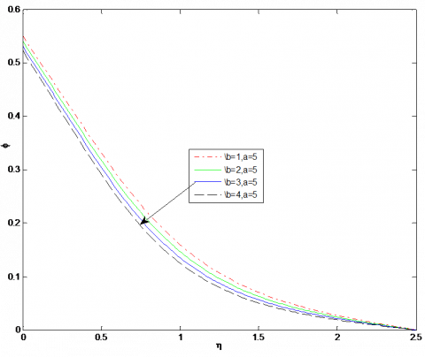
Figure 2 shows the effect of stretching parameter ratio (b/a) on concentration profile. As increasing stretching parameter ratio the concentration profile decreases.
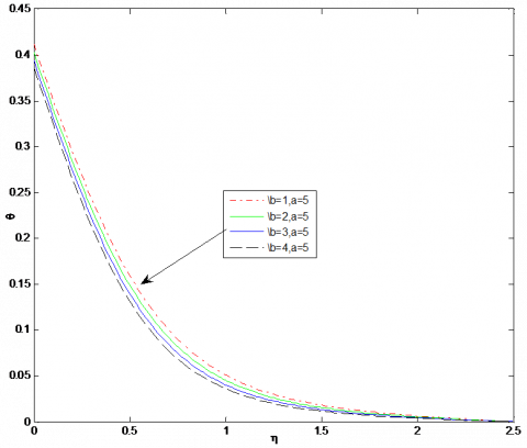
Figure 3 shows the effect of stretching parameter ratio (b/a) on temperature profile. As increasing stretching parameter ratio the temperature profile decreases.
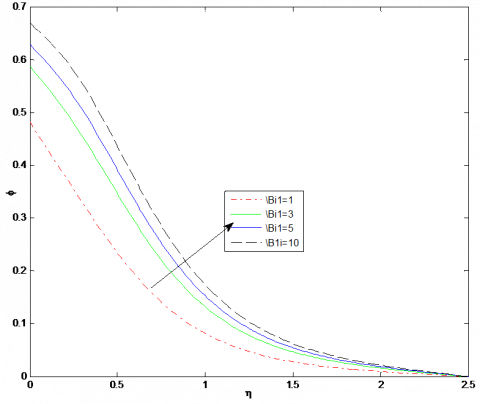
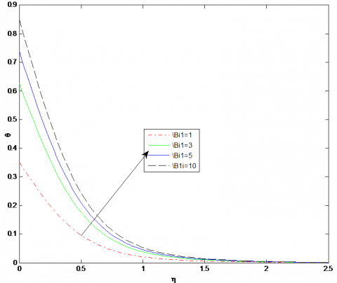
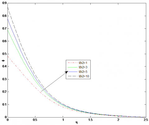
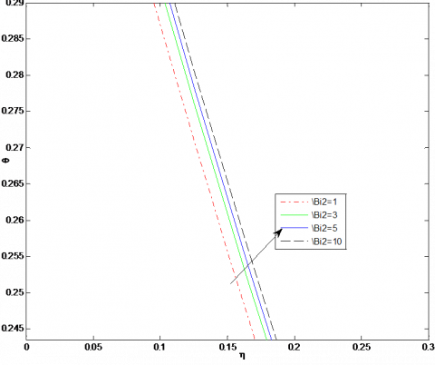
Influence of thermal Biot number and concentration Biot number on concentration and temperature profile are shown in Figure 4, 5, 6, 7. We observed an enhancement in the temperature and concentration profile for the increase in Biot numbers. Concentration Biot number is not so much affect temperature profile.
Figure 2. Effect of stretching parameter ratio (b/a) on concentration profiles for a=5, n=1, M=1, pr=2, Nb= Nt=0.2, Le=Bi1=Bi2=1
Figure 3. Effect of stretching parameter (b/a) on temperature profile for a=5, n=1, M=1, pr=2,Nb= Nt=0.2, Le=Bi1=Bi2=1
Figure 4. Effect of Biot number Bi1 on concentration profile for a=1, b=2, n=1, M=1, pr=2, Nb= Nt=0.2, Le=1, Bi2=1
Figure 5. Impact of Biot number Bi1 on temperature profile for a=1, b=2, n=1, M=1, pr=2, Nb=0.2, Nt=0.2, Le=1, Bi2=1
Figure 6. Effect of Biot number Bi2 on concentration profile for a=1, b=2, n=1, M=1, pr=2, Nb=0.2, Nt=0.2, Le=1, Bi1=1
Figure 7. Impact of Biot number Bi2 on temperature for a=1, b=2, n=1, M=1, pr=2, Nb=0.2, Nt=0.2, Le=1, Bi1=1
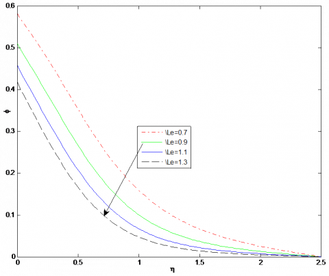
Figure 8. Influence of Lewis number Le on concentration profile for a=1, b=2, n=1, M=1, pr=2, Nb= Nt=0.2, Bi1=Bi2=1
Lewis number is inversely proportional to Brownian diffusion coefficients. So, as increasing Lewis number, Brownian diffusion decreases which decrease nanoparticle concentration. So, by increasing the value of Lewis number concentration boundary layer thickness decreases. The effect of Lewis number on concentration profile is shown in Figure 8.
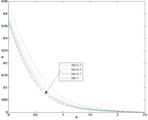
Figure 9 and 10 illustrate the behavior of concentration and temperature profile for the impact of Brownian motion parameter.
Increase in Brownian motion parameter increase temperature profile whereas decrease concentration profile. For very small nanoparticles Brownian motion is high in fluid and so the Brownian motion parameter is large. So, for large Nb nanofluid temperature enhances because of Brownian motion the kinetic energy of the particles enhances.
Figure 9. Impact of Brownian motion parameter Nb on concentration profile for a=1, b=2, n=1, M=1, pr=2, Nt=0.2, Le= Bi1=Bi2=1
Figure 10. Impact of Brownian motion parameter Nb on temperature profile for a=1, b=2, n=1, M=1, pr=2, Nt=0.2, Le=Bi1=Bi2=1
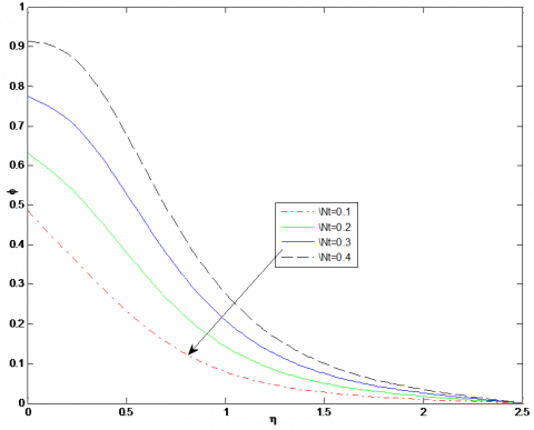
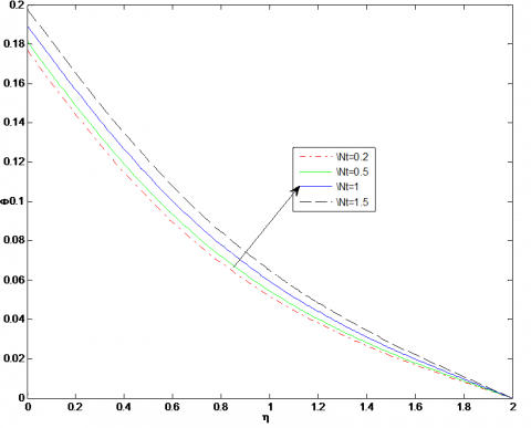
Figure 11 and 12 illustrate the behavior of concentration and temperature profile for the impact of thermophoresis parameter. Both the profile increases as increasing the thermophoresis parameter. For large values of thermophoresis parameter Nt, thermophoresis forces are produced which increase temperature and concentration.
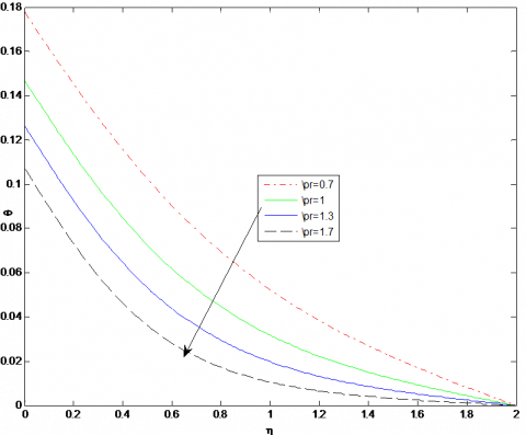
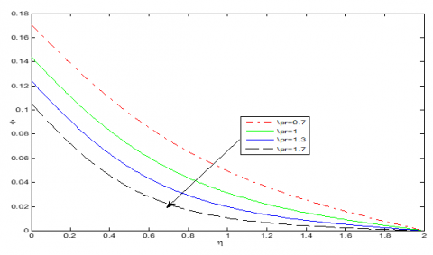
Influence of Prandtl number on temperature and concentration profile shown in Figure 13 and 14. We know that large Prandtl number has lower thermal diffusivity. So, by increasing the value of the Prandtl number, the thermal boundary layer thickness decreases. In figure temperature and concentration profile both decreases as increasing Prandtl number.
Figure 11. Influence of thermophoresis parameter Nt on concentration profile for a=1, b=2, n=1, M=1, pr=2, Nb=0.1, Le=Bi1=Bi2=1
Figure 12. Effect of thermophoresis parameter Nt on temperature profile for a=1, b=2, n=0.5, Le=2, M=1, Nb=0.1, pr=0.7, Bi1=Bi2=0.2
Figure 13. Impact of Prandtl number on temperature profile for a=1, b=2, n=0.5, Le=2, M=1, Nb=0.2, Nt=0.2, Bi1=Bi2=0.2
Figure 14. Effect of Prandtl number on concentration profile for a=1, b=2, n=0.5, M=1, Nb=0.2, Nt=0.2, Le=2, Bi1=Bi2=0.2
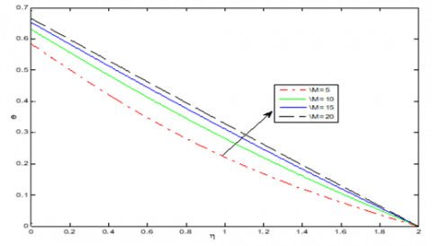
Figure 15. Influence on temperature of magnetic parameter M for a=2, b=1, n=0.5, M=5, pr=1, Nb= Nt=0.2, Le=2, Bi1=Bi2=1
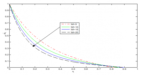
Figure 16. Influence on velocity g’1 of magnetic parameter M for a=2, b=1, n=0.5, pr=1, Nb= Nt=0.2, Le=2, Bi1=Bi2=1
Figure 17. Effect of magnetic parameter M on velocity g’2 for a=1, b=1, n=0.5, pr=1, Nb= Nt=0.2, Le=1, Bi1=Bi2=0.2
Influence on temperature and velocity profile of magnetic parameter M is shown in Figure 15, 16 and 17. By increasing value of magnetic parameter M thermal boundary layer thickness enhances and opposite behavior shown on velocity profiles. This happens because of magnetic field Lorentz force produces, which slow down the motion of fluid and increase temperature and concentration.
Figure 18. Effect of power law index on velocity g’1 for a=2, b=1, M=1, pr=1, Nb= Nt=0.2, Le=2, Bi1=1, Bi2=1
Figure 19. Effect of power law index on velocity g’1 for a=2, b=1, M=1, pr=1, Nb= Nt=0.2, Le=2, Bi1=Bi2=1
Figure 20. Influence on velocity g’2 of flow index n less than one for a=2, b=1, M=1, pr=1, Nb= Nt=0.2, Bi1=Bi2=1
Figure 21. Influence on velocity g’2 of flow index n greater than or equal to one for a=2, b=1, M=1, pr=1, Nb=0.2, Nt=0.2, Le=2, Bi1=1, Bi2=1
Impact of flow index on two velocity profile $g_{1}^{\prime}$ and $g^{\prime}_{2}$ are shown in Figure 18 to 21. For velocity $g^{\prime}_{1}$ we have two different behaviors for power law index n, near to sheet velocity profile enhances as n increases while it decreases far from the sheet and reverses the trend for velocity $g^{\prime}_{2}$.
1. Nanofluid concentration and temperature both decrease as increasing stretching ratio parameter.
2. For an increase in thermal Biot number and concentration Biot number, Nano fluid concentration and temperature both increases. Concentration Biot number has not so much influence on the temperature of nanofluid.
3. Nanofluid concentration decreases for large Lewis number.
4. Nanofluid concentration and temperature both increases as increasing thermophoresis parameter Nt.
5. Nanofluid temperature increases as the increasing value of the Brownian motion parameter whereas fluid concentration decreases as increasing value of the Brownian motion parameter.
6. A large value of Magnetic parameter enhances the fluid temperature whereas diminishing the velocity.
7. The velocity $g^{\prime}_{1}$ and the velocity $g^{\prime}_{2}$ have two different behavior for power-law index n.
|
a,b |
Positive constants |
|
B |
Applied magnetic field |
|
C |
Nanoparticle volume fraction |
|
G |
Group |
|
H, I, J, L, M, N, P, A, E |
Functions of parameters |
|
K |
Thermal conductivity |
|
Le |
Lewis number |
|
T |
Fluid temperature |
|
u, v, w |
Velocity components in directions respectvily |
|
x, y, z |
Cartesian co-ordinates |
|
pr |
Prandtl number |
|
Re |
Reynolds number |
|
Bi1, Bi2 |
The generalized Biot number |
|
DB |
Brownian diffusion coefficient |
|
DT |
Coefficient of Thermophoresis diffusion |
|
$T_{\infty}$ |
The ambient temperature far away from the surface of the sheet |
|
$C_{\infty}$ |
Concentration far away from the surface of the sheet |
|
Tf |
Convective temperature of the fluid |
|
hf |
Convective heat transfer coefficient |
|
hs |
Convective mass transfer coefficient |
|
Cf |
Convective concentration of fluid |
|
b1, b2 |
Group parameter |
|
uw, vw |
Flat surface velocity in X and Y directions |
|
$\eta$ |
Independent similarity variable |
|
$\alpha$ |
Thermal diffusivity |
|
$\lambda$ |
Positive rheological constant |
|
σ |
The electrical conductivity of the fluid |
|
$\mathcal{I}$ |
The ratio of the heat capacitance |
|
$\alpha_{i}, \beta_{i}, \lambda_{i j}$ |
constants |
[1] Choi, S.U., Eastman, J.A. (1995). Enhancing thermal conductivity of fluids with nanoparticles (No. ANL/MSD/CP-84938; CONF-951135-29). Argonne National Lab., IL (United States).
[2] Gupta, H.K., Agrawal, G.D., Mathur, J. (2012). An overview of Nanofluids: A new media towards green environment. International Journal of Environmental Sciences, 3(1): 433-440. https://doi.org/10.6088/ijes.2012030131042.
[3] Hayat, T., Ullah, I., Muhammad, T., Alsaedi, A., Shehzad, S.A. (2016). Three-dimensional flow of Powell–Eyring nanofluid with heat and mass flux boundary conditions. Chinese Physics B, 25(7): 074701. https://doi.org/10.1088/1674-1056/25/7/074701
[4] Hayat, T., Muhammad, T., Alsaedi, A., Alhuthali, M.S. (2015). Magnetohydrodynamic three-dimensional flow of viscoelastic nanofluid in the presence of nonlinear thermal radiation. Journal of Magnetism and Magnetic Materials, 385: 222-229. https://doi.org/10.1016/j.jmmm.2015.02.046
[5] Nadeem, S., Haq, R.U., Khan, Z.H. (2014). Heat transfer analysis of water-based nanofluid over an exponentially stretching sheet. Alexandria Engineering Journal, 53(1): 219-224. https://doi.org/10.1016/j.aej.2013.11.003
[6] Zhao, Q., Xu, H., Fan, T. (2015). Analysis of three-dimensional boundary-layer nanofluid flow and heat transfer over a stretching surface by means of the homotopy analysis method. Boundary Value Problems, 2015(1). https://doi.org/10.1186/s13661-015-0327-3
[7] Khan, M., Khan, W.A. (2016). MHD boundary layer flow of a power-law nanofluid with new mass flux condition. AIP Advances, 6(2): 025211. https://doi.org/10.1063/1.4942201
[8] Khan, M., Malik, R., Munir, A., Khan, W.A. (2015). Flow and heat transfer to Sisko nanofluid over a nonlinear stretching sheet. PLoS One, 10(5): e0125683. https://doi.org/10.1371/journal.pone.0125683
[9] Shateyi, S. (2017). Numerical analysis of three‐dimensional MHD nanofluid flow over a stretching sheet with convective boundary conditions through a porous medium. Nanofluid Heat and Mass Transfer in Engineering Problem. http://dx.doi.org/10.5772/65803
[10] Prasannakumara, B.C., Gireesha, B.J., Krishnamurthy, M.R., Kumar, K.G. (2017). MHD flow and nonlinear radiative heat transfer of Sisko nanofluid over a nonlinear stretching sheet. Informatics in Medicine Unlocked, 9: 123-132. http://dx.doi.org/10.1016/j.imu.2017.07.006
[11] Khan, M., Ahmad, L., Khan, W.A., Alshomrani, A.S., Alzahrani, A.K., Alghamdi, M.S. (2017). A 3D Sisko fluid flow with Cattaneo-Christov heat flux model and heterogeneous-homogeneous reactions: A numerical study. Journal of Molecular Liquids, 238: 19-26. http://dx.doi.org/10.1016/j.molliq.2017.04.059
[12] Moran, M.J., Gaggioli, R.A., Scholten, W.B. (1968). A New Systematic Formalism for Similarity Analysis, with Applications to Boundary Layer Flows. Mathematics Research Center, United States Army, University of Wisconsin.
[13] Moran, M.J., Gaggioli, R.A. (1968). Reduction of the number of variables in systems of partial differential equations, with auxiliary conditions. SIAM Journal on Applied Mathematics, 16(1): 202-215. https://doi.org/10.1137/0116018
[14] Al-Salihi, A.K., Hasmani, A.H., Timol, M.G. (2013). The new systematic procedure in group theoretic methods with applications to class of boundary layer flows. International Journal of Advances in Applied Mathematics and Mechanics, 1(1): 47-60.
[15] El-Hawary, H.M., Mahmoud, M.A., Abdel-Rahman, R.G., Elfeshawey, A.S. (2014). Group solution for an unsteady non-Newtonian Hiemenz flow with variable fluid properties and suction/injection. Chinese Physics B, 23(9): 090203. https://doi.org/10.1088/1674-1056/23/9/090203
[16] Darji, R.M., Timol, M.G. (2014). Similarity analysis for unsteady natural convective boundary layer flow of Sisko fluid. International Journal of Advances in Applied Mathematics and Mechanics, 1: 22-36.
[17] Jain, N., Timol, M.G. (2015). Similarity solutions of quasi three dimensional power law fluids using the method of satisfaction of asymptotic boundary conditions. Alexandria Engineering Journal, 54(3): 725-732. https://doi.org/10.1016/j.aej.2015.04.002
[18] Shukla, H., Patel, J., Surati, H.C., Patel, M., Timol, M.G. (2017). Similarity solution of forced convection flow of Powell-Eyring & Prandtl-Eyring fluids by group-theoretic method. Mathematical Journal of Interdisciplinary Sciences, 5(2): 151-165. https://doi.org/10.15415/mjis.2017.52012
[19] Shukla, H., Surati, H.C., Timol, M.G. (2018). Similarity analysis of three dimensional nanofluid flow by deductive group theoretic method. Applications and Applied Mathematics-An International Journal, 13(2): 1260-1272.
[20] Hussain, S.M., Sharma, R., Seth, G.S., Mishra, M.R. (2018). Thermal radiation impact on boundary layer dissipative flow of magneto-nanofluid over an exponentially stretching sheet. International Journal of Heat and Technology, 36(4): 1163-1173. https://doi.org/10.18280/ijht.360402
[21] Munir, A., Shahzad, A., Khan, M (2015). Convective flow of Sisko fluid over a bidirectional stretching surface. PloS One, 10(6): e0130342. https://doi.org/10.1371/journal.pone.0130342
[22] Nadeem, S., Haq, R.U., Akbar, N.S. (2013). MHD three-dimensional boundary layer flow of Casson nanofluid past a linearly stretching sheet with convective boundary condition. IEEE Transactions on Nanotechnology, 13(1): 109-115. https://doi.org/10.1109/TNANO.2013.2293735