Sumaryanto![]() | Sri Hery Susilowati
| Sri Hery Susilowati![]() | Ashari
| Ashari![]() | Tahlim Sudaryanto
| Tahlim Sudaryanto![]() | Mewa Ariani
| Mewa Ariani![]() | Dadan Permana*
| Dadan Permana*![]() | Agus Hadiarto
| Agus Hadiarto![]()
© 2024 The authors. This article is published by IIETA and is licensed under the CC BY 4.0 license (http://creativecommons.org/licenses/by/4.0/).
OPEN ACCESS
Considering its role on household consumption as well as production, in Indonesia chili is one of the most important vegetable commodities but also problematic in term of high risk and volatile price. Previous studies lack of detailed analyses on the factors influencing farmers' decisions to participate in chili farming and to expand their cultivation areas. Understanding farmer behavior is crucial for designing interventions that can effectively address the risks and challenges of chili farming. This study aimed to determine the behavior of farmers in chili farming. The research was conducted in one of the vegetable production centers in the Upper Citarum Watershed, West Java Province. Using the double-hurdle approach, the results show that the positive factors for the probability of participation are farmers' exposure to price volatility, the role of farming in the household economy, and positive attitudes towards vegetable farming as a way to increase income. For farmers who decided to participate, factors conducive to scaling up were self-financing, availability of family labor, and experience in vegetable farming. Results of this research imply that improvement of chili farming performance requires policy for increasing farmer access to market price, promoting contract farming, strenghtening coordination among farmers in utilising market price information for planning planting time and cropping pattern. The findings also contribute to the development of policies and practices that can improve the sustainability and profitability of chili farming.
chili farming, price volatility, risk aversion, double-hurdle
In Indonesia, Chili is one of the 12 strategic food commodities. Generally, Indonesians consume fresh chili for sauce and spices [1]. The average per capita consumption for red and cayenne chilies is 0.17 kg and 0.18 kg per annum, respectively. The participation rate and consumption of chili in 2023 have increased compared to those in 2022. Apart from direct consumption, fresh chilies are also needed by the powdered chili and dried chili industries [2].
The most popular chili cultivated in Indonesia are red chili (Capsicum annuum L) and cayenne chili (Capsicum frutescens L). The national consumption participation rate of these two types of chilies are 56.8% and 77% respectively [3].
Because chili farmers generally use conventional technology, chili production fluctuates and is sensitive to climatic conditions. As its consumption is relatively constant, the chili prices both at the retail and the farm gate are very volatile [4-7]. Red chili has the highest volatility among commodities in the volatile food group [8, 9].
Related to its contribution to inflation, the government monitors retail price movements [10]. The contribution of chili to inflation ranges between 0.01-0.07% [2]. In July 2023, red chili accounted for a monthly inflation of 0.03%. Even at the end of 2016, red chili inflation reached 138% year-on-year (yoy) [11]. Very significant fluctuations and volatility in chili prices have the potential to cause a domino effect that leads to market failure [12] that can harm farmers and consumers. High price volatility in agricultural commodities can be detrimental and become a significant problem for affected value chain actors [13].
According to the facts above, farmers face two opposing circumstances in deciding to plant chili. On the one hand, farmers are encouraged to plant chili as it has higher prices and a more significant profit than other vegetable farming [14-16]. However, farmers also run a significant risk while doing chili farming due to the high volatility of chili prices. This situation will affect farmers' decisions to choose chili cultivation or not. If the farmer decides to do chili farming, to what extent his participation in the land area will be set aside for farmers to grow chili? There are more technical considerations, in addition to economic ones, that influence farmers' decisions when it comes to planting chili.
There has been some previous research regarding farmers' decisions to plant chilies [17-19]. However, those researches were limited to determining whether farmers decide to grow chili or not and the factors that influence farmers' decisions to grow chili. Those researches did not integrate farmer participation and intensity, production, and marketing risks, in the model.
In contrast to earlier studies, with the Double Hurdle Model, our research will further explore in greater detail the farmers' participation in using land for the chili farming and the factors that influence it. Production and market risk factors that influence chili price fluctuations are analyzed in one model. The results of this analysis are crucial for the better management practices of chili farms. This paper aims to (1) analyze the determinants of farmer participation in chili farming, and (2) analyze the volatility of chili prices in the primary market.
2.1 Study site and data set
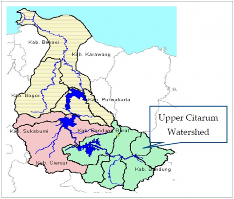
This research was conducted in the vegetable production centers of West Java Province, namely Bandung and West Bandung districts. Both districts are located in the Upper Citarum Watershed (Figure 1). In Bandung, the research locations were spread across 14 villages and 9 sub-districts, while in West Bandung, in 8 villages and 5 sub-districts.
Figure 1. Map of Citarum Watershed
The study population is comprised of farming households that cultivate vegetable commodities in at least one plot per season per year. The coverage includes farmers who work on their land or other farmers' land with the tenure status of renting, sharecropping, or mortgaging.
The data analyzed are the results of the 2019 survey in the "INDOGREEN" project, which is a research collaboration between ACIAR and The Indonesian Center for Agriculture Socio-Economic and Policy Studies (ICASEPS) under the Indonesian Ministry of Agriculture, where most of the authors are implementing the project. Using a simple random sampling method, the number of samples in the research project was 499 farming households. In this study, out of that number, 238 vegetable farming households were drawn as sub-sample.
In May 2023, Focus Group Discussions (FGDs) were conducted in several villages in the two research districts. FGDs focused on the cultivation and marketing aspects of chili peppers. FGD participants included vegetable farmers, vegetable traders, village community leaders, and field extension officers.
There is not enough farmgate price data series available for price volatility analysis. Based on the assumption of farmgate - grocer price transmission, considering its limitations, the data used in the volatility analysis is the weekly average grocer price data, which is the primary marketing destination of chili farmers in the research location, namely the provincial capital wholesale market. The data was collected from the Ministry of Trade, covering the series from the first week of January 2018 to the second week of May 2023.
2.2 Analytical methods
The farmer's decision to cultivate chili includes two stages. The first stage is the choice to cultivate or not cultivate. For those who decide to cultivate, the second stage is deciding the holding size of the cultivation. The model commonly used to analyze such conditions is double-hurdle regression because of its flexibility and appropriateness in managing overdispersion and zero-inflated data. The model allows the errors of the participation decision and the number of decisions to be correlated [20-22].
If yi represents the observed chili cultivation amount of the farmer, we can model it as:
$y_i= \begin{cases}x_i \beta+\varepsilon_i & \text { if } \min \left(x_i+\varepsilon_i, \mathbf{z}_{\mathbf{i}} \gamma+u_i\right)>0 \\ 0 & \text { otherwise }\end{cases}$
$\left(\begin{array}{c}\varepsilon_i \\ u_i\end{array}\right) \sim N(0, \Sigma), \Sigma=\left(\begin{array}{cc}1 & \sigma_{12} \\ \sigma_{12} & \sigma\end{array}\right)$
With correlation r, the log-likelihood function for the double-hurdle model is:
$\begin{aligned} & \log (L)=\sum_{y_i=0}\left[\log \left\{1-\Phi\left(z_i \gamma, \frac{x_i \beta}{\sigma}, \rho\right)\right\}\right] \\ & \quad+\sum_{y_i>0}\left(\log \left[\Phi\left\{\frac{z_i \gamma+\frac{\rho}{\sigma}\left(y_i-x_i \beta\right.}{\sqrt{1-\rho^2}}\right\}\right]\right) \\ & \quad-\sum_{y_i>0}\left(\log [\sigma]+\log \left\{\phi\left(\frac{y_i-x_i \beta}{\sigma}\right)\right\}\right)\end{aligned}$
Among various farming businesses, price fluctuations are the most economically sensitive risk [23]. The farmer often faces significant price variations when selling agricultural products, resulting in income uncertainty [24]. This issue influences farmers’ decision, taking into consideration volatility of products’ price.
Price volatility conceptually describes how often the price of a product (agriculture) changes over time. It leads to high market risks due to farmers' inability to estimate prices and potentially harms the welfare of market participants [25]. Volatility reflects overall price variability in both high and low fluctuations [26-29].
One indicator to determine price volatility is the Bollinger Band. When the width of the Bollinger Bands increases, it indicates that chili price volatility is increasing, whereas when the upper and lower bands narrow, it means low volatility. Price volatility can be faster and sharper, increasing profit opportunities and the risk of profit loss. The higher the volatility, the higher the future price uncertainty, and the higher the risk of farming, as well as the more difficult and expensive risk management by producers [30-33].
2.3 Empirical model
From a series of preliminary tests, the most suitable double-hurdle model applied in this study is as follows:
(a) Participation equation:
$\begin{aligned} & d_i^*=\alpha_0+\alpha_1 {age}_i+\alpha_2 { exper }_i+\alpha_3 { educ }_i+\alpha_4 { fmlabor }_i \\ & +\alpha_5 { attveg }_i+\alpha_6 { deccrop }_i+\alpha_7 { dcmarket }_i+\alpha_8 { pvolatil }_i \\ & +\alpha_9 { share _ ann }+\delta_1 { main_inc }+\delta_2 { District }_i+u_i \\ & \end{aligned}$
where $d_i^*=\left\{\begin{array}{l}1 . \text { if participate in chili farming } \\ 0, \text { if not participate in chili farming }\end{array}\right.$
(b) Intensity equation (land holding for chili cultivation):
$\begin{aligned} & y_i^*=\beta_0+\beta_1 { age }_i+\beta_2 { exper }_i+\beta_3 { educ }_i+\beta_4 { fmlabor }_i \\ & +\beta_5 { deccrop }_i+\beta_6 { dcmarket }_i+\beta_7 { pvolatil }_i+\beta_8 { rsavr }_i \\ & +\beta_9 { selfinv }+\beta_{10} { share _ann }+\delta_3 { cpattern }_i+v_i \\ & \end{aligned}$
where,
$y_i= \begin{cases}y_i^* & \text { if } y_i>0 \text { and } d_i^*>0 \\ 0 & \text { otherwise }\end{cases}$
and
$\left(\begin{array}{l}u_i \\ v_i\end{array}\right) \sim N(0, \Sigma), \Sigma=\left(\begin{array}{cc}1 & \sigma_{12} \\ \sigma_{12} & \sigma\end{array}\right)$
$y_i^*=$ chili farming area of farmer $-i$
where,
age = Age of household's head (HH) (years).
exper = Experience in farming, all include non- vegetable farming (years: 1= if less than 15, 2= if 16-30, 3= if > 30).
educ = Education of HH (years of schooling).
fmlabor = Number of household's member age 15 - 64 (persons).
attveg = Attitude to the role of vegetable crops farming as a whole (score):
1 = disagree or not sure that vegetable farming will significantly improve household income;
2 = agree that vegetable farming will significantly improve household income;
3 = strongly agree that vegetable farming will significantly improve household income.
deccrop = Level of concern on how to decide crops should be chosen (regrouping of score 0 - 10):
0 = never;
1 = if the score is 1 - 3;
2 = if the score is 4 - 6;
3 = if the score is 7 - 9;
4 = if the score is 10.
dcmarket = Level of concern on how to sell production (regrouping of score 0 - 10): 0 = never; 1 = if score is 1 - 3; 2 = if the score is 4 - 6; 3 = if the score is 7 - 9; 4 = if the score is 10.
pvolatil = Proxy variable deal with accessing information of vegetable's price volatility (score):
1 = low (main job is farming, second job is non-agricultural business trading); or main job is non-agricultural business and second job is farming;
2 = moderate (main job is farming, second job is agricultural trading business;
3 = high (main job is agricultural trading business, second job is farming).
Main_inc = Dummy variable (biner; 1 if contribution of income from annual crop farming include vegetable > 0.5.
riskaver = Level of risk aversion (score: 1 - 5, based on the farmer reaction to the question deal with offering to try out new tools, inputs, or farming methods in farm management):
1 = will be the first to try;
2 = was/will be one of the first groups to try;
3 = before trying, I usually wait for results from other people;
4 = usually the last person in the group to try;
5 = never tried.
selfing = Owned capital availability for farming (potential, million IDR)
cpattern = Cropping pattern of each plot per season (0=monoculture, 1=polyculture)
District = District (0=Bandung, 1=West Bandung)
The selected estimation method is maximum likelihood with clustered-robust standard errors because it is one of the most efficient, and the parameter estimation results are consistent [34-36]. The cluster used is district. The software used in parameter estimation was Stata 15.1, created by StataCorp. company, Texas, USA, whose syntax imitates [21].
The price volatility analysis applied in this study is the Bollinger Bands method. Adjusting to the empirical conditions in the field, the moving average period applied is 15 weeks, while the distance used to determine the lower and upper bands is two standard deviations.
3.1 A brief of vegetable farming in the study site
Vegetable crops are part of the total agricultural commodities grown by farmers. About 71% of the farmers also grow other annual crops, mainly rice, maize, and sweet potatoes, and about 15% of them also grow perennial crops, mainly coffee.
Most farmers cultivate more than one plot, but the plots are small. The percentages of farmers with one, two, and three or more plots are 25%, 38%, and 37%, respectively. The average cropping intensity of annual crops on the cultivated plots was 1.53 per year, ranging from 1 - 4. With such cropping intensity, including perennial crop plots, the average cultivated area of arable land per year is around 0.68 hectares (sd=0.79, min=0.06, max=4.69).
Although farming experience is positively correlated with age, it is not directly proportional. Some of them became farmers after inheriting farmland from their parents. Meanwhile, some were originally farmers and then changed their occupations to non-agricultural sectors. The distribution of farmers according to their farming experience under 15 years, between 15 and 30 years, and over 30 years is 35, 37, and 18 percent, respectively (Table 1).
Table 1. Summary statistics of variables included in the parameter estimation
|
Variables |
Mean |
Std. Dev. |
|
age (years) |
48.68 |
12.35 |
|
education (years of schooling) |
6.269 |
2.553 |
|
experience in farming (score:1 - 3) |
1.727 |
0.744 |
|
number of HH members aged 15 - 64 (persons) |
2.622 |
1.129 |
|
attitude to the role of vegetable farming (score: 1 - 3) |
2.092 |
0.595 |
|
decision making of choosing crop (score: 0 - 4) |
2.924 |
0.969 |
|
decision of choosing market channel (score: 0 - 4) |
2.710 |
1.146 |
|
level of accessing price volatility (score: 1 - 3) |
1.118 |
0.394 |
|
level of risk aversion (score: 1 - 5) |
2.235 |
1.004 |
|
owned capital availability for farming (million IDR) |
9.356 |
7.142 |
|
Share of income from annual crop farming |
0.530 |
0.308 |
|
Cropping pattern dominant: (0=monoculture, 1=polyculture) |
0.634 |
0.483 |
|
The primary source of income (0=non agriculture, 1=agriculture) |
0.748 |
0.435 |
|
District (0=Bandung, 1=West Bandung) |
0.303 |
0.460 |
|
area of chili farming (hectare) |
0.066 |
0.197 |
Regarding formal education, the number of farmers who did not complete primary school, completed primary school and junior high school are 21%, 56%, and 15%, respectively, while those who completed high school are 8%.
Due to their small cultivated area, farmers cannot rely entirely on their income from agriculture. Meanwhile, there is a positive correlation between land area and household per capita income [37]. The number of farmers whose entire household income is solely from agriculture is around 81%. However, farmers who are "sure" and "very sure" that vegetable farming can increase their income are 81% and 23%, respectively.
Per capita income per year in Bandung district is around IDR 16.7 million, while in West Bandung, it is around IDR 11.6 million. The share of income from annual crop farming, including vegetables, in Bandung district is 59%, while in West Bandung, it is 42%.
Although it is common in rural areas for people as young as 15 years old to be involved in agricultural work, there is a tendency for younger people to be more interested in working and or assisting in the off-farm work. Young farmers' perceptions of the accessibility of agricultural facilities and infrastructure significantly affect the decision and intensity of whether to engage in farm or off-farm work [38]. Under such conditions, especially for farmers whose cultivated land is above 0.3 hectares (61%), they rely on farm laborers to meet their labor needs for land cultivation, planting, and harvesting activities.
In vegetable farming, the choice of which commodities to grow and how to market them is a routine agenda to be decided in the planting season. In the rural Upper Citarum Watershed, there are 18 popular vegetable commodities. Based on the cumulative area cultivated in one year, the top five are potato (21%), cabbage (17%), tomato (15%), green onions (9%) and chili (8%). The most popular marketing channel is farmer - village/sub-district intermediary - wholesaler - primary vegetable market in the provincial capital.
In the FGDs, almost all participants concluded that in rural Upper Citarum Watershed, chili farming is the highest risk. This conclusion is confirmed by the results of data analysis from all samples in this study, which show that the coefficient of variation of profit per hectare of chili farming is around 72%. In comparison, the average for all commodities other than chili is 63%. The research by Susilowati et al. [39] and Mailena et al. [40] are consistent with the information above.
In addition to the high risk, in this region, the capital cost of chili farming is relatively the highest. Hence, the number of farmers who cultivate chili is only 24%, with an average cultivated area of 0.28 hectares. Only 17% participated in Bandung, with an average cultivated area of 0.37 hectares, while West Bandung had 39%, with an average cultivated area of 0.19 hectares.
The average income of vegetable farmers in Bandung is approximately 22.1 million IDR/hectare (sd= 13.0, min=-5.8, max=71.4 million IDR), while in West Bandung, it is about 24.3 million IDR/hectare (sd=16.9, min=-8.7, max=74.0 million IDR).
3.2 Probability and participation intensity of farmers in chili farming
Despite the higher average profit per hectare in chili farming compared to other vegetable commodities, the level of farmer participation in chili cultivation remains low at 24%. The participation rate is lower in Bandung district (19%) compared to West Bandung (39%), even though the profits per hectare in Bandung are relatively higher than in West Bandung.
In Bandung district, the average profit per hectare is approximately 29.3 million IDR sd=18.7, min= -31.83, max=71.4 million ID. Meanwhile, in West Bandung, the average profit is lower at 27.7 million IDR but with a higher dispersion (sd= 21.4, min= -8.7, max=75.0). Calculating the coefficient of variation reveals that the risk of chili farming in Bandung is relatively lower than in West Bandung (0.637 vs 0.772). However, it is important to note that farming risk is just one factor influencing the opportunity and intensity of participation, as further demonstrated by the following parameter estimation results (Table 2).
The increased participation of farmers in West Bandung can be attributed primarily to the prevailing land conditions and the implications of land and water conservation policies in the Upper Citarum Watershed. In this region, chili farming is more prevalent in paddy fields, particularly during the second planting season following rice cultivation. Additionally, West Bandung exhibits higher averages in terms of both the number of plots and the overall area of rice fields. These factors contribute to the heightened engagement of farmers in chili cultivation in West Bandung.
Farming on dry land presents notable vulnerabilities, including susceptibility to damage, sensitivity to water stress, and the potential emergence of pests and diseases. Additionally, extreme climate events such as El Nino or La Nina can lead to crop failures. Adopting adaptive technologies could be chosen to enhance the resilience of dry lands in coping with climate change [41]. Regarding land topography, most land plots (83.3%) fall within the flat to moderately steep category, with only 16.7% classified as steep, exceeding a 30% slope.
Chili can be grown in highlands or lowlands and does not require complex treatments [42-44]. In contrast to vegetable crops, which can only be harvested once during a planting cycle, chili can be harvested every two to three weeks until the harvest period of two and a half months. Cayenne chili can keep producing as long as the plant is still alive. As a result, farmers can profit continuously from growing chili. The demand for chili and the relatively high average selling price motivate farmers to plant chili [45, 46].
The conversion of farmland from vegetable farming to agroforestry in West Bandung District is slower. The conversion is prioritized on farm plots with steep slopes (slope>30%) and is a pro-conservation agricultural development strategy. Since the Upper Citarum Watershed is located in the upstream of most rural areas in Bandung Regency and the critical area is much larger, the priority scale is higher.
Engaging in intensive vegetable farming on steep slopes poses significant risks to environmental sustainability and human safety. Planting vegetables on such terrain increases the likelihood of landslides, elevating the risk of land erosion and topsoil loss. According to several studies, land erosion poses a serious concern to farmers in highlands with steep slopes [47-49]. Given these challenges, highland agricultural endeavors demand specific and careful treatment due to inherent biophysical limitations [50].
Considering its financial prospects and contribution to conservation, the most popular perennial commodity is coffee. A number of research results showed that coffee-based agroforestry systems are also popular in some African countries such as Ethiopia [51], Kenya [52], and Uganda [53] and in several countries in Latin America [54, 55].
In line with farmers' opinions during FGDs, parameter estimation results also show that farmers who rely on their household income from agriculture have a higher probability of participating in chili farming. It is also evident in this study that the higher the ability of farmers to access information on vegetable price volatility, the higher the probability of participation. For those who participate, increased access to information on price volatility encourages farmers to increase their chili cultivation area.
The limited number of samples (238) implies that the parameter estimation results with the double-hurdle model applied in this study are "plausible" if the risk aversion and self-financing ability variables are only included in the intensity equation. It appears that for participating farmers, the lower their risk aversion, the more they will expand their chili farms. Meanwhile, since the cost of chili farming per unit of the cultivated area is relatively higher than the average of other agricultural commodities (except broccoli), farmers will plant more chili if their self-financing ability is higher.
Farming is increasingly unpopular among older farmers. It is evident that age has a negative and substantial impact on the involvement and intensity equations. Whether this is due to the conservative attitude that generally prevails among older farmers or other factors cannot be concluded from this study. However, the FGDs revealed that the attitude of older farmers tends to prioritize "safety" over the expectation of high but uncertain returns.
The level of formal education has a negative effect on participation, but for farmers who decide to engage in chili farming, it does not affect the intensity. Empirically, the lower participation applies not only to chili farming but also to other annual crops. The reason is that farmers with a higher level of education tend to prioritize perennial crop farming, which is generally not labor intensive so that more time can be devoted to non-agricultural work; some even have non-agricultural as their primary occupation. It is confirmed by the effect of the labor force variable on participation. However, for farmers who decide to participate, higher family labor availability encourages them to cultivate more chili farms.
About 75% of the farmers cultivate more than one plot, and the number of farmers with more than two plots is about 34%. Cropping patterns applied to each plot vary. Cumulatively, the dominant cropping area is polyculture. For farmers participating in chili farming, the intensity of cultivation is more significant if the cumulative farming area is dominantly polyculture. It is related to the risk mitigation motive of the entire vegetable farm.
Table 2. Parameter estimate of the double hurdle participation of farmers in chili farming
|
Variables |
Participation eq. |
Intensity eq. |
||
|
Coef. |
Std. Err. |
Coef. |
Std. Err. |
|
|
Age of household's head |
-0.003*** |
0.001 |
-0.015*** |
0.005 |
|
Education of household's head |
-0.271*** |
0.084 |
0.043 |
0.040 |
|
Experience in farming (technical and management) |
-0.142 |
0.125 |
0.309*** |
0.015 |
|
Number of household members ages 15 - 64 years |
-0.196*** |
0.050 |
0.084*** |
0.018 |
|
Attitude: vegetable farming as income improvement |
0.170*** |
0.007 |
|
|
|
Understanding that crop choice is essential |
-0.382 |
0.626 |
0.070 |
0.154 |
|
Cropping pattern (0=monoculture, 1=polyculture) |
|
|
0.135** |
0.065 |
|
Level of concern about the marketing channel |
0.438 |
0.525 |
-0.087 |
0.070 |
|
Level of accessibility to vegetable price volatility |
0.339** |
0.167 |
0.018** |
0.009 |
|
Level of risk aversion |
|
|
-0.088*** |
0.007 |
|
Owned capital availability for farming |
|
|
0.022** |
0.009 |
|
Share of income from farming annual crops |
-1.345 |
0.750 |
0.020 |
0.090 |
|
The primary source of income (0=non agric,1=agric) |
0.892** |
0.430 |
|
|
|
District (0=Bandung, 1=West Bandung) |
3.423*** |
0.850 |
|
|
|
_cons |
1.645 |
2.166 |
-0.559 |
0.986 |
|
/Sigma |
0.404 |
0.136 |
|
|
|
/Covariance |
0.165** |
0.069 |
|
|
The number of obs. = 238; log likelihood = -99.2271; AIC = 200.4541; BIC = 203.9264
***: $\alpha$ = 0.01, **: $\alpha$ = 0.05
3.3 Chili price volatility and farmers' planting schedule
In the FGD in May 2023, most farmers expressed their complaints that chili prices are very volatile. Therefore, the volatility analysis focused on the following two issues: (i) the extent of the dynamics of the weekly average price in relation to the lower band - upper band range and (ii) the extent of the planting schedule applied by farmers in relation to these price dynamics.
Shocks in production and consumption can cause fluctuations in chili prices. The production shock is generally due to seasonal weather or chili production patterns (off-season and on-season). Red chili is one crop type that is highly dependent on the seasons. A shock in consumption can also cause price fluctuations from changes in people's consumption patterns on religious holidays [5]. Government policy on chili imports also influences price fluctuations [46, 56]. However, price movements due to consumption factors are closely related to geographical areas as the center of producers or consumers. The socio-cultural environment related to consumer preferences for chili in their daily diet and economic factors are determinants of chili consumption [57].
The shock to production and consumption resulted in the volatility of chili prices in the market. The increase in chili prices exceeds the average price, and the standard deviation is called the upper band. Upper bands occur when the chili supply declines, usually in the off-season, or there is an increase in demand due to particular moments, such as religious holidays and other holidays. Conversely, when the supply of chili is abundant in the harvest season, the chili price will fall. The decline in chili price exceeds the average price, and the standard deviation is called the lower band.
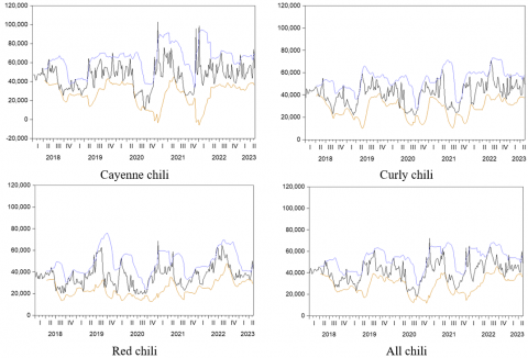
Visually, the weekly average price fluctuations of chili peppers in the primary market of Bandung City (the capital of West Java Province) are presented in Figure 2. It appears that, in general, during the period, the price trend was relatively mild, but highly volatile.
Figure 2. Weekly price volatility of chili in Pasar Induk Bandung, 2018 – May 2023
Table 3. Average weekly price of chili, lower and upper bands prices in grocer and farm gate markets (Rp/Kg)
|
Chili Type |
Summary Stats |
Grocer Market |
Farm Gate *) |
|||||
|
Mean |
Std. Dev. |
Min |
Max |
<ll |
> ul |
< ll |
> ul |
|
|
Cayenne chili |
45761 |
13989 |
10275 |
102719 |
7(2.6) |
15(5.6) |
37(13.9) |
4(1.5) |
|
Curly chili |
41109 |
10055 |
21669 |
70668 |
4(1.5) |
16(6.0) |
44(16.5) |
0(0.0) |
|
Red chili |
36413 |
10303 |
19471 |
68610 |
5(1.9) |
20(7.5) |
35(13.2) |
1(0.4 |
|
All |
41094 |
9960 |
18269 |
72186 |
4(1.5) |
17(6.4) |
68(25.6) |
2(0.8) |
Note: ll =lower level bands; ul=upper level bands
*) The comparison between farm gate prices and market prices is based on information obtained from FGDs involving chili farmers and traders.
Related to its characteristics, different types of chilies imply price fluctuations. Some studies also reported the similar phenomena [58]. The volatility of chili prices by chili type and market (grocer market and farm gate market) is shown in Table 3. Column 6 and column 7 are the frequency of actual prices in the wholesale market reaching the upper and lower Bollinger bands. Column 8 and column 9 are the frequency of actual prices at the Farm gate reaching the upper and lower Bollinger bands. The numbers in parentheses indicate the percentage of occurrence of upper and lower bands to the total number of weeks of observation (266 weeks). Referring to the information obtained in the FGDs, the farm gate price level for cayenne =85%, curly chili =89%, and red chili =88% when compared to the price in the grocer market. The "all" chili price is the average price of cayenne, curly and red chili. Since the farm gate price is obtained from this approach, the figures for the farm gate column in Table 3 are indicative, because empirically the difference between the price at the grocer market and the price at the farm gate level varies over time.
Price fluctuations 2018 – 2023 (second week of May) in 'Pasar Induk" (grocer market) show four lower band and 17 upper band experiences for all types of chilies. Lower bands occur from June to September and February, while the upper bands move more evenly from April to September and December to January. In the month when chili price fluctuations reach the lower bands, it generally occurs during the harvest season, which varies by region depending on the time of the planting season. When chili prices get the upper bands, it occurs typically at particular moments and holidays, and outside the harvest season.
With price transmission, the lower and upper levels of Bollinger can actually be used as a reference for price range expectations. But in contrast to the price in the grocer market, the price at the farm gate experiences more frequent fluctuations that tend to lower levels. For all chili, the lower level occurred 35 times, or about 13.2% of the total 266 weeks of observation. However, it only encountered one upper level. This indicates that price reductions to the lower level occur to farmers more frequently than price increases to the upper level.
The phenomenon of price volatility at the farm gate, which tends to move towards lower levels, is opposite to the phenomenon of price volatility in the grocer market, which tends to move to upper levels. Price movements to upper levels in the grocer market are not fully transmitted to prices at the farm gate level. Farmers more often receive low price fluctuations towards the lower level. Differentiated by chili type (cayenne chili, curly chili, and red chili), the volatility of chili prices both in the grocer market and farm gate shows the same pattern as the volatility pattern of all chili peppers (Table 3).
Differentiated by type of chili, on average, the price of cayenne chili per kg during the observation period was the highest compared to curly chili and red chili. The standard deviation shows that the cayenne chili price has the highest price risk. Figure 2 shows the prices of cayenne chili are very volatile. The price gap between the lower and upper bands is vast. Compare to other chilies, cayenne chili price is more volatile. The volatility of chili prices, especially cayenne chili, can be analyzed from the production side and the consumption side. From the supply side, there is a high disparity across regions. At the aggregate level, the majority of the cayenne chili area (around 61%) is only in four provinces out of 34 provinces in Indonesia in 2022, namely Central Java, West Java, East Java and DKI Jakarta. Any disruption in chili production in one or more key regions may lead to a significant impact on national supply and prices. This interplay of regional production capacities and challenges directly contributes to the volatility of chili prices on a national scale. In a smaller scope, this condition will have an impact on price fluctuations at the provincial level. For red and curly chili, production disparities between regions are relatively lower. From the consumption perspective, the elasticity of substitution for red versus curly chili is greater than for cayenne versus red chili, which explain why red and curly chilies are relatively stable in consumption. In addition, household participation rate and per capita consumption of cayenne chili are higher than red chili, influencing the degree of price fluctuations following production shocks. The dynamics between consumption patterns and production levels play crucial roles in determining price volatility.
The higher price volatility of cayenne chili compared to red chili is also shown by the study [59] from January 2017 to March 2018. The other research showed that the high volatility of red chili prices [60]. The study by Nugrahapsari and Arsanti [6] showed the price volatility of curly chili is relatively lower than that of cayenne chili, while the survey [61] showed that the price volatility of curly red chili at the producer and wholesale levels was relatively high.
The correlation between red chili and curly chili prices (0.73) is higher than between red chili and cayenne chili (0.55). The high correlation between red and curly chili prices indicates that the two commodities have similar price movements over time. The similarity is possible because red and curly chili are substitute to each other as cooking spices. In contrast, cayenne chili cannot substitute red or curly chili completely in its function as a spice. The high positive correlation between prices of the two commodities can significantly affect farmers' decisions regarding crop diversification. If the two commodities are highly positively correlated in terms of price movements, diversification into both crops may not effectively spread the risk because both crops are likely to be affected similarly by market conditions. Therefore, red and curly chilies farmers discourage to do crop diversifications. In contrast, low correlations between the prices of cayenne and red chili can encourage farmers to diversify their crop production to reduce the impact of price volatility and other risks on farm income.
Price fluctuations of each type of chili show a cyclical pattern consistent with the overall chili pattern, i.e., high prices occur from December to May of the following year. In these months, price fluctuations lead to high prices, while in June to November, the price changes lead to low prices. These results, consistent with the analysis by Lestari et al. [5], show that red chili price volatility occurs at the beginning, middle, and end of the year.
The question is, to what extent do farmers consider these price fluctuations with planting schedules to obtain more favorable price opportunities? From the monthly price during the observation period (January 2018 - May 2023), it was found that high chili prices occurred from December to May of the following year. High prices in these months could be due to high demand that exceeds the regular average supply or, conversely, reduced supply because it coincides with the planting season.
There are several notable moments and holidays in Indonesia where the demand for foodstuffs, including chili, increases, thus pushing up prices. First, the one-month Fasting Month (Ramadhan) for Muslims is until Eid Mubarak Day, which, during the observation period (January 2018 to May 2023), is between April, May, or June. Second, the Eid Al-Adha Mubarak takes place about 70 days after Eid Mubarak Day, around July, August, or September. Although Eid Al-Adha Mubarak is only one day, the celebration can last for four days. Third, the Christmas celebration in December. Fourth, the New Year celebration in January. Fifth, other memorable holidays and the months of the chili off-season. On these holidays, there are generally changes in people's consumption patterns, and they tend to cook a variety of dishes with chili ingredients. This yearly occurrence raises the demand for and price of chilies. The research indicates that there is a considerable positive influence on the variation of chili prices due to the specific holidays in Indonesia, which are expressed as dummy variables., i.e., for cayenne chili (α = 0.01), curly red chili (α = 0.01) and red chili (α = 0.05).
By considering the harvest period of chili, which is about 3.5 - 4 months after planting for the monoculture pattern or 4.5 months for the polyculture pattern, to have the opportunity for high prices that are more profitable, farmers will plant chili around August - November. However, it is not guaranteed that farmers will be able to capitalize on the momentum of price gains. Farmers must also consider the management of other crops and their off-farm activities. In fact, December to May is the rainy season, which is generally the planting season for farmers to utilize rainwater for their farming. The harvest season will last for 2-6 months, depending on the type of chili. For cayenne chili, the harvest period can continue for 4-6 months.
Consideration of planting and harvesting periods, to obtain more profitable high-price opportunities is supported by plot distribution of chili planting by month (Table 4). It shows that the most significant percentage of chili plots were planted from November to January, in the range of 11% -15%, compared to other months, which were only around 1% -8%. Meanwhile, the distribution of plots by harvest month shows the dominant percentage of plots is in December, February-March, and June-July, reaching a range of 11%-19%.
Table 4. Plots distribution of chili by planting and harvest month
|
Month |
∑Plots Planting (%) |
∑Plots Harvesting (%) |
|
January |
15.19 |
2.53 |
|
February |
11.39 |
12.66 |
|
March |
3.8 |
13.92 |
|
April |
1.27 |
7.59 |
|
May |
3.8 |
7.59 |
|
June |
3.8 |
18.99 |
|
July |
11.39 |
17.72 |
|
August |
5.06 |
5.06 |
|
September |
7.59 |
11.39 |
|
October |
8.86 |
2.53 |
|
November |
13.92 |
2.53 |
|
December |
15.19 |
12.66 |
Chili farming is confronted with a substantial risk due to the extreme price volatility. Farmers experience price decreases more often at the lower level than price increases at the upper level. However, farmers are motivated to grow chili as it has more significant profit than other vegetable farming. Factors conducive to increasing farmers' chances of participation in chili farming are increased access to market price volatility, the role of farming in household income, and positive attitudes towards the role of vegetables as a way to increase income. Farmers with younger age have a higher chance and intensity to participate. Particularly for those who participate, if their risk aversion is lower, the motive to scale up increases. Other factors that are conducive to scale-up are experience in farming, availability of family labor, and ability to access information on price volatility and self-financing.
Effective policies to increase farmers' income and chili price stability include the following. First, the coordination system of farmers in planning chili planting patterns and schedules should be strengthened so that the variation in supply over times can be reduced. Second, increasing farmers' access to market information, so that price volatility can be anticipated. Third, improving the ability of farmers to finance their farms through increased access to formal credit services. Fourth, promote policies related to the creation and dissemination of chili cultivation technologies that are labor-saving, productivity enhancing, and adaptive to environmental stresses related to climatic conditions.
To stabilize chili prices in the optimal price range and to help mitigate the impact of price volatility, a combination of strategies is needed related to various factors, such as weather conditions, market demand, and agricultural practices, as the following. First, weather risk management through utilizing greenhouse farming or investing in irrigation systems. Second, providing farmers with timely and accurately market information on when to sell during price downturns, Third, research and technology through investing in research for more resilient chili varieties, better farming techniques, and pest management. Forth, government intervention on price stabilization funds, or price controls to stabilize prices within a specific range.
[1] Sativa, M., Harianto, H., Suryana, A. (2017). Impact of red chilli reference price policy in Indonesia. International Journal of Agriculture System, 5(2): 120-139. https://doi.org/10.20956/ijas.v5i2.1201
[2] Lukas, A., Kairupan, A.N., Hendriadi, A., et al. (2023). Fresh chili agribusiness: Opportunities and problems in Indonesia. Agricultural Economics and Agri-Food Business. https://doi.org/10.5772/intechopen.112786
[3] Statistik Hortikultura Provinsi DKI Jakarta 2022. https://jakarta.bps.go.id/publication/2023/10/17/b5c448710fa9debc90c9955b/statistik-hortikultura-provinsi-dki-jakarta-2022.html, accessed on Mar. 23, 2024.
[4] Nasruddin, W., Musyadar, A., Gandasari, D. (2019). Perilaku petani cabai merah dalam perencanaan pemasaran di sentra produksi Jawa Barat, Indonesia. Jurnal Agroekoteknologi dan Agribisnis, 3(2): 37-45.
[5] Lestari, E.P., Prajanti, S.D.W., Wibawanto, W., Adzim, F. (2022). ARCH-GARCH analysis: An approach to determine the price volatility of red chili. AGRARIS: Journal of Agribusiness and Rural Development Research, 8(1): 90-105. https://doi.org/10.18196/agraris.v8i1.12060
[6] Nugrahapsari, R.A., Arsanti, I.W. (2018). Analisis volatilitas harga cabai keriting di Indonesia dengan pendekatan ARCH GARCH. Jurnal Agro Ekonomi, 36(1): 25-37. https://doi.org/10.21082/jae.v36n1.2018.25-37
[7] Viana, C.D.N., Hartono, S., Waluyati, L.R. (2017). Volatility analysis on producer price of red pepper and cayenne pepper in west Java Province Indonesia. Agro Ekonomi, 28(2): 157-169. https://doi.org/10.22146/jae.25939
[8] BI-Indonesia. (2018). Kajian ekonomi dan Keuangan Regional, Bank Indonesia, 13(4). https://www.bi.go.id/id/publikasi/laporan/Documents/Laporan%20Nusantara%20November%202018.pdf.
[9] Wibowo, H.E., Novanda, R.R., Khaliqi, M., Sinaga, F.H., Darmansyah, D., Amiruddin, A., Sari, I.R.M. (2023). Volatility analysis of chili price at Bengkulu Province using ARIMA approach. IOP Conference Series: Earth and Environmental Science, 1230(1): 012013. https://doi.org/10.1088/1755-1315/1230/1/012013
[10] Webb, A.J., Kosasih, I.A. (2011). Analysis of price volatility in the Indonesia fresh chili market. In Annual Meeting of the International Agricultural Trade Research Consortium, USA, pp. 11-13.
[11] Analisis Inflasi Mei 2023 Jakarta. https://www.bi.go.id/id/publikasi/ruang-media/news-release/Pages/sp_2515023.aspx, accessed on Apr. 2, 2024.
[12] Preciosa, Y.N., Sariyoga, S., Sari, R.M. (2019). Dampak kebijakan penetapan harga acuan terhadap volatilitas harga cabai besar di Indonesia. Jurnal Agribisnis Terpadu, 12(1): 59-71.
[13] Muflikh, Y.N., Smith, C., Brown, C., Aziz, A.A. (2021). Analysing price volatility in agricultural value chains using systems thinking: A case study of the Indonesian chilli value chain. Agricultural Systems, 192: 103179. https://doi.org/10.1016/j.agsy.2021.103179
[14] Dewi, H.A., Daroini, P.B., Ndaru, R., Negoro, A.A., Latifah, E. (2021). Analysis of agribusiness performance of top five vegetable farming in East Java. IOP Conference Series: Earth and Environmental Science, 892(1): 012003. https://doi.org/10.1088/1755-1315/892/1/012003
[15] Halid, A., Murtisari, A., Abuya, I. (2014). Analisis perbandingan usahatani cabai rawit dan tomat dengan pendekatan resiko investasi di desa tolite jaya kecamatan tolinggula kabupaten gorontalo utara. Jurnal Perspektif Pembiayaan dan Pembangunan Daerah, 1(4): 191-191. https://doi.org/10.22437/ppd.v1i4.1710
[16] Sembiring, C.Y.B., Waluyati, L.R. (2021). The analysis of cost structure, income, and profitability for horticulture farming on coastal sand area In Bugel Village, Panjatan District, Kulon Progo Regency. Journal of Agribusiness Management and Development, 2(1): 105-111.
[17] Eliyatiningsih, E., Mayasari, F. (2018). Factors that influence farmer decision to keep his red chili farming in Wuluhan District, Jember Regency. In Proceeding of the 1st International Conference on Food and Agriculture.
[18] Garcia-Yi, J. (2014). Market participation and agro-biodiversity loss: The case of native chili varieties in the Amazon rainforest of Peru. Sustainability, 6(2): 615-630. https://doi.org/10.3390/su6020615
[19] Mariyono, J., Sumarno, S. (2015). Chilli production and adoption of chilli-based agribusiness in Indonesia. Journal of Agribusiness in Developing and Emerging Economies, 5(1): 57-75.
[20] Cragg, J.G. (1971). Some statistical models for limited dependent variables with application to the demand for durable goods. Econometrica: Journal of the Econometric Society, 829-844.
[21] García, B. (2013). Implementation of a double-hurdle model. The Stata Journal, 13(4): 776-794. https://doi.org/10.1177/1536867X1301300406
[22] Engel, C., Moffatt, P.G. (2014). dhreg, xtdhreg, and bootdhreg: Commands to implement double-hurdle regression. The Stata Journal, 14(4): 778-797. https://doi.org/10.1177/1536867X1401400405
[23] Assouto, A. B., Houensou, D. A. and Semedo, G. (2020) ‘Price risk and farmers’ decisions: A case study from Benin’, Scientific African, 8(March), pp. 1-11. https://doi.org/10.1016/j.sciaf.2020.e00311
[24] Tropea, F. (2016). Price volatility in agricultural markets: Risk management and other tools. EPRS: European Parliamentary Research Service.
[25] Apergis, N., Rezitis, A. (2003). Agricultural price volatility spillover effects: The case of Greece. European Review of Agricultural Economics, 30(3): 389-406. https://doi.org/10.1093/erae/30.3.389
[26] Gilbert, C.L., Morgan, C.W. (2010). Food price volatility. Philosophical Transactions of the Royal Society B: Biological Sciences, 365(1554): 3023-3034. https://doi.org/10.1098/rstb.2010.0139
[27] Manogna, R.L., Mishra, A.K. (2020). Price discovery and volatility spillover: An empirical evidence from spot and futures agricultural commodity markets in India. Journal of Agribusiness in Developing and Emerging Economies, 10(4): 447-473. https://doi.org/10.1108/JADEE-10-2019-0175
[28] Barbaglia, L., Croux, C., Wilms, I. (2020). Volatility spillovers in commodity markets: A large t-vector autoregressive approach. Energy Economics, 85: 104555. https://doi.org/10.1016/j.eneco.2019.104555
[29] Thiyagarajan, S., Naresh, G., Mahalakshmic, S. (2015). Forecasting volatility in Indian agri-commodities market. Global Business and Finance Review, 20(1): 95-104. https://doi.org/10.17549/gbfr.2015.20.1.95%0A
[30] Wangu, J., Mangnus, E., van Westen, A.C.M. (2020). Limitations of inclusive agribusiness in contributing to food and nutrition security in a smallholder community. A case of mango initiative in Makueni county, Kenya. Sustainability, 12(14): 5521. https://doi.org/10.3390/su12145521
[31] Yip, P.S., Brooks, R., Do, H.X., Nguyen, D.K. (2020). Dynamic volatility spillover effects between oil and agricultural products. International Review of Financial Analysis, 69: 101465. https://doi.org/10.1016/j.irfa.2020.101465
[32] Mensi, W., Tiwari, A., Bouri, E., Roubaud, D., Al-Yahyaee, K.H. (2017). The dependence structure across oil, wheat, and corn: A wavelet-based copula approach using implied volatility indexes. Energy Economics, 66: 122-139. https://doi.org/10.1016/j.eneco.2017.06.007
[33] Haixia, W., Shiping, L. (2013). Volatility spillovers in China’s crude oil, corn and fuel ethanol markets. Energy Policy, 62: 878-886. https://doi.org/10.1016/j.enpol.2013.07.026
[34] Rogers, W. (1994). Regression standard errors in clustered samples. Stata Technical Bulletin, 3(13).
[35] Cameron, A.C., Miller, D.L. (2010). Robust inference with clustered data. In: Handbook of Empirical Economics and Finance, 106: 1-28.
[36] Wooldridge, J.M. (2003). Cluster-sample methods in applied econometrics. American Economic Review, 93(2): 133-138. https://doi.org/10.1257/000282803321946930
[37] Van Phan, P., O'Brien, M. (2022). Is small beautiful? An empirical analysis of land characteristics and rural household income in Vietnam. Australian Journal of Agricultural and Resource Economics, 66(3): 561-580. https://doi.org/10.1111/1467-8489.12476
[38] Twumasi, M.A., Jiang, Y., Acheampong, M.O. (2019). Determinants of agriculture participation among tertiary institution youths in Ghana. Journal of Agricultural Extension and Rural Development, 11(3): 56-66. https://doi.org/10.5897/JAERD2018.1011
[39] Susilowati, S.H., Perdana, R.P., Sudaryanto, T., Agustian, A. (2023). Profit variability of vegetable farming in the upper Citarum watershed, West Java, Indonesia. IOP Conference Series: Earth and Environmental Science, 1230(1): 012193. https://doi.org/10.1088/1755-1315/1230/1/012193
[40] Mailena, L., Indrawanto, C., Astuti, E.P. (2021). Risk management of chilli supply chains using weighted failure mode effect analysis. IOP Conference Series: Earth and Environmental Science, 782(2): 0220040. https://doi.org/10.1088/1755-1315/782/2/022004
[41] Kering, I.P.L. (2019). Adaptasi tanaman hortikultura terhadap perubahan. Jurnal Litbang Pertanian, 38(1): 55-64. https://doi.org/10.21082/jp3.v38n1.2019.p55-64
[42] Amira, F., Andina, M., Sasmita, S. (2021). Analisis faktor-faktor yang mempengaruhi keputusan petani dalam melakukan usahatani cabai rawit (studi kasus di desa bungatan kecamatan bungatan kabupaten situbondo). Agribios, 19(2): 89-95.
[43] Marveldani, M., Maulana, E., Maulida, D. (2018). Evaluasi daya hasil lima varietas cabai (Capsicum annuum L.) dengan penggunaan mulsa plastik dan paranet saat transplanting. In Prosiding Seminar Nasional Pengembangan Teknologi Pertanian. https://doi.org/10.25181/prosemnas.v2018i0.1175
[44] Mustamu, N.E. (2014). Respon pertumbuhan dan produksi tanaman cabai keriting (Capsicum annuum l.) terhadap pemberian pupuk NPK 16-16-16 Dan Pupuk Kandang Lembu. Jurnal Agroplasma, 1(1). https://doi.org/10.36987/agr.v1i1.121
[45] Kumaat, R.M., Katiandagho, T.M. (2021). Motivasi petani dalam budidaya tanaman cabai di desa raanan baru kecamatan motoling barat kabupaten minahasa selatan. AGRI-SOSIOEKONOMI, 17(2): 303-312. https://doi.org/10.35791/agrsosek.17.2.2021.33837
[46] Sahara, S., Minot, N., Stringer, R., Umberger, W.J. (2015). Determinants and effects of small chilli farmers’ participation in supermarket channels in Indonesia. Bulletin of Indonesian Economic Studies, 51(3): 445-460. https://doi.org/10.1080/00074918.2015.1110851
[47] He, Z., Weng, H., Ho, H.C., Ran, Q., Mao, M. (2014). Soil erosion and pollutant transport during rainfall-runoff processes. Water Resources, 41: 604-611. https://doi.org/10.1134/S0097807814050170
[48] Muoni, T., Koomson, E., Öborn, I., Marohn, C., Watson, C. A., Bergkvist, G., Barnes, A., Cadisch, G., Duncan, A. (2020). Reducing soil erosion in smallholder farming systems in east Africa through the introduction of different crop types. Experimental Agriculture, 56(2): 183-195. https://doi.org/10.1017/S0014479719000280
[49] Prancevic, J.P., Lamb, M.P., McArdell, B.W., Rickli, C., Kirchner, J.W. (2020). Decreasing landslide erosion on steeper slopes in soil‐mantled landscapes. Geophysical Research Letters, 47(10): e2020GL087505. https://doi.org/10.1029/2020GL087505
[50] Jumiyati, S., Arsyad, M., Hadid, A., Toknok, B., Sjamsir, Z. (2020). Implementation of environmental-economic concepts through farming risk management in highland vegetable agroforestry. IOP Conference Series: Earth and Environmental Science, 575(1): 012061. https://doi.org/10.1088/1755-1315/575/1/012061
[51] Aerts, R., Hundera, K., Berecha, G., Gijbels, P., Baeten, M., Van Mechelen, M., Hermy, M., Muys, B., Honnay, O. (2011). Semi-forest coffee cultivation and the conservation of Ethiopian Afromontane rainforest fragments. Forest Ecology and Management, 261(6): 1034-1041. https://doi.org/10.1016/j.foreco.2010.12.025
[52] Pinard, F., Joetzjer, E., Kindt, R., Kehlenbeck, K. (2014). Are coffee agroforestry systems suitable for circa situm conservation of indigenous trees? A case study from Central Kenya. Biodiversity and Conservation, 23: 467-495. https://doi.org/10.1007/s10531-013-0615-0
[53] Negawo, W.J., Beyene, D.N. (2017). The role of coffee based agroforestry system in tree diversity conservation in Eastern Uganda. Journal of Landscape Ecology, 10(2): 1-18. https://doi.org/10.1515/jlecol-2017-0001
[54] Valencia, V., West, P., Sterling, E.J., García-Barrios, L., Naeem, S. (2015). The use of farmers' knowledge in coffee agroforestry management: Implications for the conservation of tree biodiversity. Ecosphere, 6(7): 1-17. https://doi.org/10.1890/ES14-00428.1
[55] Zamora, A.G., Rodríguez, M.E., Barradas, V.L. (2016). Mountain cloud forest and grown-shade coffee plantations: A comparison of tree biodiversity in central Veracruz, Mexico. Forest Systems, 25(1): 10.
[56] Wardhono, A., Nasir, M.A., Qori’ah, C.G., Indrawati, Y. (2021). Perfecting policies of chili agribusiness to support food security: Evidence from Indonesia districts. IOP Conference Series: Earth and Environmental Science, 759(1): 012048. https://doi.org/10.1088/1755-1315/759/1/012048
[57] Sánchez Toledano, B.I., Camarena Gómez, D.M.J., López Santiago, M.A., Cuevas Reyes, V. (2023). Consumer preferences of jalapeño pepper in the Mexican market. Horticulturae, 9(6): 684. https://doi.org/10.3390/horticulturae9060684
[58] Ponnaluru, S. S. (2020). Spatial hedonic price analysis of dry chillies in Karnataka. The Journal of Research ANGRAU, 48(3): 110-115.
[59] Wardhono, A., Indrawati, Y., Qori’ah, C.G., Nasir, M.A. (2020). Institutional arrangement for food price stabilization and market distribution system: study of chili commodity in Banyuwangi regency. In E3S Web of Conferences, 142: 05006. https://doi.org/10.1051/e3sconf/202014205006
[60] Putri, H., Cahyani, P.C. (2016). Price volatility of main food commodity in Banyumas Regency Indonesia. International Journal on Advanced Science, Engineering and Information Technology, 6(3): 374-377.
[61] Sukiyono, K., Asriani, P.S. (2020). Volatilitas dan transmisi harga cabai merah keriting pada pasar vertikal di Provinsi Bengkulu. Jurnal Agro Ekonomi, 38(1): 29-39.