Bedr-Eddine Benaissa | Chahrazed Bessenouci | Omolayo M. Ikumapayi![]() | Ayad Q. Al-Dujaili
| Ayad Q. Al-Dujaili![]() | Ahmed I. Abdulkareem | Amjad J. Humaidi
| Ahmed I. Abdulkareem | Amjad J. Humaidi![]() | Giulio Lorenzini
| Giulio Lorenzini![]() | Younes Menni*
| Younes Menni*![]()
© 2023 IIETA. This article is published by IIETA and is licensed under the CC BY 4.0 license (http://creativecommons.org/licenses/by/4.0/).
OPEN ACCESS
Wireless sensor networks (WSNs) are attracting great interest from a large research community. The main function of these types of networks is their ability to collect physical data from a given environment such as temperature, humidity and light, etc. They are mainly designed for low-power embedded communications. One of the most felt drawbacks of sensor nodes is their inability to recognize their own positions if they are not equipped with a global positioning module (GPS). In this paper, we first implemented the traditional "Distance Vector Hop" localization algorithm, known by the acronym "DV-Hop", on the Cooja/Contiki platform, which served as a control sample. Subsequently, we developed a new contribution in which the unknown node estimated its distance to all anchors in the network, based only on locally available information. Our goal was to significantly reduce the distance gap between the actual and the estimated distance. The idea of the contribution was implemented on the Cooja/Contiki emulator, and was based on two techniques: 1- Calculating the distance error rate (Euclidean distance/SSRI distance). 2- Converting the type of node once located into an anchor. Our simulation results show that the proposed DVA-Hop algorithm had a better accuracy than the native "DV-Hop" method.
wireless sensor network (WSN), DV-Hop, localization node, received signal strength indicator (RSSI)
Among the most coveted areas in artificial intelligence in the last decade have been deep learning and sensor networks for remote monitoring and control. This major interest in data collection and manipulation has allowed sensor networks to take a prominent place in many applications such as surveillance, home automation and human activity. We attach great importance to the deployment of sensors and their positioning, as a large event can lead to an unrepairable disaster. So, the location of the "event triggering" sensor must signal its position to the data sink so as it can be responded to in record time. Thus, several improved researches have been elaborated revealing effective results and suggesting recommendations for deployment [1]. Localisation consists in knowing the physical position of nodes within the network in order to give value to the interpretations of the collected data.
Several application areas rely on localisation systems:
-Wildlife monitoring,
-Home automation,
-Industrial control and,
-Permanent monitoring.
Many researchers have addressed this issue by proposing localisation heuristics [2, 3], based as a whole, on special known nodes called "anchors" that are equipped with GPS that know their positions. The importance of a localisation system is that it allows us to sort out where the measurements were taken by the event capture system.
Furthermore, the availability of location information would allow for the emergence of other application areas in the future. The cost of a sensor network plays an important role too. In this perspective, one cannot afford to deploy only sensors with an integrated GPS positioning module [4]. Thus, the task of building an efficient and cost-effective network becomes very difficult.
Nevertheless, a number of researchers have tackled this issue, and have proposed location algorithms and/or heuristics that are reliable enough. They were divided into two categories: the first called "Range Based" which identifies the location of unknown nodes based on the distance and theangle between the anchor nodes, and then announces their position by triangulation, i.e., the most credible three-way approximation. The strength of this technique lies in the accuracy of locating lost nodes, but the high resource cost and the difficult deployment make their uses rather reduced. Among these algorithms, we have DV-Distance, DV-Euclidean, etc. The second category, "Range Free", is based on information about the radio range and the hops between nodes. Note that the "Range Free" approaches have become very successful thanks to the following algorithms: DV-hop, Centroid, Amorphous, APIT, DV-Hop Max and the SPA algorithm [5, 6].
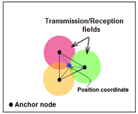
New geometric techniques have emerged to complement the previous two. Known as "distance combination": Multilateration, trilateration and triangulation provide more precision in the position of the node. These techniques are widely used in the universal GPS position calculation system. Important applications (military, environmental, domestic, and medical, etc.) use wireless sensors and rely on their random deployments which require precise localisation of their positions in a fixed coordinate system. The issues highlighted in localisation are mainly: routing, quality of service, security and mobility. Various techniques exploit connectivity information as an aid to find unknown nodes and estimate their distances in a randomly distributed topology. One such method is the Distance Vector-Hop algorithm (DV-Hop). In this paper, we will explain the DV-Hop algorithm, and present some recent research that has studied and improved it, and then propose a contribution in the same context. A location system generates three components (see Figure 1):
-A distance/angle estimation system.
-A method for calculating the position.
-A localisation algorithm.
Figure 1. Location system: Triangulation
The accuracy of node locations is one of the most coveted problems in localisation, especially as an internal environment does not have the same constraints as the external one. It is in this perspective that an unknown point must inevitably have an indication beacon, often called an anchor.
It should be noted that the most commonly used jump algorithm in the context of localisation is the "DV-hop" because of its simplicity, as it is based on the number of jumps between the anchor node (whose geographical position is known) and the unknown node. DV-hop requires at least three anchor nodes for its animation. These anchors regularly transmit their coordinates to their neighbors, which in turn transmit them to the other nodes, generating various heuristics. Many studies have been inspired by this algorithm, as it offers autonomous localisation of all deployed sensors.
The rest of this paper (section 2) shows the DV-Hop method to highlight the shortcomings of this algorithm. An overview of related research work is presented in section 3 and an attempt to propose our contribution in section 4. Interpretation of the experimental results and a conclusion follow.
2.1 Understanding the DV-hop algorithm
"DV-Hop" was cited by Niculescu et al. [7]. It is a distributed location algorithm based on a distance routing protocol. In its design, it relies on three phases to estimate the hop distance between the unknown node and the anchor nodes. But this estimation creates errors, especially in the calculation of the average hop size of each anchor [8]. In order to correct its location accuracy, many modifications and improvements have been made to the basic DV-Hop. The first phase calculates the minimum number of hops between all sensor nodes. In the second phase, the average hop size is estimated and the distance between the nodes is calculated. The third phase calculates the position of the unknown node using a latency method [9].
1st phase: Approximation of the optimal number of jumps.
During this phase, each anchor begins to flood the network with its format packet:
"PAi = [idBeacon, (xAi, yAi), hopAi]", in order to announce its position at a time "t":
- PAi: Anchor-specific package
- idBeacon: Beacon identifier.
- (xAi, yAi): Coordinates of the ith anchor.
- hopAi: Number of hops from the anchor node, initially set to zero.
Each node of the network {S1, S2, S3, U?, ...} receiving a packet {PAi}, from any anchor node "Ai", at time "t", is instantaneously compared to the previously received packet {PAi-1} of time "t-1". If the number of hops {hopAi} is greater than the number of hops of the received packet {hopAi-1}, then the packet is ignored by the said node. Otherwise, it will update its hop table by adding a hop in the {hopAi} field of the packet and then rebroadcast this updated packet on the network. Each unknown node stores the packet {PAi} with the minimum number of hops received from each anchor node.
2nd phase: Determination of the average jump size between the anchors.
Each anchor estimates the average hop size with respect to all anchor nodes in the network, using Eq. (1) as specified below:
${ }^1 H o p_{\text {average }}\left(A_{i j}\right)=\frac{\sum_{i \neq j}^k \sqrt{\left(x_i-x_j\right)^2+\left(y_i-y_j\right)^2}}{\sum_{i \neq j}^k \operatorname{hop}_{A i j}}$ (1)
where,
(xi, yi): Coordinates of the ith anchor node.
(xj, yj): Coordinates of the jth anchor node.
hopAij: Minimum number of hops from the anchor node {i} to the anchor node {j}.
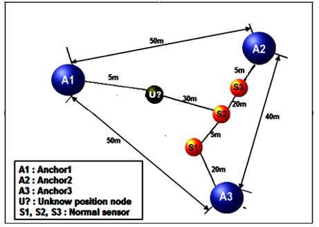
Note: the anchor node {j} represents all other anchor nodes that are different (≠) from the anchor node {i}. Consider the example in Figure 2.
Figure 2. Example of the application of the DV-hop algorithm
The anchor nodes {A1, A2 and A3} know their positions. In this case, we calculate the Euclidean distance of A1A2; A1A3; A2A3, using Eq. (1), the results are highlighted in Table 1.
Table 1. Distance and number of hops between anchor nodes
|
Path according to Figure 2. |
A1-A2 |
A1 A3 |
A2-A3 |
|
Actual distance (metres) |
50m |
50m |
40m |
|
Number of jumps=Path Ai$\rightarrow$Aj |
4 |
4 |
4 |
The calculated average jump sizes of the anchors {A1, A2 and A3} are shown in Figure 2. For example, the Euclidean distance of {A1} has both a Euclidean distance to {A2} and also to {A3} of length 4 hops, so we will get a correction of the estimated average hop size of each of the anchors by applying Eq. (1). Note that the anchor node {A1} has the choice of either calculating a single correction to be broadcast in the network, or sending considerably different corrections in different directions. In our experiments, we use the first option. For example:
- Path A1-A2: A1$\rightarrow$ U? $\rightarrow$ S2$\rightarrow$ S3$\rightarrow$ A2 = 4 jumps.
- Path A1-A3: A1$\rightarrow$ U? $\rightarrow$ S2$\rightarrow$ S1$\rightarrow$ A3 = 4 jumps.
- Path A2-A3: A1$\rightarrow$ S 3$\rightarrow$ S2$\rightarrow$ S1$\rightarrow$ A2 = 4 jumps.
Thus, the average size of a hop at the anchor {A1} noted: 1hopaverage {A1} is:
$\begin{gathered}{ }^1 \operatorname{Hop}_{\text {average }}\left(A_1\right)=\frac{\operatorname{Dist}\left(A_1 A_2\right)+\operatorname{Dist}\left(A_1 A_3\right)}{\operatorname{hop}\left(A_1 A_2\right)+\operatorname{hop}\left(A_1 A_3\right)} \\ =\frac{50+50}{4+4}=12.5 \mathrm{~m}\end{gathered}$
And possibly for $\left\{A_2\right\},\left\{A_3\right\}$ :
${ }^1 \mathrm{Hop}$ average $\left(A_2\right)=\frac{50+40}{4+4}$
${ }^1 H o p_{\text {average }}\left(A_3\right)=\frac{50+40}{(4+4)}=11.25 \mathrm{~m}$
Using Eq. (1), the anchor nodes calculate each other's average one-hop distances between them. Once these magnitudes are calculated $\left\{{ }^1 \operatorname{hop}_{\text {average }}(A i)\right\}$, the anchors broadcast these values over the network. As a result, each unknown node $\left\{U ?_{\mathrm{m}}\right\}$ can calculate its distance to the nearest anchor $\left\{A_i\right\}$ by applying Eq. (2).
$U ?^{\text {dist }}\left(A_m\right)$=${ }^1$ hop $_{\text {average }}\left(A_m\right) \times$ hop $_{A m}$ (2)
-U? ${ }^{\text {dist }}\left(\mathrm{A}_{\mathrm{m}}\right)$ : Distance between the anchor node $\{A i\}$ and the unknown node $\left\{U ?_{\mathrm{m}}\right\}$.
- ${ }^1$ hop average $\left(A_m\right)$: Average size of a jump between anchor {i} and anchor {m}.
- $h_{h o p}{ }_{A m}$: Total number of hops from the anchor node {i} to the anchor node {m}.
Let us observe this distance calculation on our example in Figure 2. Suppose that an unknown node {U?} gets its correction from the anchor {A2}. Thus, its average hop size is estimated to be: 1hopaverage{A2} = 11.25 m, and thus by applying Eq. (2), its distances are estimated then, relative to the three landmarks {A1}, {A2} and {A3} as follows:
$\begin{aligned} & -U ?^{\text {dist }}\left(A_1\right)=1 \times 11.25=11.25 \mathrm{~m} \\ & -U ?^{\text {dist }}\left(A_2\right)=3 \times 11.25=33.75 \mathrm{~m} \\ & -U ?^{\text {dist }}\left(A_3\right)=3 \times 11.25=33.75 \mathrm{~m}\end{aligned}$
Note: We notice that the value of the average distance of a jump is kept at the distance of the corrective anchor node, which in our case is {A2}.
Once these values have been calculated, they are then inserted into the triangulation procedure described by Eq. (3) in the next phase so that the unknown node {U?}, obtains an estimate of its geographical position (coordinates: CU?).
3rd phase: Determining the position of an unknown sensor {U?}
Only in this phase can the position of any sensor in the network be estimated. Here we calculate the position of the node {U?} using the distances estimated in the trilateration or Multilateration technique. Let us denote by (xu, yu), the coordinates of the unknown node {U?}, and by (xAn, yAn) the coordinates of the other anchor nodes {An}, and defining by "ƞA" the total number of anchors, and " $\mathrm{U} ?^{\text {dist }}\left(A_{\mathrm{i}}\right)$ " as the average distance of a hop from the anchor {Ai} estimated by Eq. (2).
The considered coordinates of the unknown sensor position {U?}, are obtained by Eq. (3) from the Global Positioning System (GPS) triangulation procedure [10], which we use in its simplified version as we only compute distances without taking into account the locking synchronisation. This procedure starts with an estimated location, a priori, which is then linearly corrected to an approximate real location.
$\left[\begin{array}{c}\left(x_U-x_{A 1}\right)^2+\left(y_U-y_{A 1}\right)^2=\left(U ?^{\text {dist }}\left(A_1\right)\right)^2 \\ \left(x_U-x_{A 2}\right)^2+\left(y_U-y_{A 2}\right)^2=\left(U ?^{\text {dist }}\left(A_2\right)\right)^2 \\ \vdots \\ \left(x_U-x_{A n}\right)^2+\left(y_U-y_{A n}\right)^2=\left(U ?^{\text {dist }}\left(A_n\right)\right)^2\end{array}\right]$ (3)
This last equation can also be expressed in the extended form, generating Eq. (4) below:
$\left[\begin{array}{c}x_{A 1}{ }^2-x_{A n}{ }^2+y_{A 1}{ }^2-y_{A n}{ }^2-\left(U ?^{\text {dist }}\left(A_1\right)\right)^2-\left(U ?^{\text {dist }}\left(A_{A n}\right)\right)^2=2 \cdot x_U \cdot\left(x_{A 1}-x_{A n}\right)+2 \cdot y_U \cdot\left(y_{A 1}-y_U\right) \\ x_{A 2}{ }^2-x_{A n}{ }^2+y_{A 2}{ }^2-y_{A n}{ }^2-\left(U ?^{\text {dist }}\left(A_2\right)\right)^2-\left(U ?^{\text {dist }}\left(A_{A n}\right)^2=2 \cdot x_U \cdot\left(x_{A 2}-x_{A n}\right)+2 \cdot y_U \cdot\left(y_{A 2}-y_U\right)\right. \\ \vdots \\ x_{A n-1}{ }^2-x_{A n}{ }^2+y_{A n}{ }^2-y_{A n-1}{ }^2-\left(U ?^{\text {dist }}\left(A_{n-1}\right)\right)^2-\left(U ?^{\text {dist }}\left(A_{A n}\right)\right)^2=2 \cdot x_U \cdot\left(x_{A n-1}-x_{A n}\right)+2 \cdot y_U \cdot\left(y_{A n-1}-y_U\right)\end{array}\right]$ (4)
With good observation, we present Eq. (4) in the form [A× CU? = B], where the variables of the matrix {A} are given by Eq. (5), {B} by Eq. (6), and that of the coordinates of the unknown node {CU?} are presented by Eq. (7).
$A=\left[\begin{array}{cc}2 \cdot\left(x_{A 1}-x_{A \mathrm{n}}\right) & 2 \cdot\left(y_{A 1}-y_U\right) \\ 2 \cdot\left(x_{A 2}-x_{A \mathrm{n}}\right) & 2 \cdot\left(y_{A 2}-y_U\right) \\ \vdots & \vdots \\ 2 \cdot\left(x_{A n-1}-x_{A n}\right) & 2 \cdot\left(y_{A n-1}-y_{U }\right)\end{array}\right]$ (5)
$B=\left[\begin{array}{c}x_{A 1}^2-x_{A n}^2+y_{A 1}^2-y_{A n}^2-\left(U ?^{\text {dist }}\left(A_1\right)\right)^2-\left(U ?^{\text {dist }}\left(A_{A n}\right)\right)^2 \\ x_{A 2}^2-x_{A n}^2+y_{A 2}^2-y_{A n}^2-\left(U ?^{\text {dist }}\left(A_2\right)\right)^2-\left(U ?^{\text {dist }}\left(A_{A n}\right)\right)^2 \\ \vdots \\ x_{A n-1}^2-x_{A n}^2+y_{A n}^2-y_{A n-1}^2-\left(U ?^{\text {dist }}\left(A_{n-1}\right)\right)^2-\left(U ?^{\text {dist }}\left(A_{A n}\right)\right)^2\end{array}\right]$ (6)
$C_{U ?}=\left[\begin{array}{l}x_{U ?} \\ y_{U ?}\end{array}\right]$ (7)
The estimate of the coordinates of the node {U?} is given by Eq. (8) below:
$C_{U ?}=\left(A^T \cdot A\right)^{-1} \cdot A^T \cdot B$ (8)
2.2 Standard DV-Hop localisation error
The basic algorithm of "DV-Hop" amplifies the error in calculating the position of the unknown node in two steps. One is in the process of selecting the minimum number of hops, and the other is in the calculation of the average distance of a hop. In this algorithm, all unknown nodes use the $\left\{{ }^1\right.$ hop average $\left.\left(\mathrm{A}_{\mathrm{m}}\right)\right\}$ to calculate the distance to the anchor nodes, following phase 2. It is assumed that all neighboring nodes are one hop away, regardless of their deployment in the real environment and this is one of the causes of the error. Illustrating this on our example in Figure 2, the unknown node {U?} is one hop away from the anchor node {A1} and the single node {S2}. While the average hop distance already calculated is:
-${ }^1$ hop average $\left\{A_1\right\}=12.50 \mathrm{~m}$,
-${ }^1$ hop average $\left\{A_2\right\}=11.25 \mathrm{~m}$,
-${ }^1$ hop $_{\text {average }}\left\{A_3\right\}=11.25 \mathrm{~m}$.
We notice that the reality is quite different, the real distance between the anchor {A1} and the unknown node is 5m instead of the estimated 12.50m. Therefore, the positioning error for {A1} is 7.5m = 12.50m - 5m. Thus, all unknown nodes use the average value of the nearest anchor jump, which will definitely impair the efficiency of the DV-Hop algorithm, as this error will be accumulated from one unknown node to another. Thus, the error increases and the accuracy is reduced.
In order to overcome this problem and to reduce the error rate as much as possible, several studies have been carried out to improve the efficiency of this algorithm. In the following section, a background of the latest contributions on localisation is presented in order to improve the standard DV-Hop algorithm.
One of the first algorithms to improve on the traditional DV-Hop is SDDV-HOP (Shortest Distances DV-HOP) by Hu et al. [11]. The latter proposes to modify the average hop distance of the network. The idea comes from the ratio between the shortest path distance and the straight distance between nodes. In graph theory, the shortest path problem is to find a path between two nodes in a graph so that the sum of the weights of its constituent edges is minimized. Another approach that slightly improves on this program is the work of the authors of [12], where they use a threshold "M" to manipulate weighted average hop distances of anchor nodes in the limit "Msauts" with unknown nodes, and other anchor nodes whose hop count is greater than "M" are ignored. Their results show that the optimal average positioning error results from the different choices of the threshold values on the one hand, and the actual network typology on the other hand. We note that optimality is reached at 15% with "M = 6". Another temptation is exposed with the RFDV-Hop algorithm (RFDV-Hop: RSSI and Feedback Mechanism Based DV-Hop) by Liu and Feng [13]. This approach uses the signal strength (RSSI) to replace the hops found in the basic DV-Hop, and thus computes the initial location of the unknown node. Then, the algorithm calculates the difference in distance between the actual location from the anchor nodes and the estimated position from traditional DV-Hop, as an adjustment factor, and infers the actual location of the unknown node by calculating the distances between the unknown node and the anchors, using the adjustment factor. Another approach, based on the half-measure weighted centroid, is proposed by Lu [8]. The algorithm follows a two-dimensional position distribution, to design a minimum communication radius with optimal connectivity to the network. Subsequently, the algorithm attempts to correct the distance between the anchor node and its neighboring node to accurately estimate the hop distance. Other researchers [14] have focused on reducing the range of initial Kalman filter values that fit an emergency communication environment. For example, a particularly deployed sensor could accurately derive its position from the known positions of the anchor nodes. To avoid the accumulation of errors in the network, a distributed computation is performed to solve the global non-linear optimisation problem and calculate the position of the nodes. This contribution also improves the practicality and efficiency of the multi-hop system in an emergency communication environment. A new localisation framework is proposed by Kanwar and Kumar [15]. They are based on DV-Hop localisation methods using particle colony optimisation (PSO) bringing upstream the concept of self-organisation. To better demonstrate the applicability of their algorithm, they integrate the irregularity model of the radio pattern into their anisotropic network. The localisation, thus proposed, efficiently minimizes the elapsed time.
A cross-sectional analysis of the various improvements made to the basic DV-hop algorithm, has prompted our curiosity to contribute to the search for a better approximation of localisation. In this sense, we have outlined two objectives to achieve:
-Obtaining reliable positioning of sensor nodes in the network.
-Manage energy efficiently to sustain the life of the network.
It should be noted that procedures based on weighting the distances of average jumps lead to location errors, especially if the number of jumps is high enough. Therefore, the use of weighted distance calculations should be avoided.
We note too that when we have to calculate the distance of a node from a nearest anchor, the RSSI gives an almost exact result when compared to the one based on the average jump distance. Many approaches use this method with more complex formulas, and difficult to grasp for a large mass of researchers. In addition, maximum likelihood estimation methods generally lead to uncertain results, as they lack stability due to the fact that it is often difficult to find a fixed statistical distribution. Also, methods based on backtracking, such as RFDV-Hop, alter the location of nodes by accumulating computational errors.
4.1 Articulation of the problem
A sensor network is closely linked to the knowledge of the actual location of its nodes, in order to inform itself about the area to be explored. Sensors are usually deployed randomly in areas where it is difficult to locate their geographical coordinates in an effort to intervene for maintenance work (replacement, recharging their batteries, etc.). In addition, if equipped with a GPS module, the network is more expensive in terms of cost and energy. Therefore, we need to think about algorithms that allow us to calculate the coordinates of the nodes with the greatest possible precision, optimizing the margin of error and ensuring a reduction in the flow of messages in the network.
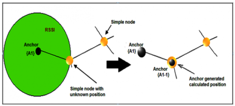
Our contribution is based on the calculation of the RSSI (Received Signal Strength Indicator) to locate the neighboring node (see Figure 3) which is one hop away from an anchor, and to take advantage of this position as a new anchor node, this facilitates the iteration of the position searching of the other nodes that have not yet been located.
Figure 3. Illustration of the proposed approach
Our localisation proposal is implemented on the Contiki-OS operating system, using its Cooja Simulator. This system provides us with most of the basic elements needed to emulate a sensor network. Thus, a set of nodes are deployed in an environment with a square area of [100 m × 100 m]. We have taken in our sample 5% of sensor-anchors, whose positions (xi, yi) are known, among N unknown nodes that seek to estimate their positions using these main anchors.
4.2 Problem formulation
Our work can be summarized in the following steps:
1. Calculation of the distance error rate:
-Anchor nodes broadcast "Hello|1" messages on the network, containing location and identification information (see Table 1). This first step consists of identifying the direct neighboring nodes.
Table 1. Structure of a "Hello|1" anchor package
|
IdA |
xi |
yi |
Hop-Count |
-All nodes contain a small memory where information from the different nodes of the networks is stored (see Table 2).
Table 2. Structure of a node's buffer
|
IdA |
x i |
yi |
CISOU |
drU |
drT |
Hop-Count |
-IdA: identifier of the anchor node.
-(xi, yi): Geographical coordinates of the nodes.
-Hop-Count: number of hops, set to 0.
-drU: Actual distance calculated by RSSIN from the anchor node to the unknown node {U?}.
-U?: Nodes with unknown location.
-drT: Total cumulative distance.
-Hop-Count: Cumulative hop count.
-Initially the Hop-Count field of each unknown node {U?} is set to zero (0).
-Each unknown node receiving a "Hello|1" message from an anchor, checks its existence in its memory. In the case where the anchor identifier does not exist, the unknown node {U?} updates its memory table, calculating the distance to the sending anchor and incrementing "Hop-count" by "1", to note that it is one hop away from the anchor, then broadcasts the new "Hello|1" packet across the network. However, if the "IdA" identifier exists on its table, a comparison of the minimum hop-count is necessary to know whether or not to modify the table.
-Anchor nodes store messages with a minimum hop-count.
-Once the convergence of the network is reached, the anchors proceed to calculate the distance error rates according to Eq. (9). A second "Hello|2" message will be generated (see Table 3), and broadcast in the network.
$\tau_{E i}=\frac{\sum_{i=1}^N\left[1-\left(\frac{D_{\text {eucl }}}{D r_{T_i}}\right) / H o p-\text { Count }_i\right]}{N}$ (9)
-Deucl: Euclidean distance
-N: Total number of anchors in the network.
Table 3. Structure of the second "Hello|2" package.
|
IdA |
Type_id |
xi, |
yi |
Hop-Count |
$\boldsymbol{\tau}_{\mathrm{Ei}}$ |
2. Calculation of the position of the nodes
-Same scenario as the previous step, only messages received with minimum Hop-Counts will be retained and/or incremented and broadcast.
-If an unknown node {U?} receives three or more messages from the anchor nodes including at least one neighbouring anchor then the unknown node calculates its coordinates according to the following rules:
●If the distance between the unknown node and the anchor is one hop then the node calculates the actual distance (drU) directly via RSSI.
●If the distance between the unknown node and the anchor is equal to more than one hop then the distance will be calculated by multiplying the total distance by the distance error rate according to Eq. (10).
$\operatorname{Dist}_{U ?}^A=d r_T \cdot\left[1-\left(\tau_{E i} \times(\right.\right.$ Hop-Count $\left.)\right]$ (10)
-Once the distance has been calculated, the unknown node estimates its geographical position and changes its type (Type-id = anchor) and in turn becomes an anchor.
- An unknown node {U?} ignores all messages sent by non-direct neighbour anchors.
3- Update of node positions:
- If a node receives a message from another node that has just been initiated as an anchor and the distance between them is one hop (Hop-Count=1), then that node recalculates its position and updates its table. Otherwise, the message is ignored.
4.3 Our "DVA-Hop" algorithm
Our "Distance Vector Adjusted-Hop" algorithm, nicknamed "DVA-Hop", takes its form from the traditional "DV-Hop" algorithm but introduces an error rate calculation as follows.
The experiment is performed on the Contiki-OS Java Simulator (see Figure 4) which is a sensor network emulator supporting a compiled program in order to verify a scenario before it is loaded into the flash memory of the real nodes as in the TI-MSP430 platform. Thus, we configured the simulator to a number of parameters, (see Table 4).
Table 4. Simulation parameters.
|
Parameters |
Values |
|
Size of the map |
100 × 100 m |
|
Number of sensor nodes |
100 |
|
Number of anchors |
5 |
|
Communication radius (metres) |
30 |
|
Number of iterations |
10 |
Algorithm DVA-Hop;
1: Initialization of the algorithm.
2: Input N
3: For i=1 to N;
Anchors prepare the first messages « Hello|1 » with {Coordinates, « Hop-count » = 0};
The Anchors broadcast their messages;
4: End-For
5: An unknown-node {N?} receives the message « Hello|1 » and tests the « Hop-count »;
6: If « Hop-count » = minimum then
« Hop-count » = « Hop-count » +1;
Calculate the distance of the message using the « RSSI »;
Calculates the cumulative distance travelled by the message;
Update then resends the new message on the network;
Else do nothing;
7: End-if;
8: Each Anchor computes error rate « $\boldsymbol{\tau}_{\mathrm{Ei}}$ »;
9: Broadcast « Hello|2 » with « $\boldsymbol{\tau}_{\mathrm{Ei}}$» on the network;
10: If unknown node has at least one neighboring anchor then
Select the closest anchors and nodes (« Hop-count », « drT »);
Unknown node calculates its position;
This knot becomes an additional anchor;
Back to 3:
11: End if;
12: End;
Figure 4. Cooja/Contiki simulator
We used the mean square error Eq. (11) to estimate the positioning accuracy. Thus, to calculate the mean location error, we measure the distance of the link point calculated by our algorithm to its corresponding real position point.
The average location error noted:
${ }_{a v g} \operatorname{Err}^{L o c}=\frac{100}{M \times R} \sqrt{\left(x_i^{\prime}-x_i\right)^2+\left(y_i^{\prime}-y_i\right)^2}$ (11)
(xi, yi): Actual geographical position of the sensor node.
$\left(x_i^{\prime}, y_i^{\prime}\right)$ : Estimated geographical position of the node.
M: Number of unknown nodes.
R: Communication radius of the node.
5.1 Comparison of the localisation error as a function of the number of single nodes
Figure 5. Location error comparison framework (05 fixed anchors)
A first simulation, applying the two algorithms, "DV-Hop" and "DVA-Hop", was carried out to demonstrate the scaling of our experiments. In this sense, we calculated the localisation error in meters for a number of 100(nodes?), on a stable number of anchors equal to 5.
The results are shown in the graph in Figure 5, highlighting a reduction in error as the number of single nodes increases. This is explained on one hand by the increase in the number of hops between neighboring nodes and consequently an accumulation of error, and on the other hand by the use of a small monitoring area.
We also notice that the accuracy of our "DVA-Hop" algorithm decreases if the density of the node distribution is low or non-uniform. Thus, the positioning gap of both algorithms decreases as the number of nodes increases.
As a result, it is noted that the more nodes in a surface to be monitored, the more the localisation error is minimized. Our "DVA-Hop" algorithm shows a clear improvement in error rate compared to the traditional "DV-Hop" algorithm.
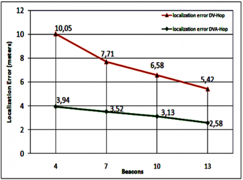
5.2 Comparison of the error as a function of the number of anchors
This simulation consists of calculating the location deviation of 100 nodes with 4, 7, 10 and 13 anchors respectively. In this experiment, we maintained the geographical positions of the beacon nodes, with a radio communication radius of 30 meters.
Figure 6. Location errors as a function of the number of anchors
We observe in Figure 6 that the more the number of beacon nodes is large, the smaller the positioning intervals of both algorithms become, underlining the satisfactory result of our algorithm. This is due to the fact that the information from the unknown node transits through several hops to reach the nearest anchor, amplifying the average error of the hop. Finally, we can conclude that:
1. The distance difference between our "DVA-Hop" and "DV-Hop" algorithm increases with the number of jumps.
2. The reduction in deviation, between our "DVA-Hop" and "DV-Hop" algorithm, is the consequence of the increase in the number of anchors.
5.3 Energy assessment of the proposed algorithm
In order to determine the efficiency of our algorithm, a second aspect is the evaluation of the energy consumption of unknown anchors and nodes (see Figure 7).
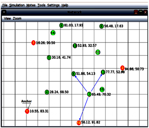
The number of nodes is reduced, in order to speed up the response time of the simulation. The default radio model is the "Unit Disk Graph Medium" or "UDGM Distance Loss". The simulation parameters are shown in Table 5.
Figure 7. Simulation scenario: Node positions on Cooja/Contiki
Table 5. Energy simulation parameters
|
Parameters |
Values |
|
Radio model |
UDGM |
|
Type of nodes |
Skymote |
|
Unknown nodes |
11 |
|
Number of anchors |
04 |
|
Transmission area |
30 m |
|
Interference zone |
100 m |
|
Transmission ratio |
100 % |
|
Reception ratio |
100 % |
|
Deployment |
Random |
|
Simulation time |
20 min |
|
Network dimension |
100m x100m |
The total energy consumed by a sensor node is given by the following Eq. (12):
Energynoeud=EnergyCPU+EnergyLPM+EnergyTX+EnergyRx (12)
Knowing that the four modules of a node that consume energy are:
-CPU: Number of clock ticks of the processor in active state, without radio modules.
-LPM: Number of clock ticks in standby state.
-TX: Number of clock ticks in transmission state.
-RX: Number of clock ticks in reception state.
Thus, we can calculate the energy consumption of each module in milliwatts using the following Eq. (13) using the parameters of the node type, in our case "Skymote":
Energymodule=Emodule*C*V/(Rtimer_Second)*Runtime (13)
-Emodule: This is the difference in the Ticks number of the "CPU module", for example, between two-time intervals.
-C (Current): Current intensity $(\mathrm{CPU} \simeq 330 \mu \mathrm{A}, \mathrm{LPM} \simeq 1.1 \mu \mathrm{A}, \mathrm{Tx} \simeq 17.4 \mathrm{~mA}, \mathrm{Rx} \simeq 18.8 \mathrm{~mA}$,
-V: Voltage $(\simeq 3 \mathrm{Volt})$
-Rtimer_Second: Low frequency crystal frequency $(\simeq 32768 \mathrm{Ticks} / \mathrm{s})$.
-Runtime: Powertrace runtime $(\simeq 5$ seconds $)$.
-One Ticks system is equivalent to 1 millisecond.
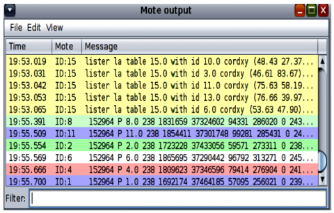
After starting the simulation, Figure 8 shows some positional information, and the information needed for the energy calculation.
Calculation of the average consumption of the four anchors:
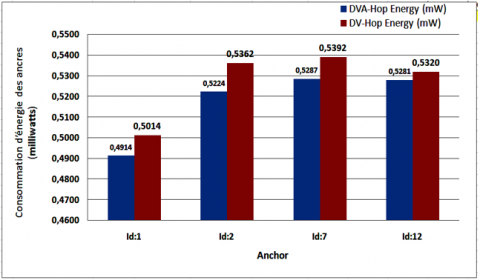
The energy consumed by the anchors, after extracting the information from the Ticks, and applying Eq. (13) to calculate the energy consumed by each module. The total energy of each node, "anchor", is calculated using Eq. (12), the result obtained is shown in Figure 9 below.
Figure 8. Energy simulation scenario on Cooja/Contiki
Figure 9. Energy consumed by each "anchor" node
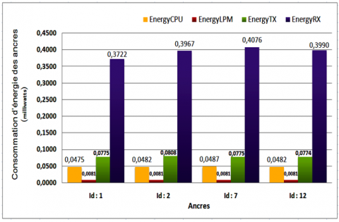
Figure 10. Energy consumed by each module of the "anchor" "DVA-Hop" nodes
The experiment reveals that the anchor with id:7 consumed slightly more energy than the others, given that the concentration of most of the nodes are in its proximity. This slight increase in energy consumed by anchor 07 during 20 minutes of simulation, although negligible, could be justified by the amount of energy consumed by the radio module either in data reception (Rx), or in transmission (Tx), and more or less in processing energy. But, as for the Idle Listening energy, it remains almost negligible. Figure 9 shows that our approach is still distinguished by the reduced energy consumption.
Figure 10 shows the node modules responsible for this increase in energy consumption in our DVA-Hop algorithm.
Another geometrical interpretation can be elucidated on this energetic elevation of the anchor id:7 and the anchor id:2. It can be seen that these anchors have three nodes in the vicinity, which leads to a dense communication on the network, and therefore a higher listening energy (see Figure 10).
Average energy consumption of single nodes:
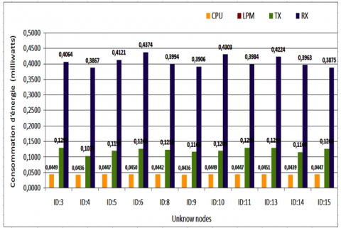
A study on the energy consumption of single nodes was carried out to estimate the lifetime of our network. Figure 11 shows that node id:6 consumed a rather high amount of energy. We will explain this increase by its central position, and acts as a transit node for the rest of the network. In addition, Idle Listening with the absence of sleep mode during periods of inactivity of the radio module plays a very important role.
Figure 11. Energy consumed by each module of the unknown nodes
Note: We notice that the radio reception module consumes more energy than the others. Therefore, in order to save energy, it is better to activate the "Duty cycle", i.e., a sleep state (alternating between active and sleep mode).
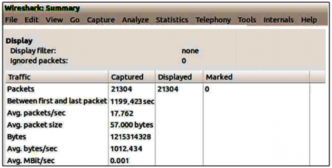
Figure 12. DVA-Hop Latency: Wireshark
Calculation of the average latency with Wireshark:
The average latency of a network is the time taken for a packet to travel from a sending node to a receiving node.
The simulation time is set to 20 minutes. During this time, a fairly high communication rate of around 21301 packets was noted, (see Figure 12), which has a direct influence on the energy consumption of the nodes (see Table 6).
Table 6. Latency derived by Wireshark.
|
Parameters |
DVA-Hop values |
DV-Hop values |
|
Total nodes |
15 |
15 |
|
Simulation time |
$\simeq$20 min |
$\simeq$20 min |
|
Number of distributed packages |
21301 |
17836 |
|
Size of a packet (Byte) |
57 |
57 |
|
Average Packets/s |
17.762 |
14.870 |
|
Average Latency (s) |
0.0569 s |
0.0672s |
We note that the average packet size, although fixed, is 57 bytes in our simulation, and the latency of our algorithm is better than that of the traditional DV-hop.
Wireless sensor networks have been the subject of much research, both in industry and academia. This is due to the unprecedented breadth of possibilities offered by this technique. However, wireless sensor networks also face significant challenges in locating randomly distributed nodes in hostile or inaccessible locations.
In this paper, we have presented an improvement of the DV-Hop algorithm by a mixed approach to locate unknown nodes. The method relies on two mechanisms for position calculation: the received signal strength "RSSI", and the Hop averaging principle "DV-Hop", in order to increase the geographical accuracy of unknown nodes. This is a stimulating perspective because the RSSI signal strength is delivered with the data packets when they are received, which does not incur any additional cost in terms of new hardware components or power consumption. In addition, our algorithm gradually discovers unknown nodes surrounding the anchors, and substitutes them into beacons to complete the localisation process.
A comparison framework explains the encouraging result and the clearly observed performance of our approach, not only in the improvement of the average Hop but also in the advantage of sustaining the network by saving energy on one hand and optimizing latency on the otherhand.
[1] Benaissa, B.E., Lahfa, F., Naima, K., Lorenzini, G., Inc, M., Menni, Y. (2021). Detection and cooperative communications for deployment sensor networks. Traitement du Signal, 38(3): 555-564. https://doi.org/10.18280/ts.380303
[2] Rabhi, S., Semcheddine, F. (2019). Localization in wireless sensor networks using DV-hop algorithm and fruit fly meta-heuristic. Advances in Modelling and Analysis B, 62(1): 18-23. https://doi.org/10.18280/ama_b.620103
[3] Yuan, R.L. (2020). Positioning of wireless sensor network under emergency communication environment. Instrumentation Mesure Métrologie, 19(4): 273-279. https://doi.org/10.18280/i2m.190404
[4] Zhao, W., Shao, F., Ye, S., Zheng, W. (2018). LSRR-LA: An anisotropy-tolerant localization algorithm based on least square regularized regression for multi-hop wireless sensor networks. Sensors, 18(11): 3974. https://doi.org/10.3390/s18113974
[5] Miao, Y.S., Wu, H.R., Zhu, H.J., Song, Y.L. (2018). Localization accuracy of farmland wireless sensor network localization algorithm based on received signal strength indicator, Ingénierie des Systèmes d’Information, 23(5): 69-80. https://doi.org/10.3166/ISI.23.5.69-80
[6] Rabhi, S., Ouahab, A., Baddou, S., Chetouah, K. (2021). An improved algorithm based on chicken swarm optimization for localization in wireless sensor networks. Advances in Modelling and Analysis B, 64(1-4): 34-39. https://doi.org/10.18280/ama_b.641-405
[7] Niculescu, D., Nath, B. (2003). DV based positioning in ad hoc networks. Telecommunication Systems, 22(1): 267-280. https://doi.org/10.1023/A:1023403323460
[8] Lu, J.Y. (2019). A new distance vector-hop localization algorithm based on half-measure weighted centroid. Mobile Information Systems, 2019: 9892512. https://doi.org/10.1155/2019/9892512
[9] Prashar, D., Jyoti, K. (2019). Distance error correction based hop localization algorithm for wireless sensor network. Wireless Personal Communications, 106: 1465-1488. https://doi.org/10.1007/s11277-019-06225-0
[10] Spilker Jr, J.J., Axelrad, P., Parkinson, B.W., Enge, P. (1996). Global Positioning System: Theory and Applications, volume I. American Institute of Aeronautics and Astronautics.
[11] Hu, Y., Shan, Z., Yu, H. (2012). Research on improved DV-HOP localization algorithm based on the ratio of distances. In Internet of Things, pp. 118-125. https://doi.org/10.1007/978-3-642-32427-7_17
[12] Hu, Y., Li, X. (2013). An improvement of DV-Hop localization algorithm for wireless sensor networks. Telecommunication Systems, 53(1): 13-18. https://doi.org/10.1007/s11235-013-9671-8
[13] Liu, F., Feng, G. Z. (2015). Research on improved dv-hop localization algorithm based on RSSI and feedback mechanism. In China Conference on Wireless Sensor Networks, Xi'an, China, pp. 144-154. https://doi.org/10.1007/978-3-662-46981-1_14
[14] Yuan, R.L. (2020). Positioning of wireless sensor network under emergency communication environment. Instrumentation Mesure Métrologie, 19(4): 273-279. https://doi.org/10.18280/i2m.190404
[15] Kanwar, V., Kumar, A. (2021). DV-Hop localization methods for displaced sensor nodes in wireless sensor network using PSO. Wireless Networks, 27(1): 91-102. https://doi.org/10.1007/s11276-020-02446-5