OPEN ACCESS
The purpose of this study is to investigate homogeneous-heterogeneous reaction with second order resistance for Casson fluid in stagnation point flow and Falkner-Skan flow on the presence of induced magnetic field and non-uniform heat source. The governing partial differential equations are transformed into ordinary differential equations and solved numerically by fourth fifth order Runge-Kutta Fehlberg method (RKF45) with shooting technique. The effects of different physical parameters on velocity profile, induced magnetic profile, temperature profile and species concentration profile are presented through graphical and tabular form. The finding of this study may serve many areas including catalysis, combustion and biochemical systems. The scope of this study is to comparison two structures viz. Falkner-Skan Flow and Stagnation-Point flow.
Homogeneous-heterogeneous, Falkner-Skan flow, Casson fluid, Induced magnetic field, Second order resistance
Researchers and scientists have been still attracted towards the investigation of flow behavior in the neighborhoods of stagnation point due to its wide applications in the engineering, industrial processes and natural phenomena. Stagnation point occurs in the various flow models including two-dimensional, three-dimensional, symmetric, asymmetric, inviscid, viscous steady, unsteady, forward, reverse, normal or oblique, homogeneous, immiscible fluids, etc. The flow over the rockets, tips of submarines, oil ships and aircrafts are the application of stagnation point flow. Several exact solutions of the non-linear NS equations have been found by considering different geometries Chiam (1994). Stagnation-point flow over a stretching plate was studied by Chiam (1994). Wang (2008) presented the solution of stagnation-point flow near the shrinking sheet. He solved the partial governing equation with the help of suitable transformations. Ishak et al. (2009) discussed MHD boundary layer stagnation-point flow past a stretching sheet and presented the results through graphs and tables. Chauhan et al. (2011; 2011) analyzed heat transfer effects of MHD boundary layer flow over a stretching sheet and plate, respectively. Recently, Bayat et al. (2017) studied the case of three-dimensional Navier-Stokes equations in the presence of stagnation point flow over the rotating vertical cylinder.
The flow past a wedge has been broadly studied by several researchers due to its applications in heat exchangers, geothermal systems, aerodynamics etc. Furthermore, the flow over a wedge is important due to the fact that each and every value of the wedge angle produces a diverse pressure profile, thereby contribution insight into boundary layer behavior in number of situations. Many researchers explored, expanded features of such problems and few studied regarding boundary layer flow over a wedge. Falkner and Skan (1931) gave the exact solutions for the boundary layer flow over a wedge. After that, this type of the flow was renamed as “Falkner-Skan” flow in the memory of Fankner and Skan. Several authors such as Rajagopal et al. (1983) Lin et al. (1987), Ganapathirao et al. (2015) Kasmani et al. (2016) and Khan et al. (2017) were investigated the boundary layer phenomenon towards a wedge in the presence of pertinent parameters.
MHD is the study of motion of electrically conducting fluid in the existence of magnetic field. The mathematical models having induced magnetic field have a wide industrial application such as in liquid-metals, fiber or granular insulation, electrolytes, ionized gases and geothermal systems. The influence of a magnetic field with the induced magnetic field in the boundary layer flow were considered by some authors such as Raptis and Perdikis (1984) examined the behavior of free convection in the existence of magnetic field with different parameter. They investigated, the study of motion of electrical conduction fluid with magnetic field. Ishak et al. (2009) investigated the effects of MHD boundary layer on a moving wedge. Ali et al. (2012) presented the effects of MHD over a stretching sheet in the presence of the induced magnetic field with radiation. They observed that the viscous dissipation may cause thermal reversal near the surface which is sustained by the stretching parameter of the sheet when higher than unity and the Prandtl number as well. Ali et al. (2011), Jafar et al. (2013), Jain and Choudhary (2015), El-Dabe et al. (2015), Jain and Bohra (2016), Gireesha et al. (2016) and Srinivasacharya and Shafeeurrahman (2017) have been studied the MHD phenomenon with different geometries in the existence of various parameters.
The role of Non-Newtonian fluids in boundary layer flow, such as Casson fluid is most useful in many areas, for example petroleum drilling, polymer processing industries and many more. Casson fluid is one of the supreme fluid which presents the yield stress effects. This fluid is considered as a shear thinning liquid which has zero viscosity at an infinite rate of shear (1959). In similar words, this type of fluid’s behavior changes with shear stress. Casson boundary layer fluid flow towards a stretching sheet for the unsteady case investigated by Mukhopadhyay et al. (2013). Heat transfer effects of Casson fluid in boundary layer flow with radiative conditions were analyzed by Pramanik (2014). Raju et al. (2017) scrutinized the magnetohydrodynamics effects for Casson fluid towards a moving geometry with heat source/sink.
Many chemically reacting systems has contained homogeneous and heterogeneous reactions. These types of reaction have many applications including catalysis, combustion and biochemical systems. The interface between the homogeneous reactions in bulk of the fluid and heterogeneous reactions taking place on some catalytic surfaces is commonly very difficult, which is incorporated in the generation and consumption of reactant species at different rates both within the fluid and on the catalytic surfaces. Initially, Chaudhary and Merkin (1995) and Merkin (1996) gave a model for homogeneous-heterogeneous reactions in the boundary layer flow near the surface. In this case a simple model for homogeneous-heterogeneous reactions in stagnation-point boundary-layer flow is created in which the homogeneous (bulk) reaction is supposed to be given by isothermal cubic auto catalator kinetics and the heterogeneous (surface) reaction by first order kinetics. Abbas et al. (2015) investigated the effects of homogeneous-heterogeneous reactions over a shrinking/stretching sheet in the presence of MHD. Further, Animasaum et al. (2016) and Khan et al. (2017) also studied the homogeneous-heterogeneous reactions for various geometries.
In addition, no studied have been done before for the comparative study of Stagnation-point flow and Falkner-Skan flow of Casson boundary layer fluid flow with the effects of homogeneous-heterogeneous reaction in the presence of the induced magnetic field, first and second order resistance due to inertia force and non-uniform heat source. Using the applicable transformation, the boundary layer equations are reduced into non-linear ordinary differential equations and results are shown through the graphical representations and tabular form.
We consider a steady, laminar, two-dimensional boundary layer Casson fluid flow and hydromagnetic coupled heat transfer through porous media, over a moving plate and a moving wedge in the presence of variable induced magnetic field and non-uniform heat source. Effect of second order resistance and homogeneous-heterogeneous reactions has also been discussed (figure 1). We assumed that the velocity and free stream velocity of the moving wedge are uw(x)=Uwxm and ue(x)=U∞xm, respectively, where $\lambda = \frac { 2 m } { m + 1 } = \frac { \Omega } { \pi }$ is known as Hartree pressure gradient parameter, where $\Omega$ is the total angle of moving wedge and m is a constant. In this study, we have studied both Stagnation-Point flow and Falkner-Skan flow that means flow over a plat when m=1 and over a wedge when m=0.5.
(a) (b)
Figure 1. (a) Stagnation-Point flow (m=1) and (b) Falkner-Skan Flow (m=0.5)
Rheological model that defines Casson fluid is
$\tau _ { i j } = \left\{ \begin{array} { l } { 2 \left( \mu _ { B } + p _ { y } / \sqrt { 2 \pi } \right) e _ { i j } , \pi > \pi _ { c } } \\ { 2 \left( \mu _ { B } + p _ { y } / \sqrt { 2 \pi _ { c } } \right) e _ { i j } , \pi < \pi _ { c } } \end{array} \right.$ (1)
where, τijis the component of the stress tensor, pyis the yield stress of the fluid, π is the product of the component of the deformation rate with itself, πc is a critical value of this product established on the non-Newtonian model and µB is the plastic dynamic velocity of the non-Newtonian fluid.
We have taken model for the interaction between homogenous and a heterogeneous reaction for both wedge and plate, including two chemical species A and B in a boundary layer flow [follows Chaudhary and Merkin (1995) and Merkin (1995) given as:
The homogeneous reaction for cubic autocatalysis is given as:
$A + 2 B \rightarrow 3 B ,$ rate $= k _ { c } a b ^ { 2 }$ (2)
First order isothermal reaction on the catalyst surface is given as:
$A \rightarrow B ,$ rate $= k _ { s } a$
Where a and b are the concentration of the chemical species A and B, kc and ks are the rate constants. These equations confirm that both in the external flow as well as at the outer edge of the boundary layer, the reaction rate is zero. Also, it is assumed that the reaction process is isothermal. Here we take the Cartesian coordinators x-axis along with the surface of the wedge and the plate and y-axis is normal to it, correspondingly. We assume that (u, v) and (H1, H2) are the velocity and magnetic components along (x, y) directions, respectively.
According to above boundary layer assumptions, governing equations are [follows (Jain and Choudhary, 2015; Raptis and Perdikis, 1984)] given as:
$\frac { \partial u } { \partial x } + \frac { \partial v } { \partial y } = 0$ (3)
$\frac { \partial H _ { 1 } } { \partial x } + \frac { \partial H _ { 2 } } { \partial y } = 0$ (4)
$u \frac { \partial u } { \partial x } + v \frac { \partial u } { \partial y } = u _ { e } \frac { d u _ { e } } { d x } + v \left( 1 + \frac { 1 } { \beta } \right) \frac { \partial ^ { 2 } u } { \partial y ^ { 2 } } + \frac { \mu _ { 0 } } { 4 \pi \rho } \left( H _ { 1 } \frac { \partial H _ { 1 } } { \partial x } + H _ { 2 } \frac { \partial H _ { 1 } } { \partial y } \right) - \frac { \mu _ { 0 } } { 4 \pi \rho } H _ { e } \frac { d H _ { e } } { d x }$$- \frac { v } { k } \left( u - u _ { e } \right) - F \left( u ^ { 2 } - u _ { e } ^ { 2 } \right)$ (5)
$u \frac { \partial H _ { 1 } } { \partial x } + v \frac { \partial H _ { 1 } } { \partial y } - H _ { 1 } \frac { \partial u } { \partial x } - H _ { 2 } \frac { \partial u } { \partial y } = \mu _ { e } \frac { \partial ^ { 2 } H _ { 1 } } { \partial y ^ { 2 } }$ (6)
$u \frac { \partial T } { \partial x } + v \frac { \partial T } { \partial y } = \alpha \frac { \partial ^ { 2 } T } { \partial y ^ { 2 } } + \frac { q ^ { \prime \prime \prime } } { \rho C _ { p } }$ (7)
$u \frac { \partial a } { \partial x } + v \frac { \partial a } { \partial y } = D _ { A } \frac { \partial ^ { 2 } a } { \partial y ^ { 2 } } - k _ { c } a b ^ { 2 }$ (8)
$u \frac { \partial b } { \partial x } + v \frac { \partial b } { \partial y } = D _ { B } \frac { \partial ^ { 2 } b } { \partial y ^ { 2 } } + k _ { c } a b ^ { 2 }$ (9)
Subject to the boundary conditions:
$u = u _ { w } ( x ) = U _ { w } x ^ { m } , v = 0 , H _ { 1 } = H _ { 2 } = 0 , T = T _ { w } , D _ { A } \frac { \partial a } { \partial y } = k _ { s } a , D _ { B } \frac { \partial b } { \partial y } = - k _ { s } a$ at y = 0
$u = u _ { e } ( x ) = U _ { \infty } x ^ { m } , H _ { 1 } = H _ { e } ( x ) = H _ { 0 } x ^ { m } , T = T _ { \infty } , a \rightarrow a _ { 0 } , b \rightarrow 0 { \text {as } } y \rightarrow \infty$ (10)
The proposed problem shows two-different geometries based on the following assumptions:
(i) m = 1 (Stagnation point flow)
(ii) m = 0.5 (Falkner-Skan flow)
where $\beta = \mu _ { B } \sqrt { 2 \pi _ { c } / \rho _ { y } }$ is the Casson fluid parameter, T is the temperature, Tw is the temperature at the wall, T∞ is the ambient temperature, ue(x) and He(x) are the x-axis velocity and magnetic field at the edge of the boundary layer, correspondingly, k is the permeability, F is the empirical constant of the second order resistance term due to the inertia effect, H is the induced magnetic field vector, $\mu _ { 0 }$ is the magnetic permeability, ρ is the fluid density, $\mu _ { e } = 1 / 4 \pi \sigma$ is the magnetic diffusivity, $\alpha = \kappa / \rho C _ { p }$ is the thermal diffusivity, $\kappa$ is the thermal conductivity, $C_p$is the specific heat at constant pressure. DA and DB are respective diffusion coefficients.
The space and temperature dependent non-uniform heat source/sink is as follows:
$q ^ { \prime \prime \prime } = \frac { k u _ { e } ( x ) } { x v } \left[ A ^ { * } \left( T _ { w } - T _ { \infty } \right) f ^ { \prime } ( \eta ) + B ^ { * } \left( T - T _ { \infty } \right) \right]$ (11)
Where, v is the kinematic fluid viscosity, A* and B* are the space and temperature dependent heat source/sink parameter.
To solve the system of equations (3)-(9), are converted into dimensionless form by introducing the following similarity transformation:
$\eta = \sqrt { \frac { ( m + 1 ) u _ { e } ( x ) } { 2 v x } } y \quad \psi = \sqrt { \frac { 2 \nu x u _ { e } ( x ) } { ( m + 1 ) } } f ( \eta ) \quad \phi = H _ { 0 } \sqrt { \frac { 2 v x ^ { m + 1 } } { ( m + 1 ) U _ { \infty } } } s ( \eta )$ $a = a _ { 0 } g ( \eta ) \quad , \quad b = a _ { 0 } h ( \eta ) , \quad \theta = \frac { T - T _ { \infty } } { T _ { w } - T _ { \infty } }$ (12)
Where $f ( \eta )$ is the stream function, $s ( \eta )$ is the induced magnetic field, $\theta ( \eta )$is the temperature and $g ( \eta )$$h( \eta )$ are the concentrations.
The equation of continuity and equation of induced magnetic field is satisfied automatically on introducing following functions:
$u = \frac { \partial \psi } { \partial y } , v = - \frac { \partial \psi } { \partial x } \quad H _ { 1 } = \frac { \partial \phi } { \partial y } , H _ { 2 } = - \frac { \partial \phi } { \partial x }$ (13)
Using equations (12) - (13), equations (5)-(9) reduces in following equations:
$\left( 1 + \frac { 1 } { \beta } \right) f ^ { \prime \prime \prime } + f f ^ { \prime \prime } + \lambda \left( 1 - f ^ { \prime 2 } \right) + M ^ { 2 } \left( \lambda s ^ { \prime 2 } - s s ^ { \prime \prime } \right) - M ^ { 2 } \lambda$ $- K \left( f ^ { \prime } - 1 \right) - \Delta \left( f ^ { \prime 2 } - 1 \right) = 0$ (14)
$\lambda ^ { * } s ^ { \prime \prime \prime } + f s ^ { \prime \prime } - f ^ { \prime \prime } s = 0$ (15)
$\theta ^ { \prime \prime } + \operatorname { Pr } f \theta ^ { \prime } + ( 2 - \lambda ) \left( A ^ { * } f ^ { \prime } - B ^ { * } \theta \right) = 0$ (16)
$\frac { 1 } { S c } g ^ { \prime \prime } + f g ^ { \prime } - K ^ { * } g h ^ { 2 } = 0$ (17)
$\frac { \delta ^ { * } } { S c } h ^ { \prime \prime } + f h ^ { \prime } + K ^ { * } g h ^ { 2 } = 0$ (18)
Subject to the following boundary conditions
$f ( 0 ) = 0 , f ^ { \prime } ( 0 ) = \gamma , s ( 0 ) = 0 , s ^ { \prime } ( 0 ) = 0 , \theta ( 0 ) = 1 , g ( 0 ) = g ^ { \prime } ( 0 ) / K _ { s }$ $h ^ { \prime } ( 0 ) = - K _ { s } g ( 0 ) / \delta ^ { * }$
$f ^ { \prime } ( \infty ) \rightarrow 1 , s ^ { \prime } ( \infty ) \rightarrow 1 , \theta ( \infty ) \rightarrow 0 , g ( \infty ) \rightarrow 0 , h ( \infty ) \rightarrow 0$ (19)
where
$\lambda = \frac { 2 m } { m + 1 } \quad M ^ { 2 } = \frac { \mu H _ { 0 } ^ { 2 } } { 4 \pi \rho U _ { \infty } ^ { 2 } } \quad K = \frac { 2 v x } { k ( m + 1 ) U _ { \infty } x ^ { m } } \quad \Delta = F x \frac { 2 } { m + 1 } \quad \lambda ^ { * } = \frac { 1 } { 4 \pi \sigma v }$ $S c = \frac { v } { D _ { A } } \quad K ^ { * } = \frac { 2 k _ { c } a _ { 0 } ^ { 2 } } { ( m + 1 ) U _ { \infty } x ^ { m - 1 } } \quad \delta ^ { * } = \frac { D _ { B } } { D _ { A } } \quad \gamma = \frac { U _ { w } } { U _ { \infty } } \quad K _ { s } = \frac { k _ { s } R _ { e } ^ { - 1 / 2 } } { D _ { A } } R _ { e } = \frac { u _ { e } ( x ) x } { v }$
Hartree pressure gradient, the magnetic parameter, inertia coefficient parameter, permeability parameter, reciprocal of magnetic Prandtl number, Schmidt number, measure of the strength of the homogeneous reaction, the ratio of diffusion coefficients, moving wedge parameter, measure of the strength of the heterogeneous reaction and local Reynolds number, respectively.
In many industrial process, It is preferred that the size of diffusion coefficients of chemical species A and B are comparable, in this view, assumed that the diffusion coefficients DA and DB are equal, Following (Raptis and Perdikis, 1984), we take δ=1, and obtain a relation given as:
$g ( \eta ) + h ( \eta ) = 1$ (20)
Using equation (20), equations (17)-(18) reduces into in single equation given as
$\frac { 1 } { S c } g ^ { \prime \prime } + f g ^ { \prime } - K ^ { * } \left( 1 - g ^ { 2 } \right) = 0$ (21)
subject to the boundary conditions
$g ^ { \prime } ( 0 ) = K _ { s } g ( 0 ) , g ( \infty ) \rightarrow 1 { \text {as } } \eta \rightarrow \infty$ (22)
The skin friction coefficient Cfx and local Nusselt number Nux (follows (Chiam, 1994)) given as
$C f _ { x } = \frac { \tau _ { w } } { \rho u _ { e } ^ { 2 } } , \quad N u _ { x } = \frac { x q _ { w } } { k \left( T _ { w } - T _ { \infty } \right) }$ (23)
Where, $\tau _ { w } $ and qw are the wall skin friction, wall heat flux and wall mass flux, respectively, denoted by
$\tau _ { w } = \mu _ { B } \left( 1 + \frac { 1 } { \beta } \right) \left[ \frac { \partial u } { \partial y } \right] _ { y = 0 } , q _ { w } = - \left( \frac { \partial T } { \partial y } \right) _ { y = 0 }$ (24)
Using equation (12) and (24), equation (23) reduces to
$\left( R _ { e } \right) ^ { 1 / 2 } C f _ { x } \sqrt { \frac { 2 } { m + 1 } } = \left( 1 + \frac { 1 } { \beta } \right) f ^ { \prime \prime } ( 0 ) , \left( R _ { e } \right) ^ { - 1 / 2 } N u _ { x } \sqrt { \frac { 2 } { m + 1 } } = - \theta ^ { \prime } ( 0 )$
where, Re is the local Reynolds number.
Numerical Methods:
Governing equations (14) - (16) and (21) under the corresponding boundary conditions Eqs. (19) and (24) are solved numerically fourth fifth Runge-Kutta Fehlberg method (RKF-45) with shooting technique. Using similarity transformations boundary value problems transformed into initial value problems, this procedure is used to convert higher order nonlinear differential equations into first order ordinary differential equations. The transformed equations are given as:
$f = f _ { 1 } , f ^ { \prime } = f _ { 2 } , f ^ { \prime \prime } = f _ { 3 } , f ^ { \prime \prime \prime } = f _ { 3 } ^ { \prime }$ (25)
$s = f _ { 4 } , s ^ { \prime } = f _ { 5 } , s ^ { \prime \prime } = f _ { 6 } , s ^ { \prime \prime \prime } = f _ { 6 } ^ { \prime }$ (26)
$\theta = f _ { 7 } , \theta ^ { \prime } = f _ { 8 } , \theta ^ { \prime \prime } = f _ { 8 } ^ { \prime }$ (27)
$g = f _ { 9 } , g ^ { \prime } = f _ { 10 } , g ^ { \prime \prime } = f _ { 10 }^{\prime}$ (28)
Using equation (25)-(28), equation (14)-(16) and (21) transformed into first order ordinary differential equations given as:
$f _ { 3 } ^ { \prime } = \left( \frac { 1 } { 1 + 1 / \beta } \right) \left[ \begin{array} { l } { \Delta \left( f _ { 2 } ^ { 2 } - 1 \right) + K \left( f _ { 2 } - 1 \right) - f _ { 1 } f _ { 3 } - \lambda \left( 1 - f _ { 2 } ^ { 2 } \right) - } \\ { M ^ { 2 } \left\{ \lambda \left( f _ { 5 } ^ { 2 } - 1 \right) - f _ { 1 } f _ { 6 } \right\} - f _ { 4 } f _ { 6 } } \end{array} \right]$ (29)
$f _ { 6 } ^ { \prime } = \frac { 1 } { \lambda ^ { * } } \left( f _ { 3 } f _ { 4 } - f _ { 1 } f _ { 6 } \right)$ (30)
$f _ { 8 } ^ { \prime } = - \operatorname { Pr } f _ { 1 } f _ { 8 } - ( 2 - \lambda ) \left( A ^ { * } f _ { 2 } + B ^ { * } f _ { 7 } \right)$ (31)
$f _ { 10 } ^ { \prime } = S c \left[ K ^ { * } f _ { 9 } \left( 1 - f _ { 9 } \right) ^ { 2 } - f _ { 1 } f _ { 10 } \right]$ (32)
Subject to the boundary conditions
$f _ { 1 } ( 0 ) = 0 , f _ { 2 } ( 0 ) = \gamma , f _ { 3 } ( 0 ) = r _ { 1 } , f _ { 4 } ( 0 ) = 0 , f _ { 5 } ( 0 ) = 0 , f _ { 6 } ( 0 ) = r _ { 2 }$
$f _ { 7 } ( 0 ) = 1 , \quad f _ { 8 } ( 0 ) = r _ { 3 } , f _ { 9 } ( 0 ) = f _ { 10 } ( 0 ) / K _ { s } , f _ { 10 } ( 0 ) = r _ { 4 }$ (33)
Where r1,r2,r3 and r4 are the initial guesses for $f ^ { \prime \prime } ( 0 ) , s ^ { \prime \prime } ( 0 ) , \theta ^ { \prime } ( 0 )$ and $g ^ { \prime } ( 0 )$, respectively. These values are guessed using shooting method. The Runge-Kutta-Fehlberg (RKF-45) method is a well-accepted method to obtain the solutions of initial value problems. For present computational procedure we have chosen $\eta _ { \infty }$ as $\eta _ { 8 } ( 0 \leq \eta \leq 8 )$, the step size$\Delta _ { \eta } = 0.001$, the technique is repeated till we obtained the convergence of order 10-6.
The algorithm of RKF-45 method is written as
$y _ { m + 1 } = y _ { m } + h \left( \frac { 25 } { 216 } k _ { 0 } + \frac { 1408 } { 2565 } k _ { 2 } + \frac { 2197 } { 4104 } k _ { 3 } - \frac { 1 } { 5 } k _ { 4 } \right)$ (34)
$y _ { m + 1 } = y _ { m } + h \left( \frac { 16 } { 135 } k _ { 0 } + \frac { 6656 } { 12825 } k _ { 2 } + \frac { 28561 } { 56430 } k _ { 3 } - \frac { 9 } { 50 } k _ { 4 } + \frac { 2 } { 25 } k _ { 5 } \right)$ (35)
Equations (34) and (35) are fourth and fifth order Runge-Kutta scheme respectively.\
$k _ { 0 } = f \left( x _ { m } , y _ { m } \right)$
$k _ { 1 } = f \left( x _ { m } + \frac { h } { 4 } , y _ { m } + \frac { h k _ { 0 } } { 4 } \right)$
$k _ { 2 } = f \left( x _ { m } + \frac { 3 } { 8 } h , y _ { m } + \left( \frac { 3 } { 32 } k _ { 0 } + \frac { 9 } { 32 } k _ { 1 } \right) h \right)$
$k _ { 3 } = f \left( x _ { m } + \frac { 12 } { 13 } h , y _ { m } + \left( \frac { 1932 } { 2197 } k _ { 0 } - \frac { 7200 } { 2197 } k _ { 1 } + \frac { 7296 } { 2197 } k _ { 2 } \right) h \right)$
$k _ { 4 } = f \left( x _ { m } + h , y _ { m } + \left( \frac { 439 } { 216 } k _ { 0 } - 8 k _ { 1 } + \frac { 3680 } { 513 } k _ { 2 } - \frac { 845 } { 4104 } k _ { 3 } \right) h \right)$
$k _ { 5 } = f \left( x _ { m } + \frac { h } { 2 } , y _ { m } + \left( - \frac { 8 } { 27 } k _ { 0 } + 2 k _ { 1 } - \frac { 3544 } { 2565 } k _ { 2 } + \frac { 1859 } { 4104 } k _ { 3 } - \frac { 11 } { 40 } k _ { 4 } \right) h \right)$
We have studied the combined effects of homogeneous-heterogeneous reaction in the presence of the induced magnetic field and non-linear heat source for Casson fluid boundary layer flow over a wedge (Falkner-Skan flow) and plate (Stagnation-Point flow). The effects of various parameters such as Casson fluid parameter β, magnetic field parameter M2, reciprocal magnetic Prandtl number λ*, permeability parameter K, moving wedge/plate parameter γ, inertia coefficient parameter Δ, heat source parameter, homogeneous reaction strength parameter K*, heterogeneous reaction parameter Ks and Schmidt number Sc are presented through graphs and tables for velocity profile, induced magnetic profile, temperature profile and concentration profile.
Table 1 shows the results obtained by obtained by Rajagopal et al. (1983), Ishak et al. (2009), K. Jafar (2013), El-Dabe et al. (2009) and in present investigation.
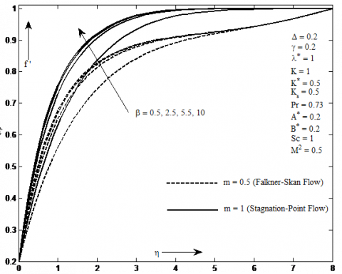
Figures (2-7) show the effects of velocity profile for various parameters. The effects of the Casson fluid parameter on velocity profile are presented in figure 2. Physically, Casson fluid parameter reduces the plasticity of the fluid. It is observed that non-Newtonian Casson fluid parameter produce resistance in the fluid flow, hence, boundary layer thickness decreases as we increase the Casson fluid parameter. The trends of stagnation-point flow is higher than the Falkner-Skan flow due to the pressure gradient.
Figure 2. Influence of casson fluid parameter on velocity profile
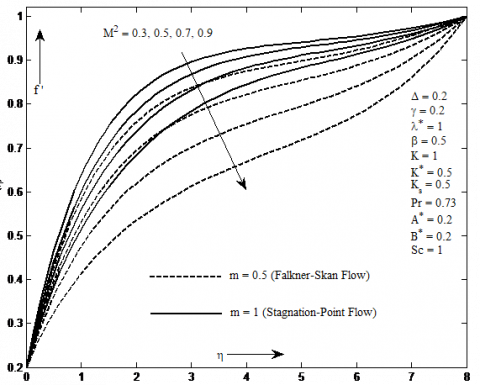
Figure 3. Influence of magnetic field parameter on Velocity profile
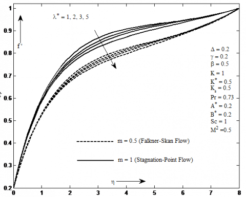
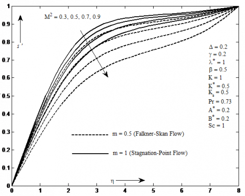
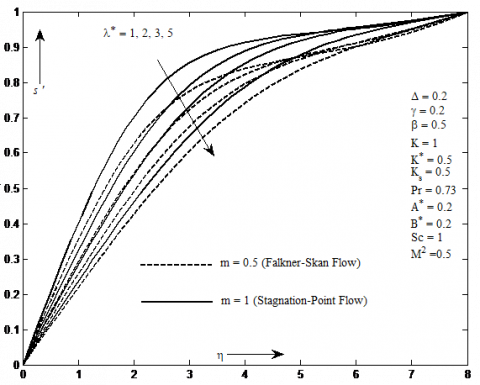
Figure 3 depicts the variation of magnetic field parameter on velocity profile. Lorentz force reduces fluid flow near the boundary layer, therefore velocity profile decreases. Similar effects have been arisen for reciprocal magnetic Prandtl number on velocity profile in figure 4. Falknar-Skan flow is decreasing more quickly than stagnation-point flow for both parameters.
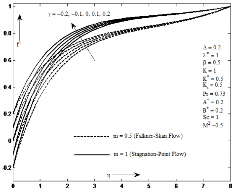
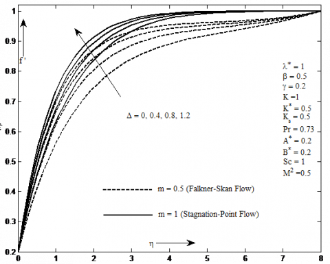
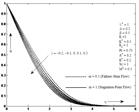
Figure 5 describes the effects of moving wedge/plate parameter on velocity profile. Increasing value of moving wedge/plate parameter leads to increase the fluid velocity, while decreases the thickness of velocity boundary layer. When moving wedge/plate parameter increases, the fluid is squeezing closer and closer to the wall, in stagnation-point flow the fluid flow is close to the wall compared to Falkner-Skan flow.
Figure 4. Influence of magnetic Prandtl number on Velocity profile
Figure 5. Influence of moving wedge/plate parameter on velocity profile
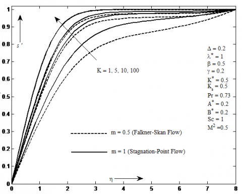
Figures 6-7 display the effects of permeability parameter and inertia coefficient parameter on velocity profile. Velocity profile is the increasing function of permeability parameter K for both types of flows, but reduces the thickness of boundary layer flow, due to the drag, which is drawn back the velocity thickness.
Figure 6. Influence of permeability parameter on velocity profile
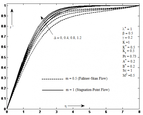
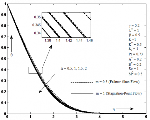
Figure 7. Influence of inertia coefficient parameter on velocity profile
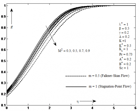
From figure 7, we conclude that the inertia coefficient parameter has the same effects as permeability parameter on velocity profile. The velocity profile is higher for stagnation-point flow compare to the Falkner-Skan flow. Figures 8-13 illustrate the effects of induced magnetic field profile for both fluid flows. Figure 8 depicts that the induced magnetic profile is the increasing function of Casson fluid parameter, it is more for stagnation point flow than Falkner-Skan flow. Figure 9 displays that as we increase magnetic field parameter, induced magnetic profile reduces. This is because the direction of the magnetic field parameter and induced magnetic profile are same.
Figure 8. Influence of casson fluid parameter on induced magnetic profile
Figure 9. Influence of magnetic field parameter on induced magnetic profile
Figure 10. Influence of magnetic Prandtl number on induced magnetic profile
Figure 11. Influence of moving wedge/plate parameter on induced magnetic profile
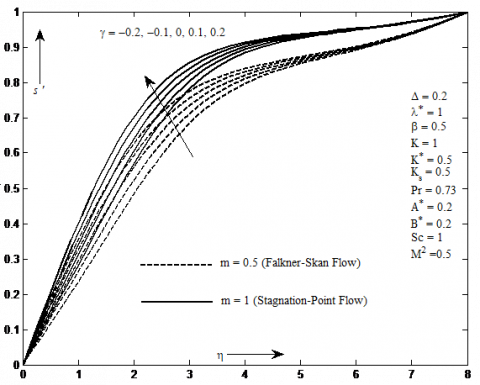
Figure 10 shows the effects of reciprocal magnetic Prandtl number for induced magnetic profile. Induced magnetic profile is decreasing as we increase reciprocal magnetic Prandtl number. From figure 11, it can be seen that induced magnetic field increases with moving wedge/plate parameter. Figures 12-13 show that induced magnetic profile is the increasing function of permeability parameter and inertia coefficient parameter. In both figures the trends of stagnation-point flow is higher than Falkner-Skan flow.
Figure 12. Influence of permeability parameter on induced magnetic profile
Figure 13. Influence of inertia coefficient parameter on induced magnetic profile
Figure 14. Influence of Casson fluid parameter on temperature profile
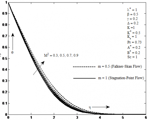
Figure 15. Influence of magnetic field parameter on temperature profile
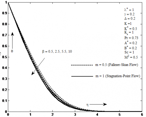
It can be observed from figure 14 that, when the value of the Casson fluid parameter is large, the fluid start to behave like Newtonian fluid, due to this reason the temperature profile is decreasing with Casson fluid parameter. If we compare stagnation-point flow and Falkner-Skan flow, we observed that temperature profile is lower for stagnation point flow than Falkner-Skan flow. Figure 15 reveals the influence of magnetic field parameter on thermal boundary layer. This implies that the impact of magnetic field parameter rises the temperature of the fluid. It is due to the resistive force that appears in the fluid flow. It is noticed that the trends of Falkner-Skan flow on temperature profile is higher when we compare it with stagnation-point flow. Figures 16-18 demonstrate the effects of moving wedge/plate parameter, permeability parameter and inertia coefficient parameter on thermal boundary layer. These parameters are working to decrease the temperature of the fluid for Falkner-Skan flow and stagnation-point flow.
Figure 16. Influence of moving wedge/plate parameter on temperature profile
Figure 17. Influence of permeability parameter on temperature profile
Figure 18. Influence of inertia coefficient parameter on temperature profile
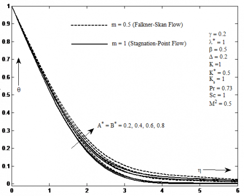
It is noticed that if permeability parameter enhances, the resistance of the porous medium is lowered, which rises the momentum development of the flow regime and ultimately reduces the temperature profile. Inertia coefficient parameter has the similar effects alike permeability parameter on temperature profile.
Heat source parameter is working to generate the heat in the fluid flow, hence it is responsible to increase the temperature profile for both cases. However, we noticed that stagnation-point flow shows the lower trends of temperature profile than the Falkner-Skan flow. These effects can be seen in figure 19.
Figure 19. Influence of heat source parameter on temperature profile
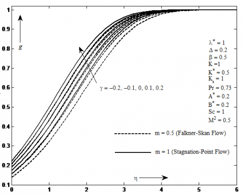
Figure 20. Influence of Casson fluid parameter on species concentration
The effects of species concentration profile for the various parameters are shown in figures 20-27. The mass transfer effects of non-Newtonian fluids in boundary layer flow is lower than Newtonian fluid. Figure 20 reveals that when fluid converting from non-Newtonian fluid to Newtonian fluid, the concentration profile increase. It is noted that concentration profile is higher for stagnation point flow. In figure 21, the concentration profile decreases with magnetic field parameter, due to the Lorentz force that works to slow down the velocity and species concentration profile.
Figure 21. Influence of magnetic field parameter on species concentration
Figure 22. Influence of moving wedge/plate parameter on species concentration
Figure 23. Influence of permeability parameter on species concentration
Figures 22-24 show the variations of moving wedge/plate parameter, permeability parameter and inertia coefficient parameter on species concentration profile. When wedge and plate is moving continuously, it increases the concentration profile for both flows, moreover concentration profile is higher for stagnation-point flow. Permeability parameter and inertia coefficient parameter as comes with the same effects. Hence, concentration profile is increasing function of permeability parameter and inertia coefficient parameter.
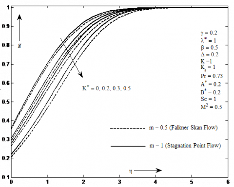
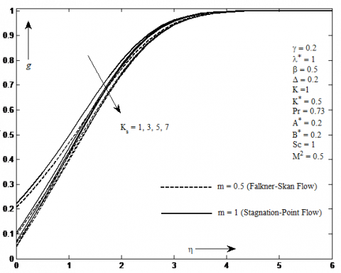
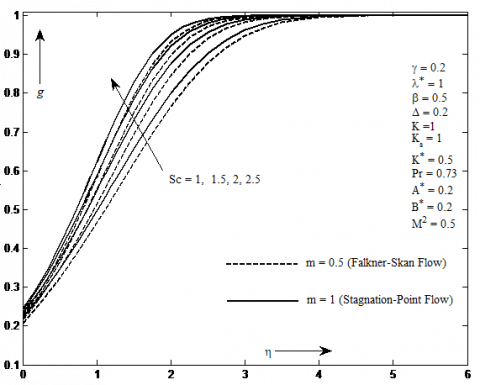
Figures 25-26 show the effects of intensity of the homogeneous reaction and heterogeneous reaction in concentration profile. As estimated that both parameters are reducing the concentration profile, that is concentration boundary layer profile decreases with homogeneous and heterogeneous reaction parameter. The concentration profile is lower for Falkner-Skan flow. Figure 27 describes the Schmidt number effects on species concentration profile, it reveals that Schmidt number is responsible for increases the species concentration profile.
Figure 24. Influence of inertia coefficient parameter on species concentration
Figure 25. Influence of homogeneous reaction strength on species concentration
Figure 26. Influence of heterogeneous reaction strength on species concentration
Figure 27. Influence of Schmidt number on species concentration
Tables 2 and 3 show the variation of the skin friction coefficient and Nusselt number for different parameters. We calculated these values for both stagnation-point flow and Falkner-Skan flow. The comparison is made between stagnation-point flow and Falkner-Skan flow for skin friction coefficient and Nusselt number.
Table 1. Comparison of f''(0) between existing results and present result
|
λ |
Rajagopal et al. (1983) |
Ishak et al. (2009) |
Jafar (2013) |
El-Dabe et al. (2009) |
Present study |
|
0.0 |
- |
0.4696 |
0.4696 |
0.4696007 |
0.469600085 |
|
0.1 |
0.587035 |
0.5870 |
0.5871 |
0.5870358 |
0.587035325 |
|
0.3 |
0.774755 |
0.7748 |
0.7748 |
0.7747554 |
0.774754891 |
|
0.5 |
0.927680 |
0.9277 |
0.9277 |
0.9276813 |
0.927679393 |
|
1.0 |
1.232585 |
1.2326 |
1.2326 |
1.2325901 |
1.232586607 |
Table 2. Skin friction coefficient for various parameters when Pr=0.73
|
M2 |
β |
γ |
K |
Δ |
λ* |
$\left( 1 + \frac { 1 } { \beta } \right) f ^ { \prime \prime } ( 0 )$ Stagnation-Point Flow (m = 1) |
$\left( 1 + \frac { 1 } { \beta } \right) f ^ { \prime \prime } ( 0 )$ Falkner-Skan Flow (m = 0.5) |
|
0.5 |
0.5 |
0.2 |
1 |
0.2 |
1 |
0.216846979 |
0.182734153 |
|
0.7 |
|
|
|
|
|
0.195144647 |
0.155805855 |
|
0.9 |
|
|
|
|
|
0.172216398 |
0.127338086 |
|
|
1 |
|
|
|
|
0.395175351 |
0.333383799 |
|
|
1.5 |
|
|
|
|
0.517596306 |
0.436951324 |
|
|
|
-0.2 |
|
|
|
0.311447254 |
0.270759332 |
|
|
|
0.3 |
|
|
|
0.189456522 |
0.157451669 |
|
|
|
|
10 |
|
|
0.507178899 |
0.494345054 |
|
|
|
|
100 |
|
|
1.545461237 |
1.541616465 |
|
|
|
|
|
0.4 |
|
0.231734653 |
0.200201758 |
|
|
|
|
|
0.6 |
|
0.245783529 |
0.216372194 |
|
|
|
|
|
|
1.5 |
0.215108456 |
0.181711443 |
|
|
|
|
|
|
2 |
0.213892326 |
0.180990580 |
Table 3. Nusselt for various parameters when Pr = 0.73
|
M2 |
β |
γ |
K |
Δ |
λ* |
A*=B* |
$- \theta ^ { \prime } ( 0 )$ Stagnation-Point Flow (m = 1) |
$- \theta ^ { \prime } ( 0 )$ Falkner-Skan Flow (m = 0.5) |
|
0.5 |
0.5 |
0.2 |
1 |
0.2 |
1 |
0.2 |
0.385893105 |
0.380462958 |
|
0.7 |
|
|
|
|
|
|
0.386158762 |
0.388098070 |
|
0.9 |
|
|
|
|
|
|
0.386859598 |
0.397685690 |
|
|
1 |
|
|
|
|
|
0.386462671 |
0.376883541 |
|
|
1.5 |
|
|
|
|
|
0.386888817 |
0.375506758 |
|
|
|
-0.2 |
|
|
|
|
0.376067020 |
0.397721569 |
|
|
|
0.3 |
|
|
|
|
0.388988339 |
0.377356696 |
|
|
|
|
10 |
|
|
|
0.391265785 |
0.361083721 |
|
|
|
|
100 |
|
|
|
0.403180770 |
0.354619607 |
|
|
|
|
|
0.4 |
|
|
0.386032465 |
0.377829572 |
|
|
|
|
|
0.6 |
|
|
0.386208647 |
0.375693322 |
|
|
|
|
|
|
1.5 |
|
0.386157653 |
0.380994161 |
|
|
|
|
|
|
2 |
|
0.386430090 |
0.381459589 |
|
|
|
|
|
|
|
0.4 |
0.362368213 |
0.398444090 |
|
|
|
|
|
|
|
0.6 |
0.379828298 |
0.455817741 |
We have considered a steady, laminar, two-dimensional boundary layer Casson fluid flow of a hydromagnetic coupled heat transfer on a moving plate and a moving wedge with variable induced magnetic field porous medium, second order resistance, non-uniform heat source and homogeneous-heterogeneous reactions. Some essential results are as follows:
(i) Velocity profile and induced magnetic profile decreases with magnetic field parameter and reciprocal magnetic Prandtl number, while increasing with Casson fluid parameter moving wedge/plate parameter, permeability parameter and inertia coefficient parameter. In all results, trends of stagnation-point flow is higher than Falkner-Skan flow.
(ii) Temperature profile reduces for the Casson fluid parameter, moving wedge/plate parameter, permeability parameter and inertia coefficient parameter, moreover temperature profile shows enhancement for magnetic field parameter and heat source parameter. It is noticed that the temperature profile is higher for stagnation-point flow when we compare it with Falkner-Skan flow.
(iii) Species concentration profile shrinks with magnetic field parameter, homogeneous reaction strength parameter and heterogeneous reaction strength parameter, furthermore concentration profile is the increasing function of Casson fluid parameter, permeability parameter, inertia coefficient parameter and Schmidt number. It is observed that Falkner-Skan flow is lower than stagnation-point flow.
Abbas Z., Sheikh M., Pop I. (2015). Stagnation-point flow of a hydromagnetic viscous fluid over stretching/shrinking sheet with generalized slip condition in the presence of homogeneous heterogeneous reactions. J Taiwan Inst Chem Engrs, Vol. 55, pp. 69-75. https://doi.org/10.1016/j.jtice.2015.04.001
Ali F. M., Nazar R., Arifin N. M., Pop I. (2011). MHD mixed convection boundary layer flow toward a stagnation point on a vertical surface with induced magnetic field was studied. J. Heat Transf., Vol. 133, pp. 1-6. https://doi.org/10.1115/1.4002602
Ali K., Ashraf M., Ahmad S., Batool K. (2012). Viscous dissipation and radiation effects in MHD stagnation point flow towards a stretching sheet with induced magnetic field. World Appl. Sci. J., Vol. 16, pp. 1638-1648.
Animasaum I. L., Raju C. S. K., Sandeep N. (2016). Unequal diffusivities case of homogeneous-heterogeneous reactions within viscoelastic fluid flow in the presence of induced magnetic field and nonlinear thermal radiation. Alexandria Eng. J., Vol. 55, pp. 1595-1606. https://doi.org/10.1016/j.aej.2016.01.018
Bayat R., Rahimi A. B. (2017). Numerical solution of three-dimensional N-S equations and energy in the case of unsteady stagnation-point flow on a rotating vertical cylinder. Int. J. Therm. Sci., Vol. 118, pp. 386-396. https://.doi.org/10.1016/j.ijthermalsci.2017.05.007
Casson N. (1959). Rheology of dispersed system. In: Mill CC. editor. Oxford: Pergamon Press.
Chaudhary M. A., Merkin J. H. (1995). A simple isothermal model for homogeneous-heterogeneous reactions in boundary-layer flow I. Equal diffusivities. Fluid Dyn Res., Vol. 16, pp. 311-333.
Chauhan D. S., Agrawal R. (2011). MHD flow and heat transfer in a channel bounded by a shrinking sheet and a plate with a porous substrate. J. Eng. Phys. Thermophysics, Vol. 84, No. 5, pp. 1034-1046. https://doi.org/10.1007/s10891-011-0564-y
Chauhan D. S., Rastogi P. (2011). Heat transfer and entropy generation in MHD flow through a porous medium past a stretching sheet. Int. J. Energy & Tech., Vol. 3, No. 15, pp. 1-13.
Chiam T. C. (1994). Stagnation-point flow towards a stretching plate. J Phys. Soc. Jpn., Vol. 63, pp. 2443-2444. https://doi.org/10.1143/JPSJ.63.2443
El-Dabe N. T., Ghaly A. Y., Rizkallah R. R., Ewis K. M., Al-Bareda A. S. (2015). Numerical solution of MHD boundary layer flow of non-Newtonian Casson fluid on a moving wedge with heat and mass transfer and induced magnetic field. J. Appl. Math. & Phys., Vol. 3, pp. 649-663. https://doi.org/10.4236/jamp.2015.36078
Falkner V. M., Skan S. W. (1931). Some approximate solutions of the boundary layer equations. Philos. Mag., Vol. 12, pp. 865-896. https://doi.org/10.1080/14786443109461870
Ganapathirao M., Ravindran R., Momoniat E. (2016) Effects of chemical reaction, heat and mass transfer on an unsteady mixed convection boundary layer flow over a wedge with heat generation/absorption in the presence of suction or injection. Int. J. Heat Mass Transf., Vol. 51, pp. 289-300. https://doi.org/10.1007/s00231-014-1414-1
Gireesha B. J., Mahanthesh B., Shivakumara I. S., Eshwarappa K. M. (2016). Melting heat transfer in boundary layer stagnation-point flow of nanofluid toward a stretching sheet with induced magnetic field. Eng. Sci. & Tech., Vol. 19, pp. 313-321. https://doi.org/10.1016/j.jestch.2015.07.012
Ishak A., Jafar K., Nazar R., Pop I. (2009). MHD stagnation point flow towards a stretching sheet. Physica A., Vol. 388, pp. 3377-3838. https://doi.org/10.1016/j.physa.2009.05.026
Ishak A., Nazar R., Pop I. (2009). MHD Boundary Layer Flow past a Moving Wedge. Magnetohydrodynamics, Vol. 45, pp. 3-10.
Jafar K., Nazar R., Ishak A., Pop I. (2013). MHD Boundary Layer Flow Due to a Moving Wedge in a Parallel Stream with the Induced Magnetic Field. Boundary Value Problems., Vol. 2013, pp.1-14. https://doi.org/10.1186/1687-2770-2013-20
Jain S., Bohra S. (2016). Radiation Effects in Flow through Porous Medium over a Rotating Disk with Variable Fluid Properties. Adv. Math. Phys., Vol. 2016, pp. 1-12. https://doi.org/10.1155/2016/9671513
Jain S., Choudhary R. (2015). Effects of MHD on boundary layer flow in porous medium due to exponentially shrinking sheet with slip. Procedia Engineering, Vol. 127, pp. 1203-1210. https://.doi.org/10.1016/j.proeng.2015.11.464
Kasmani R. M., Sivasankaran S., Bhuvaneswari M., Siri Z. (2016). Effects of chemical reaction on convective heat transfer of boundary layer flow in nanofluid over a wedge with heat generation/absorption and suction. J. appl. Fluid Mechanics, Vol. 9, No. 1, pp. 379-388. https://doi.org/10.18869/acadpub.jafm.68.224.24151
Khan M. I., Hayat T., Khan M. I., Alsaedi A. (2017). A modified homogeneous-heterogeneous reaction for MHD stagnation flow with viscous dissipation and Joule heating. Int. J. Heat Mass Transf., Vol. 113, pp. 310-317. https://.doi.org/10.1016/j.ijheatmasstransfer.2017.05.082
Khan M., Azam M., Alshomrani A. S. (2017). Effects of melting and heat generation/absorption on unsteady Falkner-Skan flow of Carreau nanofluid over a wedge. Int. J. Heat Mass Transf., Vol. 110, pp. 437-446. https://doi.org/10.1016/j.ijheatmasstransfer.2017.03.037
Lin H. T., Lin L. K. (1987). Similarity solutions for laminar forced convection heat transfer from wedges to fluids of any Prandtl number. J. Heat Mass Transf., Vol. 30, pp. 1111-1118. https://doi.org/10.1016/0017-9310(87)90041-X
Merkin J. H. (1996). A model for isothermal homogeneous–heterogeneous reactions in boundary-layer flow. Math Comput Model, Vol. 24, pp. 125-136. https://doi.org/10.1016/0895-7177(96)00145-8
Mukhopadhyay S., Ranjan D. P., Bhattacharyya K., Layek G. C. (2013). Casson fluid flow over an unsteady stretching surface. Ain Shams Eng. J., Vol. 4, pp. 933-938. https://doi.org/10.1016/j.asej.2013.04.004
Pramanik S. (2014). Casson fluid flow and heat transfer past an exponentially porous stretching surface in presence of thermal radiation. Ain Shams Eng. J., Vol. 5, pp. 205-212. https://doi.org/10.1016/j.asej.2013.05.003
Rajagopal K. R., Gupta A. S., Nath T. Y. (1983) A Note on the Falkner-Skan Flows of a Non-Newtonian Fluid. Int. J. Non-Linear Mech., Vol. 18, pp. 313-320. https://doi.org/10.1016/0020-7462(83)90028-8
Raju C. S. K., Sandeep N. (2017). MHD slip flow of a dissipative Casson fluid over a moving geometry with heat source/sink: A numerical study. Acta Astronautica. Vol. 133, pp. 436-443. https://doi.org/10.1016/j.actaastro.2016.11.004
Raptis A., Perdikis C. (1984). Free Convection under the Influence of a Magnetic Field. Nonlinear Anal.: Theory, Methods & Appl., Vol. 8, pp. 749-756. https://doi.org/10.1016/0362-546X(84)90073-7
Srinivasacharya D., Shafeeurrahman M. (2017). Joule heating effect on entropy generation in MHD mixed convection flow of chemically reacting nanofluid between two concentric cylinders. International Journal of Heat and Technology, Vol. 35, No. 1, pp. 487-497. https://doi.org/10.18280/ijht.350305
Wang C. Y. (2008). Stagnation flow towards a shrinking sheet. Int. J. Nonlin. Mech., Vol. 43, pp. 377-382. https://doi.org/10.1016/j.ijnonlinmec.2007.12.021