OPEN ACCESS
This study analyses the modelling and simulation of different hybrid electric vehicles(HEV) from battery, DC to DC converter, electric motor and generator, operational modes, planetary gear, internal combustion engine, vehicle body, vehicle dynamics, and control system. Several HEVs are simulated based on different size on specific drive cycle, and fuel consumption is recorded for each. The optimized HEV is extracted from regression model calculated by MATLAB with different polynomial order.
regression analyses, fuel consumption, optimal model, hybrid electric vehicle, drive cycle
This article investigates the modelling and simulation of different hybrid electric vehicles (HEV). All HEVs components are included to design a holistic scheme of real vehicle. This model is included, battery, DC to DC converter, electric motor and generator, operational modes, planetary gear, internal combustion engine, vehicle body, vehicle dynamics, and control system. Eight different hybrid electric vehicles on ten different standardized tire sizes are simulated for their fuel consumption on an urban dynamometer driving schedule UDDS FTP75. Fuel consumption data from those eighty simulations are recorded and processed in different regression analyses to find out the best fit model to estimate the fuel consumption and to determine the optimal vehicle size and tire for the best fuel economy. Finally fuel consumptions are simulated on several other drive cycles of FTP75, NYCC, HWFET, and EUDC for comparison of the optimized model and the nearby model.
Hybrid vehicle is a vehicle with at least two power sources, typically one of the power sources is provided by an electrical motor. Hybrid electrical vehicles (HEVs) are the type of hybrid vehicle that combines the best merits of internal combustion engine (ICE) and electric motor (EM). Hybrid Vehicles can save up to 45% less fuel when compared to conventional vehicle in the same class.
These are three main types of HEVs: series, parallel, and the series-parallel. In series type the internal combustion engine is not connected to the vehicle powertrain and it only is used to rotate the generator to provide electrical power to battery. The electrical power from the battery is used to propel the wheels. In the parallel type mechanical and electrical power are both connected to the powertrain of the vehicle and different control strategies are used during motion to determine if only the EM is used (at low speed) or if only the ICE is used (at high speed) or if both the ICE and EM are used to run the wheels in very high speed or extreme load. In the series-parallel type, it is like the parallel type but has an additional electric motor and a planetary gear unit, this makes the control complex but more efficient as one of the electric motor runs as a generator for charging the battery while the other is used for the running the wheel.
Reviewing some recent researches on HEVs fuel economy modeling and simulations: Simulations and design of HEV dual clutch transmission is referred in (Minh et al., 2017; Afzulpurkar, 2018), where three HEV models are designed and simulated in different driving cycles for achieving the optimal fuel saving; A research of optimization with multi objective for HEV emissions and fuel economy with the self-adaptive differential evolution algorithm is found in (Wu et al., 2011); Optimization of HEV management energy strategy based on some driving cycle modeling is presented in (Naxin & Shim, 2015; Cui et al., 2015) to increase the fuel economy and management for HEVs. Advanced control technologies are applied into the fuel saving control. A control strategy based on fuzzy controller optimized by Sugeno and Mamdani optimization is presented in (Minh et al., 2016; Reza & Minh, 2016); Fuel management economy for HEV and battery modeling can be controlled is introduced in (Liu, 2013). Fuzzy logic control of clutch vibration of HEV is designed in (Minh & Pumwa, 2013), and model predictive controller for real-time power strategy transmission for HEV is found in (Minh & Hashim, 2012). Effective torque of brake allocation in braking regenerative system for vibration in shaft with model predictive control is presented in (Naik & Shim, 2015). In a comprehensive scheme, ooperations of electric vehicle traction system has been reviewed by Youssef in (Youssef, 2018).
In our paper, a high-level model of HEV is built and simulated for eight (8) different HEVs using ten (10) different tire sizes in a typical city driving cycle FTP75. Eighty (80) data of fuel consumptions are recorded and processed in different regression models to find out the best fit model to predict the HEV fuel consumption and to generate the optimal HEV size for best fuel economy performance. Lastly, several simulations of fuel consumption between the optimal HEV and the nearby HEV are conducted on several drive cycles to compare their fuel consumption performances. The layout of this paper is as follows: Section 2 briefs HEV modelling; Section 3 presents fuel economy regression model analyses, HEVs simulations and comparison; and finally, Section 4 draws conclusions and recommendations.
2.1. Battery
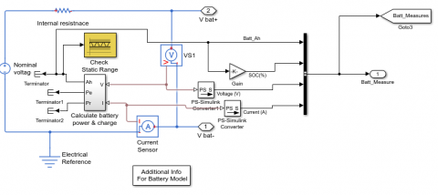
The battery is modeled as resistance and voltage which changes the load and power flow. A sub-block was modeled for the state of charge (SOC) taking voltage and current as input and the output of the battery voltage is just over 200V is connected to the input of the DC to DC converter. The modeling criteria used for the battery model can be found in (Liu, 2013) and shown in Figure 1.
The differential equation for electrical scheme is
$\frac { d V _ { \text {terminal} } } { d t } + \frac { V _ { \text {terminal} } } { R _ { d y } C _ { d y } } = R _ { \text {ohm} } \frac { d I } { d t } + \frac { R _ { d y n } + R _ { \text {ohm} } } { R _ { d y n } C _ { d y n } } I + \frac { V _ { o c } } { R _ { d y n } C _ { d y n } }$ (1)
where I is the terminal current of the battery (A), Vterminal is the battery system terminal voltage (V), T is the battery temperature, and Voc, Rohm, Rdyn, and Cdyn are the scheme parameters which depend on T and SOC.
Battery calculation of SOC can be applied from the integration of current:
$\operatorname { SOC } ( t ) = \operatorname { SOC } \left( t _ { i } \right) + \frac { 1 } { \operatorname { Cap } _ { A h r } 3600 } \int _ { t _ { i } } ^ { t } I ( t ) \eta _ { b a t } ( \operatorname { SOC } , T , \operatorname { sign } [ I ( t ) ] ) d t$ (2)
where $\eta _ { b a t }$ is the efficiency battery Coulombic and CapAhr is the ampere-hours capacity.
Figure 1. Battery in simulink model
2.2. DC-DC converter
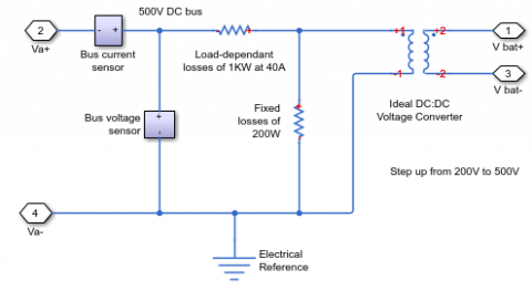
The DC - DC converter is seen as DC equivalent to a transformer AC with a continuously turning ratio. Like a transformer, it is used to step up or step-down DC voltage source. The criteria used for the modelling of the DC-DC converter can be found in (Minh & Pumwa, 2013) and (Minh & Hashim, 2012). For this study the DC to DC converter is used to boost the input voltage from 200V to the output voltage of 500V to drive the motor. The Simulink model of DC-DC converter is drawn in Figure 2.
Figure 2. DC - DC converter in Simulink model
The mathematical relationship used for modelling the DC - DC converter
Voltage transformation ratio $= \frac { N _ { \text {Secondary } } } { N _ { \text {Primary } } } = \frac { V _ { \text {Secondary } } } { V _ { \text {Primary } } }$ (3)
where V is voltage and N is the number of winding in turns. A transformer to increase the voltage from primary to secondary is named step-up transformer. A transformer produced to reduce voltage from primary to secondary is named step-down transformer. The ratio of transformation for a transformer being equal to the square rooted of inductance (L) primary to secondary ratio.
2.3. Electrical motor and generator model
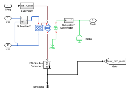
The servomotor is used to represent the generator and the electrical motor, the required output torque is tracked from the torque demand reference from the control system. Both the servo motor and servo generator are connected to the DC supply. The function of the electrical motor is to supply torque to the transmission required for the propelling of the vehicle, while the generator is used to start the combustion engine and to charge the HEV battery through regenerative braking at certain mode in the control process. Criteria used for modeling the motor can be referred in (Liu, 2013) and generator can be referred in (Naik & Shim, 2015). Figure 3 and Figure 4 show the Simulink model of the electrical motor and generator, the blue lines in both figures indicate the electrical part of the model while the green parts indicate the mechanical system.
Figure 3. Motor in Simulink model
Figure 4. Generator in Simulink model
Three operational modes of motor and generator are as follows:
2.3.1. Operation of propulsion mode
When an electrical motor runs in this mode, it supplies the propulsion torque, and its behavior is depicted from following equations:
$\tau _ { \mathrm { mot } } = \tau _ { \mathrm { demand } } + \tau _ { \mathrm { spin } _ { \mathrm { loss } } } + J _ { \mathrm { mot } } \frac { \mathrm { d } \omega } { \mathrm { dt } } ( \text {output torque} )$ (4)
$\tau _ { m o t } \leq \max \left( \tau _ { m o t } \right) = f ( \omega ) ( \text {contrain } )$ (5)
$\tau _ { \text {spin } _ { \text {loss } } } = \alpha _ { 1 } \delta ( t ) + \alpha _ { 2 } \omega + \alpha _ { 3 } \operatorname { sgn } ( \omega ) ( \text {loss spin torque} )$ (6)
$\mathrm { P } _ { \text {elec } } = \frac { \mathrm { P } _ { \text {mech } } } { \mathrm { n } _ { \text {mot } } } = \frac { \tau _ { \text {mot } . \omega } } { \eta \left( \tau _ { \text {mot } , \omega } \right) }$ (required electrical power) (7)
$\eta _ { \mathrm { mot } } = \eta \left( \tau _ { \mathrm { mot } } , \omega \right) ( \text {motor efficiency} )$ (8)
$V _ { \text {mot } } = V _ { \text {bus } } ( \text { motor voltage } )$ (9)
$I _ { \operatorname { mot } } = \frac { P _ { \text {elec} } } { V _ { \text {bus} } } ( \text {motor required current} )$ (10)
where Jmot is the inertia of motor, $\tau_{mot}$ is the torque propulsion delivered by the electrical motor (Nm),
is the torque lost due to the friction (Nm), $\tau_{spin_loss}$ is the torque demanding from the HEV (Nm), $\tau_{demand}$ is the angular velocity of motor (rad/s), $max(\tau_{mot})=f(\omega)$ is the physical maximum torque of motor, α1, α2, and α3 are the static coefficient friction, viscous coefficient friction, and friction Coulomb coefficient, respectively, $\eta_{mot}$ is the efficiency lumped of the electrical motor, controller and inverter. Vbus is the bus high-voltage.2.3.2. Operation in regenerative mode
When an electrical motor runs in the regenerative mode, the generator supplies charge for the battery and provides negative (brake) torque for the vehicle. In this mode, the generator behavior can be determined by the following equations.
$\left| \tau _ { \text {regen } } \right| = \left| \tau _ { \text {demand } } \right| - \tau _ { \text {spin } _ { \text {- } } \text { loss } } + J _ { \text {mot } } \frac { \mathrm { d } \omega } { \mathrm { dt } } ( \text { brake torque } )$ (11)
$\left| \tau _ { \text {regen } } \right| \leq \max \left( \tau _ { \text {regen } } \right) = g ( \omega ) ( \text { contrain } )$ (12)
$\tau _ { \text {spin } \text{_} { \text {loss } } } = \alpha _ { 1 } + \alpha _ { 2 } \omega + \alpha _ { 3 } \operatorname { sgn } ( \omega ) ( \text {lost spin torque} )$ (13)
$\mathrm { P } _ { \text {elec } } = \eta _ { \text {regen } } \mathrm { P } _ { \text {mech } } = \eta \left( \tau _ { \text {regen } } , \omega \right) \tau _ { \text {regen } } \omega ( \text { general electrical power } )$ (14)
$\eta _ { \operatorname { mot } } = \eta \left( \tau _ { \text {regen } } , \omega \right) ( \text { motor efficiency } )$ (15)
$\mathrm { V } _ { \mathrm { mot } } = \mathrm { V } _ { \mathrm { bus } } ( \text {motor voltage} )$ (16)
$\mathrm { I } _ { \text {regen } } = \frac { \mathrm { P } \text { elec } } { \mathrm { V } _ { \text {bus } } } ( \text { generated current } )$ (17)
where Jmot is the inertia of motor, $\tau_{regen}$ is the negative brake motor torque (Nm), $\tau_{demand}$ is the torque demanding from the HEV (Nm), ω is the angular velocity of motor (rad/s), $max(\tau_{regen})$ is the maximum motor regenerative torque, and $\eta_{mot}$ is the regenerative efficiency lumped of the electrical motor, controller and inverter.
2.3.3. Operation in spinning mode
When an electrical motor runs in this mode, it is passively spun and supplies a minor negative torque friction for the HEV as:
$\tau _ { m o t } = \tau _ { s p i n _ { - } l o s s } = \alpha _ { 1 } \delta ( t ) + \alpha _ { 2 } \omega + \alpha _ { 3 } \operatorname { sgn } ( \omega )$ (18)
where $\tau_{mot}$ is the output torque, $\tau_{spin_loss}$ is the loss spin torque, α1, α2, and α3 are the static friction viscous friction coefficient, coefficient, and friction Coulomb coefficient on electrical motor and generator.
2.4. Planetary gear (power split)
Planetary gear is used in the series parallel HEV configuration for power split functionality between the mechanical (ICE) and the electrical link (Electrical Motor). The planetary gear connects the gasoline engine, generator and electric motor together allowing the vehicle to operate at different mode (ICE, Motor, ICE and Motor combine). The set of planetary gear (Power Split) includes of the sun gear, carrier, ring gear, and several pinion gears, carrier. The planetary gear scheme is drawn in Figure 5.
Figure 5. Planetary gear in Simulink model
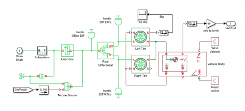
2.5. Vehicle dynamics
The vehicle dynamics is consisted of gear box, differential, left and right tires, and vehicle body. The vehicle body model is drawn in Figure 6.
Figure 6. Simulink model of vehicle body model
The HEV body provides the resistance rolling and aero-drag resistance forces of the HEV. The retarding forces of the HEV when the motionless is set equal to $F _ { \text {fric} } + F _ { \text {grade} }$. The propulsion force required at the given speed is presented by the relationship below.
$\mathrm { F } _ { \mathrm { wh } } = \mathrm { F } _ { \mathrm { rolling } } + \mathrm { F } _ { \mathrm { aero } } + \mathrm { F } _ { \mathrm { grade } } + \mathrm { m } _ { \mathrm { v } } \mathrm { a }$ (19)
where, Fwh is the force traction on the wheel by the powertrain, mv is the mass (kg), a is the HEV acceleration (m/s2), and $F _ { \text {rolling} } , F _ { \text {aero} } , F _ { \text {grade} }$ are resistance rolling, aero drag resistance, and weighing forces, respectively, expressed as:
$\mathrm { F } _ { \text {rolling } } \approx \mathrm { k } _ { \mathrm { rrc } } \mathrm { k } _ { \mathrm { sc } } \mathrm { m } _ { \mathrm { v } } \mathrm { g }$ (20)
$\mathrm { F } _ { \text {aero } } = \mathrm { k } _ { \text {aero } } \mathrm { V } ^ { 2 }$ (21)
$\mathrm { k } _ { \text {aero } } = \frac { 1 } { 2 } \mathrm { C } _ { \mathrm { a } } \mathrm { A } _ { \mathrm { d } } \quad \mathrm { C } _ { \mathrm { d } } \mathrm { F } _ { \mathrm { a } }$ (22)
$F _ { \text {grade} } = m _ { v } g \sin ( \alpha )$ (23)
where krrc is the resistance rolling coefficient, ksc is the coefficient of road surface, kaero is the factor aero drag, Ca is the density of air correction at the given altitude, Ad is air density of mass (km/m3), Cd is the drag aerodynamic coefficient of HEV (N $\frac{s^2}{kg}$ m), Fa is the area frontal of HEV (m2), and α is the incline angle of road (rad).
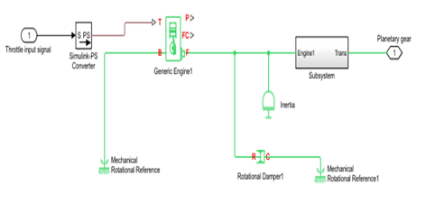
2.6. Internal combustion engine
The engine generates driving torque of $T _ { e } \left( \omega _ { e } , x _ { \theta e } \right)$ and the gearbox applies Tg as the load to the engine. The equation of the engine rotational motion can then be formulated as:
$\mathrm { T } _ { \mathrm { e } } \left( \omega _ { \mathrm { e } } , \mathrm { x } _ { \theta \mathrm { e } } \right) - \mathrm { T } _ { \mathrm { g } } = \mathrm { I } _ { \mathrm { e } }\frac{d_{\omega e}}{dt}$ (24)
where $\omega _ { e } , x _ { \theta e }$ and $I _ { e }$ are engine rotational speed, throttle position, and equivalent rotational inertia of engine respectively. While $x _ { \theta e }$ is assume as a variable in the range of [0%–100%]. The vehicle engine scheme is drawn in Figure 7.
Figure 7. Vehicle engine in Simulink model
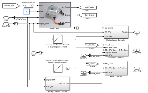
2.7. Control system
The control system is designed from five separated sub blocks namely: Motor Controller; Mode Logic; Battery Controller; Generator Controller; and Engine Controller. The system control performs decisions required for the control of the HEV and drawn in Figure 8.
Figure 8. Control system in Simulink model
Based on the high-level Simulink mode of HEV, eight (8) different HEVs on ten (10) different standardized tire sizes are selected to simulate for 100 seconds on the typical urban driving cycle FTP75. Table 1 shows the data of 8 vehicle curb weights (curb weight is the authentic weight of a vehicle including all the factory-installed equipment, facilities, and 90% full fuel tank).
Table 1. Vehicle curb weights
|
No |
Car model and year |
Curb weight Kg |
|
1 |
Toyota Prius (2009-2015) |
1325 (Toyota, 2015) |
|
2 |
Honda Insight Hybrid (2009-2014) |
1237 (Honda, Honda Insight, 2014) |
|
3 |
Kia Niro Hybrid (2016) |
1409 (Kia, 2016) |
|
4 |
Hyundai Sonata Hybrid (2011-2013) |
1568 (Hyundai, 2014) |
|
5 |
Kia Optima Hybrid (2016) |
1585 (KiaOpti, 2016) |
|
6 |
Hyundai Avante LPi Hybrid |
1297 (HyundaiCat, 2010) |
|
7 |
Toyota Camry Hybrid (2007) |
1649 (CamryHybrid, 2015) |
|
8 |
Honda Civic hybrid (2011-2016) |
1280 (Honda, Honda Civic Hybrid, 2016) |
And Table 2 shows the 10 different standardized tires that are able to install into those vehicles (Errolstyres, 2016):
Table 2. Tire sizes with rolling radius
|
No |
Tires size |
Rolling radius M |
Recommended rim Inch |
|
1 |
155/65 R13 |
0,241 |
4,5 |
|
2 |
155/80 R13 |
0,261 |
4,5 |
|
3 |
165/60 R14 |
0,251 |
5,0 |
|
4 |
165/65 R13 |
0,247 |
5,0 |
|
5 |
165/65 R14 |
0,258 |
5,0 |
|
6 |
165/70 R14 |
0,266 |
5,0 |
|
7 |
165/80 R13 |
0,269 |
4,5 |
|
8 |
175/65 R14 |
0,264 |
5,0 |
|
9 |
175/65 R15 |
0,276 |
5,0 |
|
10 |
205/50 R15 |
0,277 |
6,5 |
Results of fuel consumption data for 80 simulations of different eight HEVs on different ten tire sizes for 100 seconds over the driving cycle FEP75 are shown in Table 3.
Table 3. Fuel consumption (liter/s) (weight kg (W) Vs Rolling radius m (R))
|
W |
1325 |
1237 |
1409 |
1568 |
1585 |
1297 |
1649 |
1280 |
|
R |
||||||||
|
0.241 |
0.01984 |
0.01984 |
0.01985 |
0.01993 |
0.01995 |
0.01984 |
0.02009 |
0.01984 |
|
0.261 |
0.01961 |
0.01961 |
0.01964 |
0.02032 |
0.02052 |
0.01961 |
0.02181 |
0.01961 |
|
0.251 |
0.01973 |
0.01973 |
0.01973 |
0.0199 |
0.01995 |
0.01973 |
0.02053 |
0.01973 |
|
0.247 |
0.01977 |
0.01977 |
0.01977 |
0.01991 |
0.01993 |
0.01997 |
0.02024 |
0.01977 |
|
0.258 |
0.01966 |
0.01964 |
0.01968 |
0.01995 |
0.02025 |
0.01964 |
0.02121 |
0.01964 |
|
0.266 |
0.01956 |
0.01957 |
0.01957 |
0.02057 |
0.02088 |
0.01957 |
0.02255 |
0.01957 |
|
0.269 |
0.01953 |
0.01954 |
0.01959 |
0.02091 |
0.02129 |
0.01953 |
0.02322 |
0.01954 |
|
0.264 |
0.01958 |
0.01959 |
0.01962 |
0.02045 |
0.02063 |
0.01958 |
0.02209 |
0.01958 |
|
0.276 |
0.01948 |
0.01948 |
0.01956 |
0.02188 |
0.02238 |
0.01947 |
0.02511 |
0.01947 |
|
0.277 |
0.01962 |
0.01962 |
0.01965 |
0.02025 |
0.02046 |
0.01962 |
0.0216 |
0.01962 |
Fuel consumption data is processed on several regression analyses to find out the best fit regression model to estimate the fuel consumption for HEVs. Matlab supports calculation of the best fit regression via several equation orders.
$\text {Fuel consumption } \boldsymbol { F } = \text { function (Vehichle weight } \boldsymbol { W } , \text { and Tire radius } \boldsymbol { T } )$ (25)
Regression model for the first equation order:
$F _ { 1 } = f _ { 1 } ( W , T ) = P _ { 00 } + P _ { 10 } W + P _ { 01 } T$ (26)
where F1 is the first order fuel consumption calculation, W is the vehicle Weight, T is Tire radius, coefficients are calculated as P00=0.02014; P10=0.0006671; P01=0.0002533; Coefficient of determination for this first regression model R-square = 0.5365.
Regression model for the second equation order:
$F _ { 2 } = f _ { 2 } ( W , T ) = P _ { 00 } + P _ { 10 } W + P _ { 01 } T + P _ { 20 } W ^ { 2 } + P _ { 11 } W T + P _ { 02 } T ^ { 2 }$ (27)
where F2 is the second order fuel consumption calculation, W is the vehicle Weight, T is Tire radius, coefficients are calculated as P00=0.01947; P10=0.0004895; P01=0.0002959; P20=0.0005423; P11=0.0004615; P02=0.0001365. Coefficient of determination for this second regression model R-square = 0.8876.
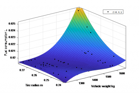
Regression model for the third equation order:
$\begin{aligned} F _ { 3 } = f _ { 3 } ( W , T ) & = P _ { 00 } + P _ { 10 } W + P _ { 01 } T + P _ { 20 } W ^ { 2 } + P _ { 11 } W T + P _ { 02 } T ^ { 2 } + \\ & + P _ { 30 } W ^ { 3 } + P _ { 21 } W ^ { 2 } T + P _ { 12 } W T ^ { 2 } + P _ { 03 } T ^ { 3 } \end{aligned}$ (28)
where F3 is the third order fuel consumption calculation, W is the vehicle Weight, T is Tire radius, coefficients are calculated as P00=0.01949; P10=-8.058e-05; P01=-8.597e-05; P20=0.0004236; P11=0.0004005; P02=0.0001392; P30=0.0003121; P21=0.0003402; P12=0.0001619; P03=2.071e-05. Coefficient of determination for this first regression model R-square = 0.9913.
Figure 10. Fuel consumption fit curve model for HEV
With the coefficient of determination R-square = 0.9913 or more than 99% of the fuel consumption being correctly calculated from the vehicle weight and tire radius, formula equation (28) is selected as the final decision to predict the fuel consumption on the city driving cycle FEP75. The third order relationship of vehicle weight (kg) and tire radius (meter) to the fuel consumption (liter) is shown in Figure 10.
Differentiation of equation (28) or $F _ { 3 } ^ { \prime } = f _ { 3 } \left( W ^ { \prime } T ^ { \prime } \right)$ with respect to W and T leads to an optimal first order linear equation for fuel consumption as follows
$3,0540 e ^ { - 6 } W + 0,0212 T - 0,0096 = 0$ (29)
Equation (29) allows calculating the optimal vehicle weights subject to the standardized tire rolling radius as shown tin Table 4
Table 4. Optimal vehicle weight subject to tire rolling radius
|
Tire Rolling radius (m) |
0.241 |
0.247 |
0.251 |
0.258 |
0.261 |
0.264 |
0.266 |
0.269 |
0.276 |
0.277 |
|
HEV optimal Wight (kg) |
1471 |
1429 |
1401 |
1353 |
1332 |
1311 |
1297 |
1276 |
1228 |
1221 |
In order to verify the optimal fuel consumption in equation (28) and (29), simulations are carried out on different drive cycles (FTP75, NYCC, HWFET, EUDC) for an optimal HEV having optimal weight of 1221 Kg with tire radius of 0.277 m to a lighter HEV of 1200 Kg using smaller tire radius of 0.261 m. Results of fuel consumptions are indicated in table 5.
Table 5. Comparison of fuel consumption between two HEVs
|
No |
Vehicle type |
Drive cycle |
Vehicle weight kg |
Tire rolling radius m |
Fuel consumed l/s |
|
1 |
HEV Optimal HEV |
FTP75 |
1200 1221 |
0,261 0.277 |
0,03668 0,03649 |
|
2 |
HEV Optimal HEV |
NYCC |
1200 1221 |
0,261 0,277 |
0,03295 0,03263 |
|
3 |
HEV Optimal HEV |
HWFET |
1200 1221 |
0,261 0,277 |
0,03969 0,03915 |
|
4 |
HEV Optimal HEV |
EUDC |
1200 1221 |
0,261 0,277 |
0,03715 0,03655 |
Table 5 shows that the fuel consumption of optimal vehicle is always less than the nearby lighter weight and smaller tire rolling radius vehicle.
This study successfully builds up a high-level modeling of HEV with battery, converter, electric motor and generator, planetary gear, internal combustion engine, vehicle body, vehicle dynamics and the control system for HEV. Different HEVs are selected with different weights to simulate the fuel consumption on different tire rolling radiuses. Results of fuel consumption are analyzed and processed on several regression models. The best regression model is the third order polynomial equation with more than 99% of the fuel consumption being able exactly estimated. The fuel consumption regression model helps to identify the HEVs optimal weight subject to their tire rolling radius. Results of HEV optimal weight vs tire radius are also re-verified by simulations of optimal HEV and non-optimal HEV. HEV designers can refer to this study to select their HEV parameter to achieve the best fuel economy performance.
The authors would like to thank Tallinn University of Technology (TalTech) for supporting this research project.
Afzulpurkar N. (2018). Automatic control of clutch engagement and slip for hybrid vehicle. International Journal of Innovative Technology and Interdisciplinary Sciences, Vol. 1, No. 1, pp. 49-61. http://doi.org/10.15157/IJITIS.2018.1.1.49-61
CamryHybrid. (2015). Camry Hybrid Features and Specs. Retrieved from https://www.errolstyres.co.za/content/tyre-overall-rolling-diameter
Cui N. X., Lian F. X., Wu J. C., Wang X. J. (2015). Optimization of HEV energy management strategy based on driving cycle modeling. China: 34th Chinese Control Conf. http://doi.org/10.1109/ChiCC.2015.7260908
Errolstyres. (2016). Tyre overall rolling diameter. Retrieved from https://www.errolstyres.co.za/content/tyre-overall-rolling-diameter
Honda. (2014). Honda Insight. Retrieved from https://en.wikipedia.org/wiki/Honda_Insight
Honda, Honda Civic Hybrid. (2016). Retrieved from https://en.wikipedia.org/wiki/Honda_Civic_Hybrid
Hyundai. (2014). HYUNDAI Sonata Hybrid 2010-2014. Retrieved from https://www.autoevolution.com/cars/hyundai-sonata-hybrid-2010.html#aeng_hyundai-sonata-hybrid-2010-24-blue-drive
HyundaiCat. (2010). Hyundai Catalogue. Retrieved from http://www.automobile-catalog.com/car/2010/1180580/hyundai_avante_lpi_hybrid.html
Kia. (2016). Kia niro specification. Retrieved from https://www.kiamedia.com/us/en/models/niro/2017/specifications
KiaOpti. (2016). Kia optima hybrid. Retrieved from https://www.kiamedia.com/us/en/models/optima-hybrid/2016/specifications
Liu W. (2013). Hybrid vehicle system modeling. Introduction to Hybrid Vehicle System Modeling and Control, pp. 432. http://doi.org/10.1002/9781118407400
Minh V., Hashim M. A. (2012). Development of a real-time clutch transition strategy for a parallel hybrid electric vehicle. Journal Syst and Control Eng, Vol. 226, No. 2, pp. 188-203. http://doi.org/10.1177/0959651811414760
Minh V., Pumwa J. (2013). Fuzzy logic and slip controller of clutch and vibration for hybrid vehicle. Int J Control Autom Syst, Vol. 11, No. 3, pp. 526-532. http://doi.org/10.1007/s12555-012-0006-4
Minh V., Ahmad M., Tamre M. (2017). Design and simulations of dual clutch transmission for hybrid electric vehicles. Int J Electr Hybrid Veh, Vol. 9, No. 4, pp. 302-321. http://doi.org/10.1504/IJEHV.2017.089873
Minh V., Moezzi R., Mart T., Oliver M., Martin J., Ahti P., Mart J. (2016). Performances of PID and different fuzzy methods for controlling a ball on beam. Open Engineering Journal, Vol. 6, No. 1, pp. 145-151. http://doi.org/10.1515/eng-2016-0018
Minh V., Sivitski A., Tamre M., Penkov I. (2015). Modeling and control strategy for hybrid electrical vehicle. In New Applications of Electric Drives, pp. 27-57. INTECH. http://doi.org/10.5772/61415
Naik B., Shim T. (2015). Effective brake torque allocation in regenerative braking system considering shaft vibration using model predictive control. ASME Dynamic Systems and Control Conference, pp. 1-7. http://doi.org/10.1115/DSCC2015-9996
Reza M., Minh V. T. (2016). Fuzzy logic control for non-linear model of the ball and beam system. Paper presented at the Proceedings of the International Conference of DAAAM Baltic "Industrial Engineering", pp. 60-65. Retrieved from www.scopus.com
Toyota. (2015). Prius/Specifications. Retrieved from https://en.wikibooks.org/wiki/Toyota_Prius/Specifications
Wu L., Wang Y., Yuan X., Chen Z. (2011). Multiobjective optimization of HEV fuel economy and emissions using the self-adaptive differential evolution algorithm. IEEE Trans Veh Technol, Vol. 60, No. 6, pp. 2458-2470. http://doi.org/10.1109/TVT.2011.2157186
Youssef M. A. (2018). Operations of electric vehicle traction system. Mathematical Modelling of Engineering Problems, Vol. 5, No. 2, pp. 51-57. http://doi.org/10.18280/mmep.050201