© 2018 IIETA. This article is published by IIETA and is licensed under the CC BY 4.0 license (http://creativecommons.org/licenses/by/4.0/).
OPEN ACCESS
This paper aims to enhance the performance of power generation system. To this end, the author transferred the brushless double fed induction generator (BDFIG) model into the CW synchronous speed frame, oriented the CW synchronous speed frame model to three kinds of CW quantities, and deduced and compared three kinds of BDFIG models with different control features. After that, several control systems with current-inner-loop and voltage-outer-loop were designed and compared for the three kinds of BDFIG models. One of the proposed control systems was verified through prototype experiment. It is concluded that the CW-current-oriented model is the simplest one and the physical quantity of orientation (CW current) is easy to control and measure. The control system using voltage and current dual closed-loops can achieve the PW voltage control goals and realize the current limitation. The BDFIG models were proved valid through the prototype experiment. It is concluded that the CW-current-oriented model is the simplest one and the physical quantity of orientation (CW current) is easy to control and measure. The control system using voltage and current dual closed-loops can achieve the PW voltage control goals and realize the current limitation. The BDFIG models were proved valid through the prototype experiment.
brushless double fed induction generator (BDFIG), power winding (PW), control winding (CW), field-orientation
The brushless double fed induction generator (BDFIG) has two three-phase windings in the stator (namely the power winding, PW, and the control winding, CW) and a special rotor winding. The CW can modify and control the rotor current induced by the PW, and thus achieve the variable speed constant frequency (VSCF) control without slip rings or brush gear. The special motor structure enables the BDFIG to meet high reliability and low maintenance requirements in the absence of a brush gear. In recent years, the BDFIG electric system has received the widespread attention in the academia (Willianson et al., 2002; McMahon et al., 2006; Prousalidis et al., 2005; Xiong and Wang, 2011).
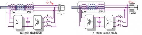
There are mainly two operation modes for the BDFIG: the grid-tied mode and the standalone mode. The former is mainly adopted for onshore wind power generation, and the latter for offshore wind power generation. In the grid-tied mode, the active power and reactive power from the PW are injected; In the standalone mode, the PW voltage is maintained as a constant.
Much research has been done on the grid-tied mode (Figure 1(a)). Since the PW is connected to the stable grid Vg, the PW flux or voltage orientation is often selected for the synchronous reference frame (Long et al., 2013; Poza et al., 2006; Poza et al., 2009; Liu et al., 2011) to achieve the vector control. This strategy meets new challenges in the standalone mode (Figure 1(b)). In this mode, the PW is directly connected to the load, such that the PW voltage phase and amplitude will be distorted by the load variation. The distortion of PW voltage will leave the field-oriented system uncorrected. To fix this problem, reference (Jiang et al., 2014) derives a mathematical model based on the PW and CW dual stationary frame system, and applies the model to study the direct torque control; reference (Zhang et al., 2011) controls the PW voltage in light of the static CW frame and the current orientation of the stator; reference (Chen et al., 2013) implements the direct torque control in the static frame system with a CW-based unified frame model.
The above analysis shows that the CW orientation must be considered for the standalone mode. Nevertheless, the previous studies often complicate the control system with either the stationary frame or the direct torque control. To overcome the problem, this paper the CW synchronous speed frame and the CW-quantities-orientation method for the BDFIG control in both the grid-tie and standalone modes.
The remainder of this paper is organized as follows: Section II transfers the BDFIG model into the CW synchronous speed frame; Section III further orients the CW synchronous speed frame model to three kinds of CW quantities, and deduces and compares three kinds of BDFIG models with different control features; Section IV designs and compares the control systems with current-inner-loop and voltage-outer-loop for the three kinds of BDFIG models; Section V verifies the effect of one of the proposed control systems through prototype experiment; Section VI wraps up this research with some meaningful conclusions.
In 2003, J. Poza deduced a BDFIG model, with which all the quantities can be transferred to any speed frame. The vector model is shown in the equation (1), where ωa is the random angular speed.
$\left\{\begin{array}{c}{v_{s 1}=R_{s 1} i_{s 1}+p \varphi_{s 1}+j \omega_{a} \varphi_{s 1}} \\ {\varphi_{s 1}=L_{s 1} i_{s 1}+L_{s 1 r} i_{r}} \\ {v_{s 2}=R_{s 2} i_{s 2}+p \varphi_{s 2}+j\left[\omega_{a}-\left(p_{1}+p_{2}\right) \omega_{r}\right] \varphi_{s 2}} \\ {\varphi_{s 2}=L_{s 2} i_{s 2}+L_{s 2 r} i_{r}} \\ {v_{r}=R_{r} i_{r}+p \varphi_{r}+j\left[\omega_{a}-p_{1} \omega_{r}\right] \varphi_{r}} \\ {\varphi_{r}=L_{s 1 r} i_{s 1}+L_{s 2 r} i_{s 2}+L_{r} i_{r}}\end{array}\right.$ (1)
If ωa is set to the PW angular speed ωp, the model is the PW orientation frame system and suitable for grid-tie mode (Shao et al., 2009).
$\left\{\begin{array}{c}{v_{s 1}=R_{s 1} i_{s 1}+p \varphi_{s 1}+j\left[\omega_{c}-\left(p_{1}+p_{2}\right) \omega_{r}\right] \varphi_{s 1}} \\ {\varphi_{s 1}=L_{s 1} i_{s 1}+L_{s 1 r} i_{r}} \\ {v_{s 2}=R_{s 1} i_{s 2}+p \varphi_{s 2}+j \omega_{c} \varphi_{s 2}} \\ {\varphi_{s 2}=L_{s 2} i_{s 2}+L_{s 2 r} i_{r}} \\ {v_{r}=R_{r} i_{r}+p \varphi_{r}+j\left[\omega_{c}-p_{2} \omega_{r}\right] \varphi_{r}} \\ {\varphi_{r}=L_{s 1 r} i_{s 1}+L_{s 2 r} i_{s 2}+L_{r} i_{r}}\end{array}\right.$ (2)
Figure 1. The diagram of two modes for the BDFIG
If ωa is set to the CW angular speed ωc, it is possible to obtain the model based on CW current orientation, as shown in equation (2).
Using this model, the CW angular speed ωc was calculated according to the inherent relationship between ωc, ω*p and ωr, where ω*p is the desired frequency of the PW voltage (50Hz or 60Hz). Since ωc is generated by the controller rather than the phase-locked loop, it is independent of the load variation and capable of ensuring system stability.
The vector equations in equation (2) were split into two parts in the d-q rotation reference frame with synchronous speed ωc. For further simplification of the BDFIG model, the d-axis of the reference frame was aligned to different CW quantities, such as the CW voltage vc, the CW flux φsc and the CW current ic. Different alignment methods resulted in different mathematical models. The derivations of three types of CW-quantities-orientation models are given below:
3.1. CW flux orientation
The conditions of CW flux orientation are:
$\varphi_{c d}=\varphi_{c} ; \varphi_{c q}=0$,Then, the relationship of PW voltage and CW current can be obtained as:
$v_{p d}=-\frac{s^{2} L_{s 1 r} L_{s 2 r}}{k_{r}} i_{c d}+$
$\underbrace{\frac{L_{s 1 r}\left(s L_{s 2 r}^{2} k_{r r}-s k_{r r} L_{r} L_{s c}+k_{p r} k_{r} L_{s c}\right)}{k_{r} L_{s 2 r}} i_{c q}+\frac{k_{p} k_{r}-s^{2} L_{s 1 r}^{2}}{k_{r}} i_{p d}+\frac{s k_{r r} L_{s 1 r}^{2}-k_{p r} k_{r} L_{s p}}{k_{r}} i_{p q}}_{k_{r}}$ (3)
$v_{p q}=\frac{k_{p r} L_{s 1 r} k_{r r} L_{s 2 r}^{2}-k_{p r} k_{r r} L_{s 1 r} L_{r} L_{s c}-s k_{r} L_{s 1 r} L_{s c}}{L_{s 2 r} k_{r}} i_{c q}$
$\underbrace{-\frac{s k_{p r} L_{s 1 r}}{k_{r}} i_{c d}+\frac{k_{p} k_{r}+k_{p r} k_{r r} L_{s 1 r}^{2}}{k_{r}} i_{p q}+\frac{k_{p r} L_{s p} k_{r}-s k_{p r} L_{s 1 r}^{2}}{k_{r}} i_{p d}}_{k_{r}}$ (4)
Hence, the orientation conditions are:
$i_{c d}=\frac{\Delta}{A(s)} v_{c d}-\frac{s L_{s 2 r}^{2} k_{s p} R_{r}}{A(s)} i_{c q}$ (5)
$i_{c q}=\frac{\Delta}{B(s)} v_{c q}+\frac{L_{s 2 r}\left(s k_{r}+k_{s r}^{2} L_{r}\right)+w_{c} L_{s c} R_{c} \Delta}{B(s)} i_{c d}$
$-\frac{w_{c} L_{s 2 r} L_{s l r}\left(s k_{r}+k_{s r}^{2} L_{r}\right)}{B(s)} i_{p d}+\frac{w_{c} L_{s 2 r} k_{s r} L_{s v r} R_{r}}{B(s)} i_{p q}$ (6)
where
$A(s)=-s^{2} L_{s 2 r}^{2} k_{r}+s k_{s r}^{2} L_{r}+k_{c} \Delta$
$B(s)=s L_{s c} \Delta-k_{p r} L_{s 2 r}^{2} \omega_{s} R_{r}$
3.2. CW voltage orientation
The conditions of CW flux orientation are:
vcd=vc;vcq=0.
Then, the relationship of PW voltage and CW current can be obtained as:
$\underbrace{\begin{align} & {{v}_{pd}}=\frac{{{s}^{3}}{{L}_{s1r}}{{k}_{c}}+{{s}^{2}}w_{c}^{2}{{L}_{s1r}}{{L}_{sc}}+s{{k}_{p}}{{L}_{s1r}}{{w}_{s}}{{k}_{c}}+{{k}_{p}}{{L}_{s1r}}w_{c}^{3}{{L}_{sc}}-{{k}_{p}}{{L}_{s1r}}{{w}_{c}}{{k}_{sc}}{{L}_{sc}}}{s{{L}_{s2r}}{{k}_{sc}}}{{i}_{cd}} \\ & +\frac{{{s}^{2}}{{L}_{s1r}}-{{k}_{p}}{{L}_{s1r}}{{w}_{c}}}{{{L}_{s2r}}{{k}_{sc}}}{{v}_{c}}-\frac{{{k}_{p}}{{L}_{s1r}}(w_{c}^{2}{{k}_{c}}-sw_{c}^{2}{{L}_{sc}}-{{k}_{c}}{{k}_{sc}}+{{s}^{2}}{{L}_{s1r}}{{w}_{c}}{{k}_{c}}-{{s}^{3}}{{w}_{c}}{{L}_{s1r}}{{k}_{sc}})}{s{{L}_{s2r}}{{k}_{sc}}}{{i}_{cq}}+{{k}_{p}}{{i}_{pd}}-{{k}_{p}}{{L}_{sp}}{{i}_{pq}} \\\end{align}}_{CouplingTerms}$ (7)
$\underbrace{\begin{align} & {{v}_{pq}}=\frac{{{L}_{s1r}}(w_{c}^{2}{{R}_{c}}-{{k}_{pr}}{{w}_{c}}{{R}_{c}}-{{k}_{c}}{{k}_{sc}})}{{{L}_{s2r}}{{k}_{sc}}}icq \\ & \frac{{{L}_{s1r}}\left[ w_{c}^{2}{{L}_{sc}}\left( {{w}_{c}}-{{k}_{pr}} \right)+s{{w}_{c}}{{k}_{c}}-{{w}_{c}}{{k}_{sc}}{{L}_{sc}}-s{{k}_{pr}}{{k}_{c}} \right]}{{{L}_{s2r}}{{k}_{sc}}}{{i}_{cd}}+{{k}_{pr}}{{L}_{sp}}{{i}_{pd}}+\frac{s{{L}_{s1r}}\left( s-{{w}_{c}} \right)}{{{L}_{s2r}}{{k}_{sc}}}{{v}_{c}}+{{k}_{p}}{{i}_{pq}} \\\end{align}}_{CouplingTerms}$ (8)
Hence, the orientation conditions are:
$i_{c d}=\frac{\left(\omega_{c}-k_{s c}\right)}{s \omega_{c} R_{c}} v_{c}-\frac{\omega_{c}}{s} i_{c q}$ (9)
$i_{c q}=\frac{1}{\omega_{c} R_{c}} v_{c}-\frac{s}{\omega_{c}} i_{c d}$ (10)
3.3. CW current orientation
The conditions of CW flux orientation are: icd=ic; icq=0
Then, the relationship of PW voltage and CW current can be obtained as:
$\underbrace{\begin{align} & {{v}_{pd}}=\frac{{{L}_{s1r}}{{k}_{sc}}\left[ {{k}_{pr}}\left( s+{{R}_{c}} \right)-s{{L}_{sc}}\left( {{k}_{pr}}+{{w}_{c}} \right) \right]-{{s}^{2}}{{R}_{c}}{{L}_{s1r}}\left( {{w}_{c}}+{{k}_{pr}} \right)}{{{w}_{c}}{{L}_{s2r}}{{L}_{sc}}}{{i}_{cd}} \\ & +{{k}_{p}}{{i}_{pd}}-{{k}_{pr}}{{L}_{sp}}{{i}_{pq}}-\frac{{{s}^{2}}{{k}_{pr}}{{L}_{s1r}}-{{k}_{pr}}{{L}_{s1r}}{{k}_{sc}}}{{{w}_{c}}{{L}_{s2r}}{{k}_{sc}}}{{v}_{cd}}+\frac{s{{L}_{s1r}}\left( {{w}_{c}}-{{k}_{pr}} \right)}{{{L}_{s2r}}{{k}_{sc}}}{{v}_{cq}} \\\end{align}}_{CouplingTerms}$ (11)
$\begin{align} & {{v}_{pq}}=\underbrace{\frac{-{{s}^{3}}{{L}_{s1r}}\left( w_{c}^{2}{{L}_{sc}}+{{k}_{c}} \right)+s{{L}_{s1r}}{{k}_{c}}\left( {{k}_{sc}}-{{k}_{pr}} \right)-{{k}_{pr}}{{L}_{s1r}}w_{c}^{2}{{L}_{sc}}}{w_{c}^{2}{{L}_{s2r}}{{k}_{sc}}}{{i}_{cd}}+{{k}_{p}}{{i}_{pq}}}_{CouplingTerms} \\ & \underbrace{+{{k}_{pr}}{{L}_{sp}}{{i}_{pd}}+\frac{s{{L}_{s1r}}\left( {{s}^{2}}-{{k}_{sc}}+{{w}_{c}}{{k}_{pr}} \right)}{{{w}_{c}}{{L}_{s2r}}{{k}_{sc}}}{{v}_{cd}}+\frac{{{s}^{2}}{{L}_{s1r}}+{{k}_{pr}}{{L}_{s1r}}{{w}_{c}}}{{{L}_{s2r}}{{k}_{sc}}}{{v}_{cq}}}_{CouplingTerms} \\\end{align}$ (12)
Hence, the orientation conditions are:
$i_{c d}=\frac{1}{k_{c}} v_{c d}-\frac{\omega_{c} L_{s p} L_{s 2 r}}{L_{s 1 r} k_{c}} i_{p q}-\frac{\omega_{c} L_{s 2 r}}{k_{p r} L_{s 1 r} k_{c}} v_{p d}$ (13)
$i_{c q}=0$ (14)
Where $k_{p}=\left(R_{p}+s L_{s p}\right)$, $k_{c}=\left(R_{c}+s L_{s c}\right)$ $k_{r}=\left(R_{r}+s L_{r}\right)$, $k_{s c}=s^{2}+\omega_{c}^{2}, k_{p r}=\omega_{c}-\left(p_{1}+p_{2}\right) \omega_{r}, \Delta=k_{r}^{2}+k_{s c}^{2} L_{r}^{2}$, and $k_{s r}=\omega_{c}-p_{2} \omega_{r}$
From (3)~(14), the following conclusions can be drawn:
CW flux orientation: The relationship between CW d-axis current and d-axis voltage is shown in (5), where △(s) and A(s) are the second-order and third-order operators, respectively. Then, the transfer function is the first-order operator. In this case, it is only needed to compensate the first-order factor. To reduce the control difficulty, the CW q-axis voltage and q-axis current are not selected because they are more complex than the d-axis counterparts.
CW voltage orientation: The relationship between CW q-axis current and CW d-axis voltage is constant due to the fixed rotate speed in (10). This means the q-axis current and d-axis voltage can be decoupled by simple proportions. However, the other control relations like (7) and (8) are more complex, and some compromises should be made according to the actual situation.
CW current orientation: The relationship between CW d-axis current and CW d-axis voltage is the simplest when kc and q-axis current are zero.
After the realization of the field-orientation, the steady state relationships between the CW and PW quantities can be deduced by (5), (6), (9), (10). If the CW and PW quantities are controlled by the relationships in (5), (6), (9), (10), the BDFIG can be adjusted via the “force-CW-quantity-orientation” to the state depicted in the mathematical models. This concept is adopted for the control system design in the next section.
According to the BDFIG models derived in Section III, the adapted control systems including the CW current inner loops and the PW voltage outer loop were designed and the functions were explained below.
The current inner loops aim to make the d-axis and q-axis CW currents icd and icq track to their references icd* and icq*; since there is only one control object (PW voltage) in the standalone mode, one current loop is sufficient for PW voltage control, while the other current loop can be used to realize the “force-CW-quantity-orientation”. It is up to the specific model design to determine which of the axes should be used for orientation and which for voltage amplitude control.
The voltage outer loop aims to regulate the PW voltage as desired by changing the current reference of the current loop.
According to the control structure of CW flux orientation (Figure 2), the “force-orientation” was realized with the d-axis through icd*=W1vcd+W2icq, where $w_{1}=\frac{R_{c} R_{r}^{2}+R_{c} \omega_{c}^{4} L_{r}^{2}}{R_{r}^{2}+\omega_{c}^{4} L_{r}^{2}}$ and $w_{2}=-\frac{k_{s r} L_{r}}{L_{s 2 r}^{2} R_{r}}-2 \frac{R_{c} L_{r}}{L_{s 2 r}^{2} k_{s r}}$, W1 and W2 are steady state numbers immune to differential items. Thanks to the fast speed of the inner loop, the view of outer loop already realized force-orientation. The voltage loop was designed with (4) to receive the partial decoupling with offsetting the coupling terms in (4).
Figure 2. The control structure of CW flux orientation
The control structure of CW voltage orientation is depicted in Figure3.
As shown in Figure 3, the “force-orientation” was realized in this structure using the q-axis through icq*=W3vcd, where
is a steady state coefficient. Similarly, the d-axis was used to modulate the PW voltage amplitude with (7) and could also receive the partial decoupling with offsetting the coupling terms.The control structure of CW voltage orientation is given in Figure 4.
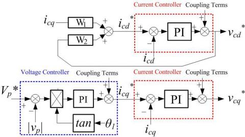
According to Figure 4, the “force-orientation” was realized in this structure using the q-axis through icq*=0, and the PW voltage was modulated by the d-axis. The d-axis current is the amplitude that realize the limit current and ensures the safety of the system.
It is worth noting that the third control structure could achieve the same functions with the simplest structure. Hence, this structure was verified through prototype experiment.
Figure 3. The control structure of CW voltage orientation
Figure 4. The control structure of CW current orientation
The prototype experiment was carried out on a 64kW BDFIG test bench. The input torque was provided by connecting the prototype generator with a frequency-conversion variable-speed motor, which has a MM430 (Siemens) variable frequency drive. The PW was taken as the power supply of 400V/50Hz, and connected to the load, i.e. an induction motor. Meanwhile, the CW was supplied with a self-made bidirectional variable-voltage variable-frequency converter. The speed signal was captured by the generator measurement system (Omron). The system has a resolution of 1,024 cycles/r and consists of three parts: voltage (PW, CW), current (PW, CW) and rotate speed.
The experiment focuses the dynamic performance under load mutation, the impact load and the switch from standalone mode to grid-tied mode.
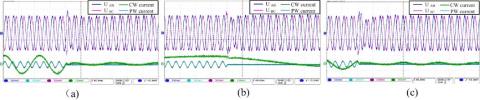
A. The load mutation. Figure 6 shows the dynamic performance from full-load to no-load (80KVA, PF=0.8, lagging). As shown in the figure, the PW voltage surged up to about 100V (the maximum), but it recovered fast within half line-cycle; the control system was always stable because the reference speed ωc was immune to the PW voltage drop.
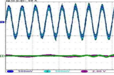
B. The impact load. Figure 7 shows the dynamic performance under impact load (hard-start of a 15kW induction motor). It is clear that the system was still stable, and the PW voltage was recovered within several cycles. During the recovery period, the CW current was easily limited at the given value of 200A, which ensures the safety of the converter system.
C. The switch from standalone mode to grid-tied mode. The mode switch is realized through the following steps. Initially, the load was on the grid, and the BDFIG was load-free. With the switch action, the BDFIG started to be tied to the grid. Then, the grid was cut off, and the load was transferred to the BDFIG. The waveforms are shown in Figure 7.
Figure 5. Dynamic waveforms in (a) 400rpm, (b) 500rpm and (c) 600rpm
Figure 6. Impact load waveforms in (a) 400rpm, (b) 500rpm and (c) 600rpm
Figure 7. The switch from standalone mode to grid-tied mode
This paper presents the CW synchronous speed frame model of BDFIG for power system and establishes the control modes of three orientations methods. Through comparison, it is concluded that the CW-current-oriented model is the simplest one and the physical quantity of orientation (CW current) is easy to control and measure. The control system using voltage and current dual closed-loops can achieve the PW voltage control goals and realize the current limitation. The BDFIG models were proved valid through the prototype experiment.
This work is supported by the Natural Science Foundation of China No.51467018 and High-level Personnel Launch Scientific Research Project of Shihezi University (RCZX201414).
Chen X., Wang X. F., Xiong F. (2013). Research on excitation control for stand-alone wound rotor brushless doubly-fed generator system. International Conference on Electrical Machines and Systems. https://doi.org/10.1109/ICEMS.2013.6754497
Jiang Z. S., Wang S., Ru X. P. (2014). Simulation study of vector control strategy for stand-alone BDFG system. Micromotor, Vol. 47, No. 2, pp. 48-51.
Liu C., Xu D., Zhang X. (2011). Dynamic performance of brushless doubly-fed induction generator during symmetrical grid fault. International Conference on Power Electronics-ECCE Asia, pp. 416-420.
Long T., Shao S. Y., Abdi E., McMahon R., Liu S. (2013). Asymmetrical low-voltage ride through of brushless doubly fed induction generators for the wind power generation. IEEE Trancactions on Energy Conversion, Vol. 28, No. 3, pp. 156-162. https://doi.org/10.1109/TEC.2013.2261818
McMahon R. A., Roberts P. C., Wang X., Tavner P. J. (2006). Performance of BDFM as generator and motor. IEE Proceedings-Electric Power Applications, Vol. 153, No. 2, pp. 289-299. https://doi.org/10.1049/ip-epa:20050289
Poza J., Oyarbide E., Roye D., Rodriguez M. (2006). Unified reference frame DQ model of the brushless doubly fed machine. IEE Proceedings-Electric Power Applications, Vol. 153, No. 5, pp. 726-734. https://doi.org/10.1049/ip-epa:20050404
Poza J., Oyarbide E., Sarasola I., Rodriguez M. (2009). Vector control design and experimental evaluation for the brushless doubly fed machine. IET Electric Power Applications, Vol. 3, No. 4, pp. 247-256. https://doi.org/10.1049/iet-epa.2008.0090
Prousalidis J., Hatzilau I. K., Michaloppulos P., Pavlou I., Muthumuni D. (2005). Studying ship electric energy systems with shaft generator. IEEE Electric Ship Technologies Symposium, pp. 156-162. https://doi.org/10.1109/ESTS.2005.1524669
Shao S. Y., Abdi E., Barati F., Mcmahon R. (2009). Stator-flux-oriented vector control for brushless doubly fed induction generator. IEEE Transaction on Industrial Electronics, Vol. 56, No. 10, pp. 4220-4228. https://doi.org/10.1109/TIE.2009.2024660
Willianson S., Ferreira A. C., Wallace A. K. (2002). Generalised theory of brushless doubly-fed machine. I. Analysis. IEE Proceedings-Electric Power Applications, Vol. 144, No. 2, pp. 111-122. https://doi.org/10.1049/ip-epa:19971051
Xiong F., Wang X. F. (2011). Design and performance analysis of a brushless doubly-fed machine for stand-alone ship shaft generator systems. International Conference on Electrical and Control Engineering, pp. 2114-2117. https://doi.org/10.1109/ICECENG.2011.6057462
Zhang A. L., Jia W. X., Zhou Z. Q., Wang X. (2011). A study on indirect stator-quantities control strategy for brushless doubly-fed induction machine. International Conference on Electrical Machines and Systems, Vol. 32, No. 4, pp. 1-6. https://doi.org/10.1109/ICEMS.2011.6073861