Aicha Benyahia*![]() | Redha Bendoumia
| Redha Bendoumia![]() | Islam Hassani
| Islam Hassani![]()
© 2025 The authors. This article is published by IIETA and is licensed under the CC BY 4.0 license (http://creativecommons.org/licenses/by/4.0/).
OPEN ACCESS
This paper introduces an advanced two-sensor acoustic noise reduction technique, termed DL-VSS-FNLMS, which integrates a deep learning-based variable step-size (DL-VSS) estimation approach into a feed-forward normalized least mean square (FNLMS) adaptive filtering framework. Conventional feed-forward algorithms with a fixed step-size often face limitations when applied to sparse and dispersive acoustic impulse responses, struggling with the trade-off between fast convergence and low steady-state error. To overcome this challenge, we propose a hybrid framework in which a deep neural network is trained on a wide range of acoustic noise signals to estimate optimal step-size parameters. The proposed model leverages combined features extracted from the instantaneous power of the observed noisy speech signal, including Mel-Frequency Cepstral Coefficients (MFCCs) and Gammatone Cepstral Coefficients (GTCCs). This model dynamically guides the selection of the step-size using three Long Short-Term Memory (LSTM) layers, thereby adapting more effectively to varying noise environments. We justify the feature design with a grouped ablation and adopt a minimal configuration (frame energy+MFCC/Δ+GTCC/Δ) that matches the full feature set at moderate SNRs, reserving ERB/Bark/Mel bands only for very low SNR. This integration enables the algorithm to achieve faster convergence and superior speech enhancement. Extensive experiments were conducted to evaluate the proposed method's performance using objective criteria, including mean square error, mean absolute error, correlation coefficient, system mismatch, output segmental signal-to-noise ratio, and cepstral distance. The results demonstrate significant improvements in variable step-size estimation, validating the robustness and efficiency of the deep learning-guided approach.
two-sensor adaptive filtering, LSTM layer, deep learning variable step-size estimation, impulse response identification, adaptive feed-forward structure
Acoustic noise remains a critical challenge in modern telecommunication systems such as hands-free telephony, teleconferencing systems, and hearing aids. Effective noise reduction in these applications requires accurate modeling and adaptive estimation of the acoustic channel. While single-channel noise reduction techniques have shown reasonable performance due to their simplicity and ease of deployment [1], they are often inadequate in environments with highly non-stationary noise or complex acoustic reverberations. Classical approaches such as minimum mean square error (MMSE) estimators [2], spectral subtraction [3], and Wiener filters [4] have been widely adopted but still face trade-offs between noise suppression and speech distortion. To overcome these limitations, adaptive filtering algorithms have been extensively studied in both fullband [5] and subband [6] forms based on adaptive filtering algorithms [5-9]. Nonetheless, single-channel approaches often struggle with non-stationary signals due to the difficulty in robustly estimating the noise characteristics.
Multi-channel techniques, particularly blind source separation (BSS) approaches [10-12], have emerged as powerful alternatives for acoustic noise reduction, leveraging spatial diversity to improve speech intelligibility and signal quality. However, systems with more than two microphones are often impractical for mobile or embedded applications due to increased hardware and computational complexity. As a compromise, two-channel BSS systems offer a balanced trade-off between performance and implementation complexity, and they have demonstrated superior results in terms of speech enhancement and convergence rate [13-15].
In this context, various two-channel feed-forward and backward BSS structures have been proposed, with the feed-forward structure offering better noise suppression but introducing some signal distortion, and the backward structure providing cleaner output signals at the cost of lower noise reduction. To mitigate these issues, post-filtering techniques and symmetric adaptive decorrelation (SAD) algorithms have been introduced [16, 17]. Furthermore, several adaptive filtering algorithms tailored to two-channel BSS in sub-band form have been proposed to further improve convergence behavior and robustness in reverberant environments [16, 18, 19]. More recently, two-channel variable step-size (VSS) NLMS algorithms have been developed to address the long-standing trade-off between fast convergence and low steady-state misadjustment [20]. A forward-and-backward two-channel VSS NLMS framework was introduced, where step-size adaptation was guided by a signal decorrelation function [15]. However, these conventional VSS methods still exhibit suboptimal performance in sparse acoustic environments, especially under complex noise conditions.
To address these limitations, in this paper, we propose a novel deep learning-based variable step-size estimation mechanism implemented on two-sensor noise reduction technique based on NLMS adaptive filtering. A deep neural network is trained on multiple types of acoustic noise signals to learn the relationship between noisy-signal power characteristics and optimal step-size values. Our novelty is an MSD-supervised, VAD-gated step-size and its integration in a two-sensor FF-NLMS system, with policy-aligned features computed on only noisy frames. This adaptive mechanism enables the algorithm to dynamically adjust the step-size parameters, resulting in faster convergence and improved speech quality in sparse and dispersive impulse response situations. The proposed method is rigorously evaluated through extensive experiments using objective performance criteria. Experimental results confirm the effectiveness and robustness of the deep learning-guided approach for variable step-size estimation and two-sensor acoustic noise reduction.
This paper is presented as follows: in Section 2, the two-channel convolutive mixing problem between speech and noise signals is detailed. Section 3 is reserved for the presentation of the proposed two-sensor Feed-forward technique adapted by new deep learning-based variable step-size mechanism. The comparative simulation results are presented in Section 5, and finally, the conclusion of this paper is presented in Section 6.
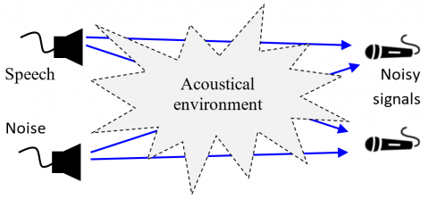
In many real-world acoustic environments, such as hands-free telephony or conference systems, speech signals captured by microphones are not direct but rather mixed versions due to propagation effects and reverberations. These captured signals result from a convolutive mixing process between multiple sources and microphones [21, 22]. Specifically, the two-channel convolutive mixing system considers the case of two sources, speech and noise, and two sensors (see Figure 1).
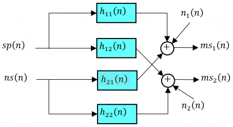
As shown in Figure 2, the speech signal $s p(n)$ and the noise signal $ns(n)$ propagate through an acoustic environment before being captured by the microphones [21]. Each propagation path is characterized by an impulse response that models the effect of the room acoustics, source-to-microphone distance, and reflection patterns.
Figure 1. General presentation of the two-channel acoustical convolutive system
Figure 2. Full Model of the two-channel acoustical convolutive system [11, 12, 14, 15]
The two noisy $m s_1(n)$ and $m s_2(n)$, captured at the microphones, can be mathematically modeled as:
$\begin{gathered}m s_1(n)=s p(n) * h_{11}(n)+n_1(n)+n s(n) * h_{21}(n)\end{gathered}$ (1)
$\begin{aligned} m s_2(n)=n s(n) & * h_{22}(n)+n_2(n)+s p(n) * h_{12}(n)\end{aligned}$ (2)
where,
$h_{11}(n)$ and $h_{22}(n)$ are the direct paths from the speech and noise sources to their nearest microphones,
$h_{12}(n)$ and $h_{21}(n)$ represent the cross-paths between sources and distant microphones,
$n_1(n)$ and $n_2(n)$ are additive noises (e.g., sensor noise or background interferences),
" * " denotes the linear convolution operator.
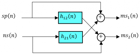
In practical acoustic signal processing scenarios, especially for real-time noise reduction applications, it is often beneficial to adopt a simplified model of the two-channel convolutive mixing system presented in Figure 3 [11, 12].
Figure 3. Simplified Model of the two-channel acoustical convolutive system [14, 15]
The cross-path filters $h_{12}(n)$ and $h_{21}(n)$ still model the propagation of signals from the remote source to the non-adjacent microphone and are kept general (non-trivial) [11, 12, 14, 15]. Using these simplifications, the observed signals at the microphones become:
$m s_1(n)=s p(n)+n s(n) * h_{21}(n)$ (3)
$m s_2(n)=n s(n)+s p(n) * h_{12}(n)$ (4)
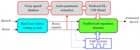
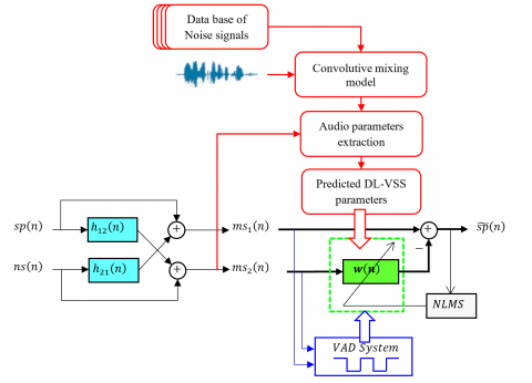
In this sub-section, we present the proposed two-sensor feed-forward structure based on deep learning variable step-sizes approach and we give the optimal solutions of adaptive filters, as we present the formulations of the DL-VSS-FNLMS algorithm in the time-domain implemented on this structure. The global model of the proposed two-sensor Feed-forward algorithm is presented in Figure 4.
Figure 4. Global structure of proposed DL-VSS-FNLMS
Figure 5. Detailed presentation of proposed DL-VSS-FNLMS algorithm
Noting that, all two-sensor Feed-forward techniques are based on the assumptions that the sources signals $sp(n)$ and $ns(n)$ are mutually independent, i.e., $E[s p(n) n s(n-m)]=0, \forall m$, or alternatively, this implies that they are uncorrelated. The proposed DL-VSS-FNLMS algorithm introduces a deep learning-assisted variable step-size adaptive filtering framework for acoustic noise reduction, a database of noise signals is first combined with clean speech through a convolutive mixing model to simulate real-world noisy environments. A deep learning model predicts the optimal adaptation parameters for the adaptive filter $w(n)$. The proposed algorithm integrates a voice activity detector (VAD), which identifies speech-active and noise-only segments to control the filter adaptation. This selective update mechanism enhances noise suppression during active speech and reduces computational overhead during silent or noise-only periods, resulting in more efficient and targeted filter adaptation. The detailed structure of proposed DL-VSS-FNLMS algorithm is presented in Figure 5.
3.1 Voice activity detection mechanism
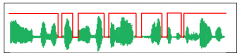
The proposed DL-VSS-FNLMS algorithm incorporates a voice activity detection (VAD) mechanism to guide the adaptation of its filtering process. VAD systems are commonly used to distinguish between segments of speech that contain only background noise or silence, as presented in Figure 6. This information is then used to control how and when filter coefficients are updated.
In the DL-VSS approach, adaptive filter w(n) processes the incoming noisy signal. A key feature of this method is that the filter w(n) is updated only during noise-only intervals or inactive speech periods. This selective adaptation strategy reduces the computational load and improves overall efficiency. Figure 7 shows a schematic of the VAD system, detailing how it manages the filter updates within the two-sensor Feed-forward configuration of the DL-VSS algorithm.
Figure 6. Example of speech signal segmentation using VAD
Figure 7. The control of adaptive filter by VAD system
To enhance the adaptability of the proposed two-sensor Feed-forward algorithm, the step-size parameter $\mu_{D L}(n)$ is dynamically estimated using a deep learning model. These parameters are crucial for ensuring both convergence and efficient tracking performance of the adaptive filter $\boldsymbol{w}(n)$. The prediction of the variable step-size is achieved by training a neural network using relevant input features derived from the noisy speech signal during noise periods, as identified by the VAD system.
3.2 Adaptive filter formulation
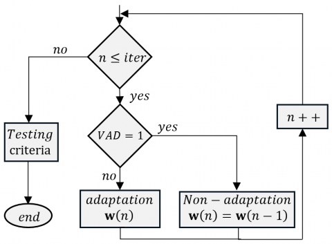
For updating the adaptive filter $\boldsymbol{w}(n)$, we propose to use two-sensor Feed-forward structure adapted by the NLMS algorithm but controlled in this case by the new deep learning variable step-sizes parameters. The update formula of adaptive filter by this new algorithm are adjusted according the VAD given as follows:
$\boldsymbol{w}(n)=\left\{\begin{array}{cl}\boldsymbol{w}(n-1)+\mu_{D L}(n) \frac{\widetilde{s p}(n) \boldsymbol{m} \boldsymbol{s}_2(n)}{\varepsilon+\left\|\boldsymbol{m} \boldsymbol{s}_2(n)\right\|^2} & \text { if } V A D=0 \\ \boldsymbol{w}(n-1) & \text { if } V A D=1\end{array}\right.$ (5)
where, $\mu_{D L}(n)$ represents the adaptive step-size estimated by deep learning model, with the necessary and sufficient condition to guarantee the convergence and the stability of this algorithm in the MSE sense is $0<\mu_{D L}(n)<2$, and $\varepsilon$ presents a very small positive constant. The tap-weight vectors of the adaptive filters $\boldsymbol{w}(n)$ is defined respectively by:
$\boldsymbol{w}(n)=\left[w_1(n), w_2(n), \ldots, w_M(n)\right]^T$
We also define vector (last M values) of inputs noisy signal, $m s_2(n)$ as:
$\boldsymbol{m} \boldsymbol{s}_2(n)=\left[m s_2(n), m s_2(n-1), \ldots, m s_2(n-M+1)\right]^T$
where, M is the length of adaptive filter.
3.3 Proposed minimization of variable step-size
The adaptation step-size is a key parameter in the performance of adaptive filter $w(n)$. To ensure rapid convergence and accurate tracking of the optimal filter coefficients, we define the step-size as the result of a minimization process that targets the mean-square deviation (MSD) between the ideal impulse response and the current filter weights. We aim to find the optimal step-size parameter $\mu_{D L}^{o p t}(n)$ for adaptive filter $w(n)$ such that the deviation from the ideal filter $h_{21}$ is minimized:
$\xi(n)=\boldsymbol{h}_{21}-\boldsymbol{w}(n)$ (6)
We define the expressions of MSD for adaptive filter $\boldsymbol{w}(n)$ as follows:
$M S D(n)=E\left[\|\xi(n)\|^2\right]$ (7)
We derive a relation showing how MSD evolves over time as a function of the step-size parameter. After deriving from the previous equation and computing the squared Euclidean model, we arrive at the following equation:
$\begin{aligned} \operatorname{MSD}(n)-\operatorname{MSD} & (n-1) =\mu_{D L}^2 E\left[\frac{(\widetilde{s p}(n))^2}{\sigma_2(n)}\right] -2 \mu_{D L} E\left[\frac{\xi^T(n-1) \widetilde{\mathbf{m s}}_{\mathbf{2}}(n) \widetilde{s p}(n)}{\sigma_2(n)}\right]\end{aligned}$ (8)
To ensure improvement, $\operatorname{MSD}(n)-\operatorname{MSD}(n-1)<0$, given that $\mu_{D L}^{\text {opt }}(n)<2\, \nabla(n)$. Here, $\nabla(n)$ is small value calculated from the cross-correlation between the input and output signal of adaptive filter. To avoid direct computation of expectations, we propose the recursive formulas, $\mu_{D L}^{o p t}(n)= \mu_{\max } \widetilde{\nabla}(n)$, with the estimated quantities $\widetilde{\nabla}(n)$ is given by,
$\widetilde{\nabla}(n)=\mu_{\max }\left[\frac{\|\mathbf{Q}(n)\|^2}{\rho+\|\mathbf{Q}(d)\|^2}\right]$ (9)
where, $\mathbf{Q}(n)$ captures the cross-correlation dynamics and is updated over time, using the next recursive estimation,
$\mathbf{Q}(n)=\lambda \mathbf{Q}(n-1)+\frac{(1-\lambda)}{\sigma_2(n)+\varepsilon} \widetilde{s p}(n) \widetilde{\mathbf{m s}}_2(n)$ (10)
with $0<\lambda_i<1$. This theoretical optimal value $\mu_{D L}^{\text {opt }}(n)$ is then used as the training target for a deep neural network. The network learns to predict the step-size dynamically from combined features, replicating this minimization behavior without needing explicit MSD calculations during inference.
3.4 Deep learning VSS parameters estimation
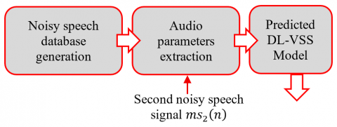
To enable effective prediction of the variable step-size parameter $\mu_{D L}(n)$ in the two-sensor adaptive Feed-forward NLMS process, it is important to provide the deep learning model with input features that accurately reflect the dynamic properties of the second noisy speech signal $m s_2(n)$. This section outlines the feature extraction methodology used to construct informative input vectors for training the neural network. This part is divided in three important parts, (i) noisy speech database, (ii) audio parameters extraction, and (iii) variable step-sizes deep learning prediction, as presented in Figure 8.
Figure 8. Three parts of deep learning VSS parameters extraction
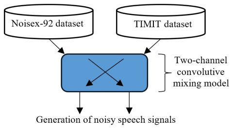
3.4.1 Noisy speech database generation
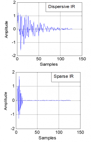
In this part, the convolutive mixing model used in this work simulates the real-world interaction between a speech source and its acoustic environment. It is characterized by two types of acoustic impulse responses, dispersive and sparse [23-25], which reflect the physical behavior of sound propagation in closed spaces. The dispersive impulse responses are characterized by long-duration, densely populated coefficients that model environments with rich reverberation and multiple reflections, such as large rooms or halls, where the energy spreads over time. In contrast, the sparse impulse responses contain only a few significant nonzero coefficients, representing environments with limited reflections or directional propagation paths, such as small or acoustically treated spaces. This realistic modeling is essential for generating training data that challenges the adaptive filtering system and allows the deep learning model to learn context-aware step-size adaptation strategies. To train and evaluate the deep learning model for variable step-size prediction in adaptive filtering, we constructed a dataset of noisy speech signals composed of clean speech signals combined with various environmental noises using a two-channel convolutive mixing model. The clean speech signals were taken from publicly available speech corpora, i.e., TIMIT [26], which provide high-quality recordings from multiple speakers under clean conditions. These signals serve as the primary content to be enhanced by the adaptive filtering process.
After preparing the clean speech recordings, we mixed them with several different noise types selected from the NOISEX-92 database [27]. These included a variety of real-world acoustic environments such as white noise, babble noise, F16 aircraft noise, factory1 noise, HF channel noise, and buccaneer noise. These diverse noise environments were chosen to evaluate the robustness and generalization capability of the proposed algorithm under both stationary and non-stationary interference. Each noise signal was convolved with the clean speech using a two-channel convolutive mixing model, which simulates the propagation of noise through an acoustic environment such as a room or enclosure. This model allows the creation of realistic mixed signals that closely replicate the challenging conditions encountered in practical applications.
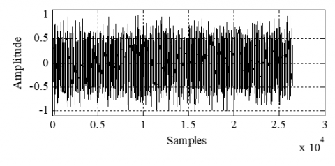
The resulting dataset includes a wide variety of speech-in-noise examples that reflect both temporal and spectral variability (see Figure 9). These mixtures are essential for training the neural network to predict step-size parameters that respond appropriately to dynamic and nonstationary acoustic environments.
Figure 9. Generation of noisy speech database
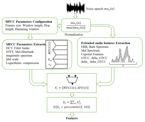
3.4.2 Audio parameters extraction
The procedure begins with signal normalization to reduce amplitude variability, followed by the extraction of Mel-Frequency Cepstral Coefficients (MFCCs), which are commonly used in speech and audio analysis for their ability to capture phonetic and spectral content. To complement these, additional perceptual and cepstral features, including Gammatone Cepstral Coefficients (GTCCs), their first and second temporal derivatives, and energy-based spectral descriptors from the ERB, Bark, and Mel scales, are computed using the audio Feature Extractor. All extracted features are then concatenated into unified vectors representing each time frame of the speech signal. To further refine the training data and improve the model’s ability to distinguish between active and inactive speech regions, a silence detection step based on frame energy is applied. The resulting feature set provides a rich and discriminative representation of the acoustic signal.
(i) Second noisy speech signal preprocessing
The second input noisy speech signal $m s_2(n)$ of the twosensor Feed-forward structure, is first normalized to ensure that its amplitude remains within the range $[-1,1]$. The normalization was performed using the following operation:
$m s_{2, n}(n)=\frac{m s_2(n)}{\max \left|m s_2(n)\right|}$ (11)
Its main objective of the noisy speech normalization is to improve numerical stability during signal processing by scaling the signal amplitude within a predictable range, thus preventing computational errors or loss of precision. Additionally, it helps maintain the quality and comparability of extracted features, making them less sensitive to variations in recording volume. This ensures that the deep learning model can generalize more effectively across different speech recordings, regardless of their original amplitude levels.
(ii) MFCC coefficient configuration
The MFCCs are widely used acoustic features in speech and audio processing due to their ability to compactly represent the short-term power spectrum of a signal in a perceptually meaningful way. In this work, MFCCs were extracted as part of the input features for the deep learning model, following a carefully designed segmentation and preprocessing procedure. Given that speech is a non-stationary signal, it must be analyzed over short segments where it can be approximated as quasi-stationary. To achieve this, the signal was divided into overlapping frames using the three important parameters:
Window length: A duration of 25 milliseconds was selected, corresponding to $L_W=\operatorname{round}\left(0.025 \times \mathrm{f}_s\right)$, where fs is the sampling rate. This window size strikes a balance between temporal resolution (to capture rapid transitions such as phonemes) and frequency resolution (to preserve spectral content).
Hop length (overlap): A shift of 10 milliseconds was applied between successive frames: $L_H=\operatorname{round}\left(0.01 \times \mathrm{f}_s\right)$ resulting in a frame overlap of 15ms. This overlap ensures continuity across frames, reduces the risk of missing transient information, and provides smoother transitions in the extracted features.
$L_{\text {overlap }}=L_W-L_H$ (12)
Hamming window: To minimize spectral leakage due to discontinuities at the frame boundaries, a Hamming window was applied to each frame. This window gradually attenuates the signal at the edges of each segment, improving the accuracy and robustness of the spectral analysis.
$\begin{gathered}H w(n)=0.54-0.46 \times \cos \left(\frac{2 \pi n}{L_W-1}\right), \\ 0 \leq n<L_W\end{gathered}$ (13)
(iii) MFCC coefficient extraction
Once the signal was windowed and preprocessed, 13 MFCCs were computed per frame. The process follows these main steps: Short-Time Fourier Transform (STFT) to convert each frame into the frequency domain, Mel-filterbank processing, where the magnitude spectrum is passed through a series of triangular filters spaced according to the Mel scale to mimic human auditory perception, Logarithmic compression to emulate the non-linear perception of loudness, and finally the Discrete Cosine Transform (DCT) to decorrelate the filterbank outputs and retain only the most relevant coefficients.
The extraction of MFCCs is based on a series of mathematical transformations applied to audio signal segments, aiming to capture relevant spectral characteristics for acoustic analysis. The mathematical formulation is given by:
$\operatorname{MFCC}(t)=\operatorname{DCT}\left(\log \left(\operatorname{MelSpectrum}\left(m x_{2, n}(t)\right)\right)\right.$ (14)
where, $m x_{2, n}(t)$ is the time-domain signal segment centered at time n , MelSpectrum represents the application of a triangular filterbank based on the Mel scale to the signal's spectrum, $\log$ simulates the nonlinear human perception of loudness, and $D C T$ is used to decorrelate the $\log _{-} M e l$ features and compact the information.
The output of the Mel_filterbank Energy is defined by:
$E_m=\log \left(\sum_k\left|M X_{2, n}[k]\right|^2 \times H_m[k]\right)$ (15)
with, $M X_{2, n}[k]$ is the FFT of the windowed noisy signal $m x_{2, n}(n), H_m[k]$ presents Mel filterbank, $\left|M X_{2, n}[k]\right|^2$ the power spectral density of the noisy signal $m x_{2, n}(n)$, and finally the Logarithm is applied to match human auditory perception. Then, the cepstral coefficients $c_n$ are computed as,
$\begin{gathered}c_n=\sum_{m=1}^M E_m \times \cos \left(n \times \frac{\pi}{M} \times\left(m-\frac{1}{2}\right)\right), 0 \leq n <N_{\text {coeffs }}\end{gathered}$ (16)
$M$ is the number of Mel filters, $N_{\text {coeffs }}$ is the number of desired cepstral coefficients (typically 12 or 13), and it converts the M_logMel energies into $N_{\text {coeffs }}$ decorrelated cepstral coefficients.
(iv) Extended spectral feature extraction
In addition to the standard MFCCs, a broader and more perceptually-informed set of audio features was extracted. This step aims to capture complementary spectral characteristics that enhance the robustness and expressiveness of the features fed into the deep learning model, particularly in the presence of noise. The following spectral representations were computed, each based on different psychoacoustic models of human hearing:
Equivalent Rectangular Bandwidth Spectrum (ERB): This feature emulates the frequency resolution of the human cochlea by analyzing the signal across perceptually equivalent frequency bands. It provides a fine-grained spectral decomposition aligned with auditory filter bandwidths.
Given a short-time Fourier-transformed magnitude spectrum $\left|M X_{2, n}(f)\right|^2$, the ERB Spectrum at frame n is computed by filtering this spectrum through a bank of ERBspaced filters $H_m^{E R B}(f)$:
$E R B_m(n)=\log \left(\sum_f\left|M X_{2, n}(f)\right|^2 \times H_m^{E R B}(f)\right)$ (17)
with $M X_{2, n}(f)$ is the Fourier transform of the signal frame centered at time $\mathrm{t}, H_m^{E R B}(f)$ is the frequency response of the $m^{\text {th }}$ Gammatone filter in the ERB-scaled filterbank, $m= 1,2, \ldots, M$ where $M$ is the number of ERB bands.
Bark Spectrum: This representation divides the frequency axis into critical bands that reflect how the human ear groups frequencies. It is especially useful in capturing perceptually relevant changes in the spectral envelope.
Mel Spectrum: The Mel scale approximates how humans perceive pitch. It is linear in the low-frequency range and logarithmic in the high-frequency range, thereby giving more resolution to lower frequencies where speech energy is concentrated.
These spectral features provide multidimensional insights into the energy distribution across the perceptual frequency space, helping the neural model better interpret phonetic and prosodic content.
Cepstral Features: GTCC and Derivatives
GTCC: Similar to MFCCs but derived from a Gammatone filterbank, which is believed to more accurately model the frequency selectivity of the human auditory system. GTCCs are particularly effective in noisy environments and provide an alternative spectral representation of the audio signal.
Steps for GTCC extraction
Let $m x_{2, n}(n)$ be a time-domain frame centered at time t, and apply the windowed STFT:
$M X_{2, n}(k)=\operatorname{SFTT}\left(m x_{2, n}(n)\right)$ (18)
Power Spectrum
$P_t(k)=\left|M X_{2, n}(k)\right|^2$ (19)
Apply a Gammatone filterbank $G_m[k]$ (with $M$ filters):
$E_m(t)=\sum_k P_t(k) \times G_m[k]$ (20)
Logarithmic Compression
$\widetilde{E}_m(t)=\log \left(E_m(t)+\varepsilon\right)$ (21)
with $\varepsilon$ is a small constant to avoid $\log (0)$
Discrete Cosine Transform (DCT)
$\operatorname{GTCC}_n(t)=\sum_{m=1}^M \tilde{E}_m(t) \times \cos \left(\frac{n \pi}{M} \times\left(m-\frac{1}{2}\right)\right), 0 \leq n<N_{\text {coeffs }}$ (22)
Delta Coefficients ($\Delta G T C C$) and Delta-Delta Coefficients $\left(\Delta^2 G T C C\right)$: These temporal derivatives of GTCCs represent the first and second-order changes over time analogous to velocity and acceleration. By capturing how spectral features evolve, they add important dynamic context that is essential for modeling time-varying signals like speech.
$\Delta G T C C$ represent the first-order temporal derivatives (rate of change):
$\Delta G T C C_n(t)=\frac{\sum_{l=0}^L l \times\left(G T C C_n(t+l)-G T C C_n(t-l)\right)}{2 \times \sum_{l=0}^L l^2}$ (23)
where, L is the window size for derivative calculation (usually 2).
$\Delta^2$GTCC is the second-order temporal derivatives (acceleration):
$\begin{aligned}\Delta^2 \operatorname{GTCC}_n(t) =\frac{\sum_{l=0}^L l \times\left(\Delta G T C C_n(t+l)-\Delta G T C C_n(t-l)\right)}{2 \times \sum_{l=0}^L l^2}\end{aligned}$ (24)
The final extended spectral feature vector for each time frame t is defined as:
$\operatorname{AFE}(t)=\left[\begin{array}{c}G T C C_n(t), \Delta G T C C_n(t), \Delta^2 G T C C_n(t), \\ \operatorname{Mel}(t), \operatorname{Bark}(t), E B R(t)\end{array}\right]$ (25)
This rich, multidimensional representation significantly enhances the descriptive power of the input features, enabling the neural network to more accurately model and adapt to complex acoustic environments.
(v) Features combination
Once the spectral and cepstral features—including MFCCs, spectral representations (Mel, Bark, ERB), and GTCCs with their temporal derivatives—have been extracted, they are concatenated to form a single combined feature matrix. This process brings together complementary aspects of the speech signal, enriching the representation for downstream learning tasks.
By merging features with different perceptual and spectral perspectives, the combined matrix captures both the static and dynamic properties of the speech content. This multidimensional feature set serves as a robust and informative input to the deep learning model, enabling it to better distinguish between speech and noise, and to adapt effectively in complex acoustic environments.
$F_t=[M F C C(t), A F E(t)]$ (26)
The feature set is chosen to support step-size control rather than phonetic recognition. Frame energy stabilizes $\mu_{D L}(n)$ during bursts; MFCC/$\Delta$ capture near-end speech leakage that risks speech distortion if the step size is too large; GTCC/$\Delta$ are more noise-robust and track narrowband/colored interferers; ERB/Bark/Mel provide coarse, low-variance spectral envelopes that help at very low SNR.
(vi) Automatic silence detection
To enhance the training dataset for the step-size prediction model, Automatic silence detection was applied. Frame-level energy was computed as the squared norm of each feature vector:
$E_t=\sum_{i=1}^D F_{t, i}^2$ (27)
where, $D$ is the dimension of the feature vector. A threshold based on the $10^{{th }}$ percentile of the energy distribution was used to identify silent frames:
$Silence\quad Frames =\left\{t \mid E_t<\right.$ percentile $\left.(E, 10)\right\}$ (28)
These silent frames are particularly informative, as they typically correspond to regions where the optimal adaptation step-size should be small or even zero. This enables the neural model to better generalize across both speech-active and inactive segments.
(vii) Steps of audio features extraction
In Figure 10, we present all steps used for audio feature extraction based on all subparts presented previously.
Figure 10. Proposed audio features extraction for proposed deep learning model
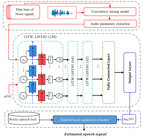
3.5 Deep learning model for variable step size estimation
This study introduces a deep learning-based model designed to estimate the adaptive step-size parameters, specifically $\mu_{D L}(n)$, for the dual-microphone NLMS algorithm. The model's objective is to dynamically predict this parameter directly from acoustic features extracted from noisy speech. The chosen architecture is a Recurrent Neural Network (RNN) employing stacked Long Short-Term Memory (LSTM) layers, which are particularly effective at capturing temporal dependencies inherent in sequential audio features.
(1) Data Preparation and Normalization
The input Features presented previously in subsection 3.4. The network's input is a comprehensive feature matrix derived from preceding stages, integrating MFCCs, GTCCs, and various other spectral representations (ERB, Bark, Mel). These features are concatenated to form a rich representation for each time frame of the noisy speech signal. The corresponding labels for the network are the step-size parameter $\mu(n)$. These are computed for each time frame using a predefined analytical method presented previously in subsection 3.3. The entire dataset is randomly partitioned into training and testing subsets, maintaining a 70:30 ratio respectively.
To ensure numerical stability and consistency during the training phase, z-score normalization is applied to the input features. This normalization uses the mean and standard deviation calculated exclusively from the training set. This step ensures equal contribution from all feature dimensions during learning and accelerates convergence. The training features are transposed and converted into a sequence format suitable for time-series modeling by the RNN.
(2) Network Architecture
The architecture of the proposed Recurrent Neural Network (RNN), as presented in Figure 11, is specifically designed to model the temporal evolution of acoustic features and to predict the variable step-size parameters of the dual-microphone NLMS algorithm. The network leverages a stack of Long Short-Term Memory (LSTM) layers, which are well-suited for sequence learning due to their ability to capture long-range dependencies.
Figure 11. Detailed deep learning model used for acoustic noise reduction
The architectural components are detailed below:
Input Layer: The model begins with a sequenceInputLayer, which accepts sequential input data. This layer is configured to match the dimensionality of the input feature vector (i.e., the number of concatenated acoustic features per time frame).
First LSTM Block: The first recurrent block consists of an LSTM layer with 128 memory units. This layer processes the temporal sequence and captures short- to medium-term dependencies across frames. A dropout layer with a dropout rate of 20% is applied immediately after this layer to reduce overfitting and improve generalization.
Second LSTM Block: A second LSTM layer with 64 units is stacked atop the first to enable deeper sequence representation learning. This layer further refines the model’s capacity to understand longer-term temporal structures. Again, a 20% dropout is applied post-activation.
Third LSTM Block: The third and final LSTM layer contains 32 units and is configured with OutputMode ='last', ensuring that only the final hidden state is propagated forward. This design choice enables the network to summarize the entire input sequence into a compact latent representation, capturing the most relevant temporal information for the prediction task.
Fully Connected Layers: The compressed temporal representation is passed through two fully connected (dense) layers: (i) The first dense layer has 64 neurons, followed by a ReLU activation function to introduce non-linearity and enable the learning of complex mappings. (ii) the second dense layer comprises a single neuron, responsible for outputting the predicted continuous-valued step-size coefficient for the current frame.
Output Layer: A regression layer is used as the final output component. It maps the scalar output from the dense layer to the real-valued target, allowing the model to perform a frame-level regression task.
(3) Training Strategy
To effectively optimize the proposed RNN architecture for variable step-size prediction, a carefully designed training protocol was adopted. This strategy ensures robust convergence, generalization, and efficient utilization of computational resources. The key components of the training process are described as follows:
Optimization Algorithm: The network parameters are optimized using the Adam optimizer, a widely adopted stochastic gradient-based method that combines the advantages of Adaptive Gradient Algorithm (AdaGrad) and Root Mean Square Propagation (RMSProp). Adam provides efficient and stable convergence through adaptive learning rates and momentum terms for each parameter.
Training Duration: The training process is executed over 100 full epochs, allowing sufficient opportunity for the model to learn complex temporal patterns and minimize prediction error. Empirical tuning confirmed that this duration balances model performance and training time.
Mini-Batch Configuration: A mini-batch size of 32 samples is employed during training. This batch size provides a good trade-off between convergence stability and computational efficiency, especially for time-series data where memory consumption can become a constraint.
Data Shuffling: To enhance the model's ability to generalize beyond the training dataset and prevent overfitting to sequence order, shuffling is applied to the training data at the end of each epoch. This disrupts any spurious correlations due to ordering in the training sequences.
Loss Monitoring and Custom Callbacks: A custom callback function is integrated into the training loop to record and monitor the evolution of the training loss after each epoch. This enables continuous assessment of the learning progress and early detection of issues such as stagnation or overfitting.
Software Implementation: The entire model training pipeline, including network definition, loss tracking, and data preprocessing, is implemented using Deep Learning Toolbox. Specifically, the trainNetwork function is utilized to manage the iterative optimization process.
This RNN-based predictor provides a robust, data-driven mechanism to adaptively determine optimal step-size parameter for the NLMS algorithm, thereby improving its robustness and convergence characteristics across diverse acoustic environments.
3.6 Enhanced speech signal estimation
In this structure, we use an adaptive filter $\boldsymbol{w}(n)$ to identify the two acoustical impulse response $\boldsymbol{h}_{21}$ of two-channel convolutive mixture system. In the last part of proposed algorithm and after convergence, the optimal solution is given by some studies [11, 15, 21, 22]:
$\boldsymbol{w}(n)=\boldsymbol{h}_{21}$ (29)
With this optimal solution of the adaptive filters, the estimated speech signal can be rewritten as follows:
$\begin{aligned} \widetilde{s p}(n)=s n(n) & *\left[\boldsymbol{h}_{21}-\boldsymbol{w}(n)\right]+s p(n) *\left[\delta(n)-\boldsymbol{h}_{12} * \boldsymbol{w}(n)\right]\end{aligned}$ (30)
$\widetilde{s p}(n)=s p(n) * D_s$ (31)
where, $D_s$ represents small distortion.
4.1 Input/Output signals of mixing model
This section provides a detailed simulation analysis to assess the effectiveness of the proposed DL-VSS-FNLMS algorithm in various noisy acoustic environments. The simulation experiments are based on a realistic convolutive mixing model, as illustrated in Figure 3. This model involves the linear convolution of two independent acoustic source signals:
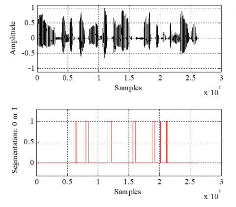
(1) Source 1: A clean, phonetically balanced speech signal from a single speaker, sampled at 8kHz and encoded with 16-bit precision. The temporal waveform and the associated voice activity detection signal for this speech input are displayed in Figure 12. This original speech signal is a French sentence that lasts approximately 4s, measured under actual circumstances using data from the [28] phonetically balanced test/database. The AURORA database is where this speech signal came from [29].
Figure 12. Original speech signal and generated segmentation
(2) Source 2: A point-source noise representing real-world disturbances. We made use of a variety of noise sources, including white, babble, F16 aircraft, factory1, Hfchannel, and buccaneer. It should be noted that all of these noise signals are real, sampled at 8 kHz, and encoded at 16 bit. Figure 13 shows an example illustration of a white noise signal.
The mixture signal, simulating a reverberant and noisy environment, is generated by convolving each source with a distinct room impulse response, as defined by the acoustical mixing model [30]. These impulse responses, shown in Figure 14, characterize the acoustic paths from each source to the microphones in a simulated room [31].
The resulting noisy observations, presented in Figure 15, correspond to an input signal-to-noise ratio (SNR) of -6dB. This simulation framework enables a robust and fair evaluation of the adaptive algorithms under controlled yet realistic conditions, highlighting the benefits of the proposed DL-VSS method in terms of both convergence and perceptual speech quality.
Figure 13. Noise signal
Figure 14. Examples of real dispersive and sparse impulse responses
Figure 15. Two noisy speech signals with Input-SNR=-6dB
4.2 Parameters and testing criteria
In all presented simulations throughout this study, the proposed advanced methods were evaluated using a consistent set of input signals and a range of fixed and adaptive parameters. These parameter values were carefully selected to ensure a fair and comprehensive comparison under various acoustic conditions. These diverse noise types were chosen to simulate realistic and challenging environments for testing noise reduction algorithms. The acoustic propagation was modeled using acoustic impulse responses with identical lengths for both channels (M=128), which simulate reverberant paths between sources and sensors. The noisy observations were generated at different input signal-to-noise ratio (SNR) levels: - 6dB, - 3dB, 0dB, 3dB and +6dB, independently applied to both input channels (SNR1 and SNR2). These varying SNR levels enabled a detailed evaluation of algorithm robustness under low, medium, and high noise scenarios.
For the evaluation of the proposed algorithm, a wide range of internal parameters were tested. The maximum values of the adaptive step sizes, denoted $\mu_{\max }$, were explored using four different values: $0.5,0.9$, and 1.5. The algorithm's performance also depended on several fine-tuned constants, including: $\lambda=0.67, \rho=2$ and $\varepsilon=10^{-6}$. These parameters were crucial in determining the behavior of the adaptive filters, particularly in convergence speed, numerical stability, and noise suppression efficiency. The chosen values reflect a compromise between rapid adaptation and avoidance of instability or overfitting in the presence of strong noise components. These parameters were chosen after several simulation rounds on a held-out validation set via a coarse-tofine search (averaged over multiple seeds) and then frozen before testing.
The proposed algorithm was evaluated in a two-channel convolutive mixing system using two types of impulse responses: dispersive and sparse. The test is based on the following performance metrics:
Combined features and detected silence periods
Time-domain VSS evolution: We examine the temporal evolution of the variable step-size parameters produced by proposed DL model. This qualitative assessment helps to visualize the waveform clarity and transient behavior of the reconstructed speech after noise reduction stage.
Objective criteria for DL model: In this part, we propose to evaluate the performance of the deep learning model by using three criteria: the Mean Square Error (MSE), Mean Absolute Error (MAE), and the Correlation Coefficient (R2).
System mismatch (SM): The SM is calculated as the average of the differences between the real impulse response coefficients $\mathbf{h}_{21}$ and the obtained adaptive filter coefficients $\mathbf{w}$. This criterion serves as a key indicator of the convergence speed and stability of the adaptive filtering process.
$\left[S M_n\right]_{d B}=20 \log _{10}\left[\frac{\left\|\mathbf{h}_{21}-\mathbf{w}\right\|}{\left\|\mathbf{h}_{21}\right\|}\right]$ (32)
The SM is computed across segments of 128 samples.
Segmental Signal-to-Noise Ratio (Seg-SNR): The Seg-SNR quantifies the improvement in signal quality after enhancement, particularly in terms of noise suppression.
$\begin{gathered}{\left[\operatorname{Seg} \operatorname{SNR} R_n\right]_{d B}} =10 \log _{10}\left[\frac{\sum_{i=1}^N|\operatorname{sp}(i)|^2}{\sum_{i=1}^N|\operatorname{sp}(i)-\widetilde{\operatorname{sp}}(i)|^2}\right] \text { if } \operatorname{VAD}(i) =1\end{gathered}$ (33)
It is defined as the signal-to-noise ratio computed over short, fixed-length segments (each containing 512 samples), enabling a localized analysis of enhancement performance. Higher Seg-SNR values correspond to better noise attenuation and speech preservation.
Cepstral distance (CD): To estimate the distortion of the enhanced speech, we used the CD criterion. The CD quantifies the log-spectrum distance between the original speech and enhanced ones. It is a robust measure that correlates well with the perceived quality of speech,
$[C D]_{d B}=\sum_{i=1}^N I S F T[\log (|S P(\omega, i)|)-|\widetilde{S P}(\omega, i)|]^2$ (34)
where, $I S F T[$.$]$ denote the inverse-short-Fourier-transform, $S P(\omega, i)$ and $\widetilde{S P}(\omega, i)$ are the short-Fourier-transform (SFT) of the original speech $s p(\omega, i)$ and the enhanced $\widetilde{s p}(\omega, i)$.
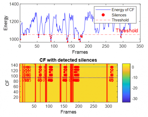
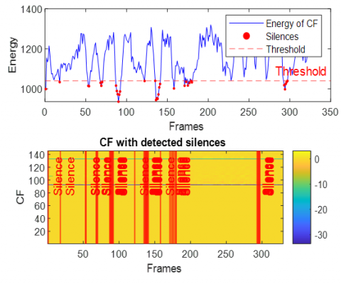
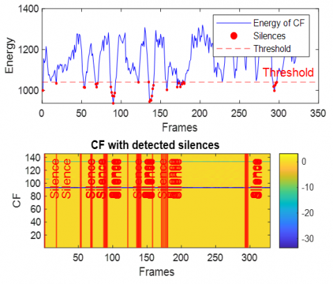
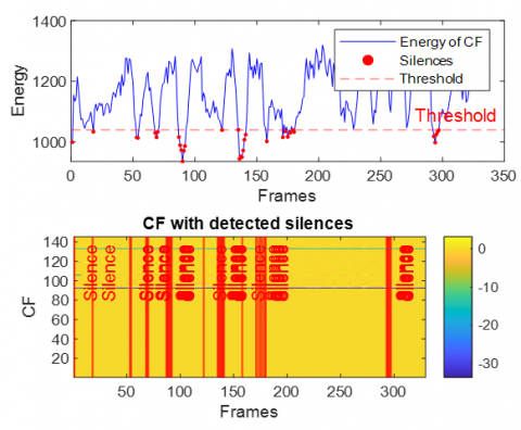
4.3 Combined features and detected silence periods
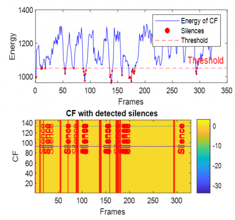
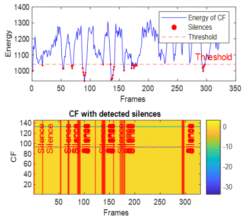
This section presents the results of integrating the extracted acoustic features and the subsequent silence detection process. To illustrate the efficacy of the feature combination and the precision of silence identification, we have traced the energy of the combined feature vectors alongside the detected silent regions. This analysis is performed across various challenging acoustic environments, specifically utilizing data corrupted by White Gaussian noise, babble noise, F16 aircraft noise, factory noise (Factory1), HF-channel noise, and buccaneer noise. The Figures 16-21 provide a visual representation of these energy profiles and the detected silences in case of dispersive system.
In the dispersive case (see Figures 16-21), several general observations can be made regarding the behavior of the Energy of combined features and the performance of the silence detection mechanism. Due to the spreading effect of dispersive environments, the energy of CF exhibits significant fluctuations over time, as even small variations in the input signal (speech+noise) lead to broad changes in the output.
Figure 16. Energy of combined features with detected silence periods in dispersive case with white noise
Figure 17. Energy of combined features with detected silence periods in dispersive case with babble noise
Figure 18. Energy of combined features with detected silence periods in dispersive case with F16 aircraft noise
Figure 19. Energy of combined features with detected silence periods in dispersive case with factory1 noise
Figure 20. Energy of combined features with detected silence periods in dispersive case with Hf channel noise
Figure 21. Energy of combined features with detected silence periods in dispersive case with buccaneer noise
Across Figures 16–21 (white, babble, F-16 aircraft, factory1, HF channel, buccaneer), the energy traces display dynamic patterns with recurrent peaks and troughs. This reflects the non-stationary nature of noisy speech and the influence of dispersive impulse response. Importantly, despite these variations, the silence detection remains effective, accurately aligning with low-energy valleys across all noise conditions. This demonstrates the robustness of the energy-based thresholding approach in reliably identifying silent segments.
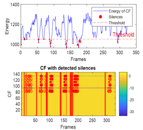
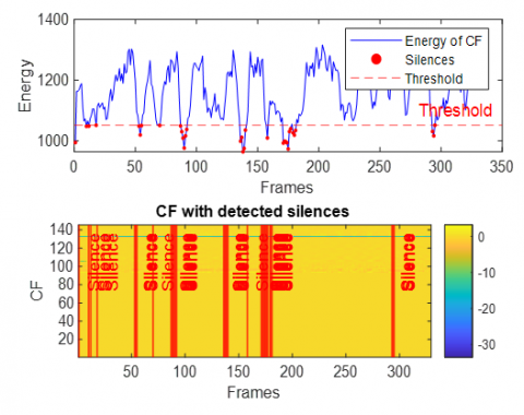
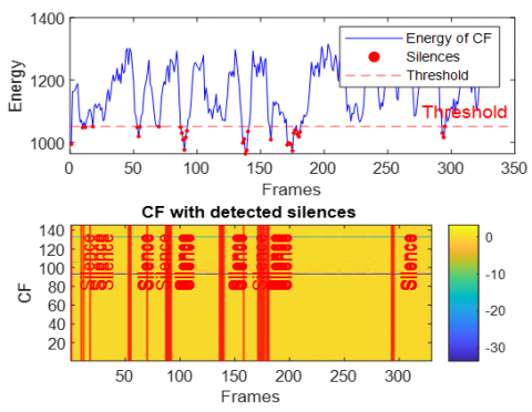
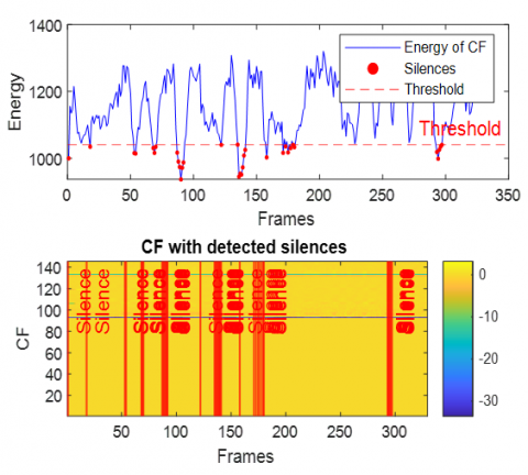
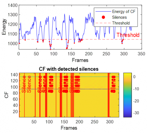
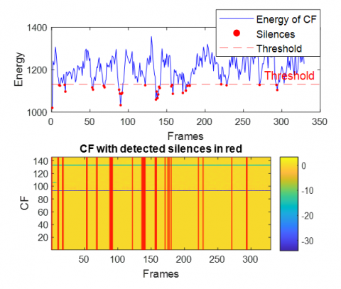
In the second part of these simulations, the analysis is conducted across multiple acoustic environments by incorporating sparse impulse responses to simulate realistic reverberant conditions. The input signals are contaminated with six distinct types of noise. Figures 22–27 present the energy distributions and the corresponding silence-detection performance for each of the six noise types in the presence of sparsely distributed reflections.
In the sparse scenario, the evaluation of the "Energy of CF" and silence detection across various noise environments as presented in Figures 22-27, demonstrates the robustness and consistency of the combined feature extraction and silence detection mechanism. The Energy of CF consistently presents a dynamic pattern with distinct peaks and troughs, reflecting the structure of speech signals embedded in noise. Notably, the energy-based silence detection indicating detected silences successfully captures silent intervals by aligning with low-energy dips in the noisy signal.
Figure 22. Energy of combined features with detected silence periods in sparse case with white noise
Figure 23. Energy of combined features with detected silence periods in sparse case with babble noise
Figure 24. Energy of combined features with detected silence periods in sparse case with F16 aircraft noise
Figure 25. Energy of combined features with detected silence periods in sparse case with factory1 noise
Figure 26. Energy of combined features with detected silence periods in sparse case with Hfchannel noise
Figure 27. Energy of combined features with detected silence periods in sparse case with buccaneer noise
4.4 Estimated VSS by deep learning approach
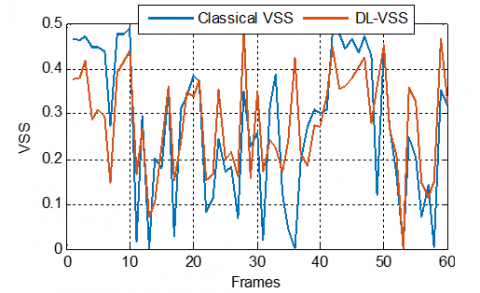
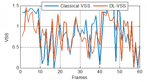
To evaluate the effectiveness of the proposed deep learning-based variable step-size (DL-VSS) strategy, a comparative analysis was conducted against the classical VSS values under two distinct acoustic system scenarios: dispersive and sparse impulse responses. For a fair comparison, both methods were tested using three different values of the maximum step-size parameter: 0.5, 0.9, and 1.5. In each case, the same input signal and noise conditions were applied to isolate the impact of the adaptation mechanism.
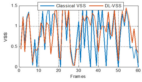
The obtained results presented in Figures 28-30, consistently demonstrate that the proposed Deep Learningbased Variable Step Size (DL-VSS) approach exhibits comparable levels of tracking ability with the classical VSS values in dispersive systems, with clear advantages emerging as the maximum step size increases. At a lower maximum step size of $\mu_{\text {max }}=0.5$, the DL model shows tracking capabilities and curve appears slightly smoother and less oscillatory. As the maximum step size increases to $\mu_{\max }=0.9$, the DL-VSS algorithm begins to show a clearer advantage, maintaining a better balance between fast adaptation and error stability. In the more aggressive scenario of $\mu_{\max }=1.5$, the benefits of DL-VSS become even more pronounced, as its output retains a relatively stable profile despite the high adaptation gain, confirming that the data-driven step-size estimation in DLVSS provides robust and adaptive control crucial for dispersive systems where the filter must adjust to subtle longrange correlations.
Figure 28. DL-VSS evolution compared with classical VSS ones, with $\mu_{\max}$ = 0.5, in dispersive case
Figure 29. DL-VSS evolution compared with classical VSS ones, with $\mu_{\max}$ = 0.9, in dispersive case
Figure 30. DL-VSS evolution compared with classical VSS ones, with $\mu_{\max}$ = 1.5, in dispersive case
Figure 31. DL-VSS evolution compared with classical VSS ones, with $\mu_{\max}$ = 0.5, in sparse case
Figure 32. DL-VSS evolution compared with classical VSS ones, with $\mu_{\max}$ = 0.9, in sparse case
Figure 33. DL-VSS evolution compared with classical VSS ones, with $\mu_{\max}$ = 1.5, in dispersive case
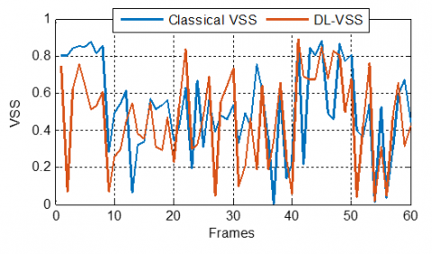
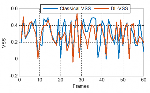
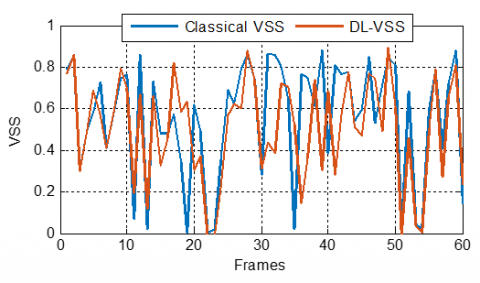
In the sparse case simulations presented in Figures 31-33, a comparison between the classical VSS parameters and the DLVSS one revealed distinct adaptation behaviors across varying $\mu_{\text {max}}$. For $\mu_{\text {max }}=0.5$, the classical VSS exhibits significant and abrupt fluctuations, suggesting an oscillation around the optimal step size, which might indicate a struggle in precisely adapting to the sparse system characteristics. In contrast, the DL-VSS demonstrates a smoother and more controlled stepsize trajectory, implying that the deep learning model effectively learns and exploits the underlying sparsity to achieve stable adaptation.
As $\mu_{\text {max }}$ increases to 0.9 and 1.5, the DL-VSS maintains its less erratic behavior compared to the classical VSS, suggesting a better capability to generalize and adapt even with a broader range of allowed step sizes. The DL-VSS consistently exhibits a more controlled and potentially more optimal step-size adaptation than the classical VSS in sparse environments across all tested maximal step-size values, highlighting its ability to provide stable and robust convergence.
4.5 Objective testing criteria for DL model
To rigorously evaluate the performance of the proposed deep learning model for variable step-size estimation, a set of objective testing criteria was employed. These criteria provide quantitative measures of the model's accuracy, precision, and predictive capability. Specifically, the evaluation relies on the Mean Square Error (MSE), Mean Absolute Error (MAE), and the Correlation Coefficient (R2), each offering distinct insights into the discrepancies between the predicted DL-VSS and classical step-size parameters.
Table 1 presents the objective testing criteria (MAE, MSE, and R2) for the DL-VSS model across varying input Signal-to-Noise Ratio (Input SNR) levels in both dispersive and sparse environments. The MAE, MSE and R2 criteria are employed to confirm the accuracy and reliability of the proposed DL step-size predictor across both dispersive and sparse impulse responses.
Table 1. Objective criteria (MAE, MSE and R2) for DL-model validation across SNRs in dispersive and sparse cases for three Input SNR
|
Types of IR |
Input SNR in dB |
Testing Criteria |
||
|
MAE |
MSE |
R2 |
||
|
Dispersive case |
-6 |
0.1448 |
0.0521 |
0.1204 |
|
-3 |
0.1784 |
0.0516 |
0.1403 |
|
|
0 |
0.1913 |
0.0605 |
0.1800 |
|
|
3 |
0.0504 |
0.1787 |
0.1892 |
|
|
6 |
0.1532 |
0.0402 |
0.3949 |
|
|
Sparse case |
-6 |
0.1291 |
0.0384 |
0.2995 |
|
-3 |
0.1571 |
0.0523 |
0.3613 |
|
|
0 |
0.1450 |
0.0460 |
0.4760 |
|
|
3 |
0.1154 |
0.0251 |
0.6514 |
|
|
6 |
0.1448 |
0.0434 |
0.3955 |
|
In the dispersive case, the DL-VSS algorithm demonstrates its strongest predictive accuracy at 3dB SNR, achieving the lowest MAE (0.0504) and a notably low MSE (0.1787). This indicates that the predicted step-size parameters are closest to the true values under moderately noisy dispersive conditions. However, the correlation coefficient values for the dispersive case are generally low across all SNRs, with the highest being 0.3949 at 6dB SNR. The particularly low R2 values at lower SNRs, such as 0.1204 at -6dB and 0.1403 at -3dB, suggest that while the algorithm can achieve low error metrics at specific SNRs, its overall ability to explain the variance in the true step-size parameters in dispersive environments is moderate, implying challenges in capturing the complex underlying relationships, especially in very noisy conditions.
In the sparse case, the DL-VSS algorithm exhibits superior and more robust performance across the tested SNR range. It achieves its best predictive accuracy at 3dB SNR, boasting the lowest MAE (0.1154) and MSE (0.0251). These errors are consistently lower than those observed in the dispersive case across most SNR levels, indicating that the DL-VSS effectively leverages the inherent sparsity of the system for more precise step-size estimation.
Furthermore, the R2 values in the sparse case are significantly higher than in the dispersive case, peaking at a substantial 0.6514 at 3dB SNR. This high R2 value signifies that the DL-VSS model explains a considerable proportion of the variance in the true step-size parameters, reflecting a strong fit and robust predictive capability, particularly under moderate noise. Even at lower SNRs like -6dB, the R2 (0.2995) is markedly better than its dispersive counterpart, underscoring the model's improved ability to capture relevant relationships in sparse environments
4.6 Acoustic noise reduction performance
To validate the effectiveness of the proposed DL-VSS-FNLMS algorithm for acoustic noise reduction, we conducted a comparative study against the classical FNLMS algorithm with fixed step-size values. This evaluation was carried out under both dispersive and sparse systems, allowing us to assess the generalization ability and robustness of the proposed algorithm across different impulse response types.
The comparison focuses on the time evolution of the estimated speech signal obtained by the classical and proposed algorithms. We also present other results based on system mismatch, output segmental SNR and cepstral distance, for evaluating respectively the convergence speed, speech enhancement quality and distortion level of the enhanced speech. In case of dispersive case, we present the performance of two algorithms in four Figures 34-37, respectively for time evolution, SM, SegSNR and CD.
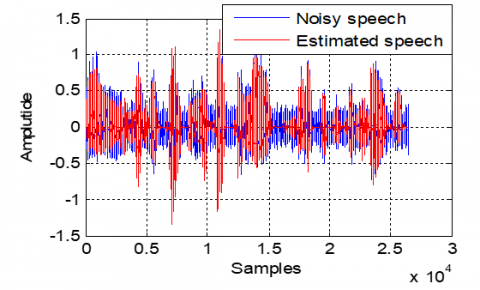
Based on Figure 34, we note that the proposed algorithm is capable of extracting the speech signal and reducing the noise in acoustic dispersive system.
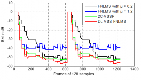
Regarding SM criteria (see Figure 35), and by using an abrupt change in the middle, which simulates the variation of the impulse response, the FNLMS with μ=0.2 shows relatively slow initial convergence with steady-state values between -40 and -50dB. The FNLMS with μ=1.2 converges much faster initially but exhibits a higher and more oscillatory steady-state value, often remaining above -40dB. In contrast, the proposed DL-VSS-FNLMS achieves the fastest initial convergence and consistently the lowest steady-state values, often reaching below -50dB and approaching -60dB, and a good re-convergence in the case of the change of impulse response.
Figure 34. Time evolution of estimated speech signal in dispersive case
Figure 35. SM evaluation obtained by DL-VSS-FNLMS, FNLMS and 2C-VSSF in dispersive case
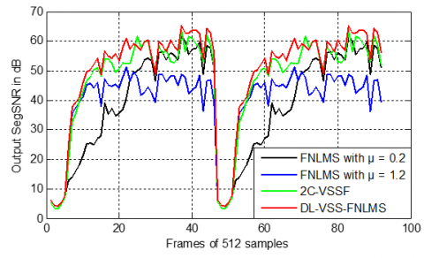
Figure 36. Output SegSNR evaluation obtained by DL-VSS-FNLMS, FNLMS and 2C-VSSF in dispersive case
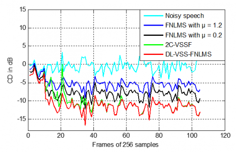
Figure 37. CD evaluation obtained by DL-VSS-FNLMS, FNLMS and 2C-VSSFin dispersive case
Based on Figure 36, the FNLMS with μ=1.2 achieves modest final SNR levels, generally below 60 dB. The FNLMS with μ=0.2 shows higher SegSNR values in some instances, but can be more irregular. The DL-VSS-FNLMS consistently achieves the highest final SNR levels, often exceeding 60dB and at times nearing 65dB, demonstrating its superior ability to enhance speech quality by effectively reducing noise while preserving speech components in dispersive environments.
Based on Figure 37, the CD results in the dispersive case show that the proposed DL-VSS algorithm outperforms the fixed-step-size and classical VSS one. A key finding is that the VSS algorithm produces enhanced speech signals with significantly less speech distortion, making them sound much clearer to a listener.
However, the obtained results of acoustic noise reduction in case of the acoustic sparse system are presented in three Figures 38-41.
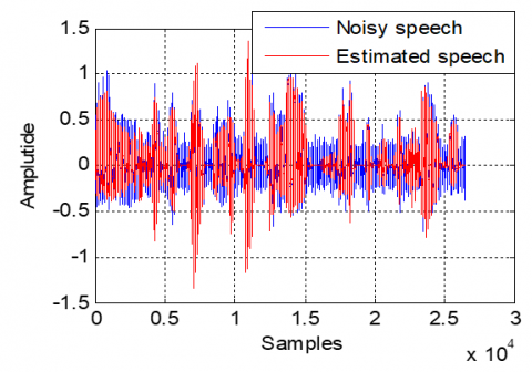
Figure 38 shows that the proposed algorithm significantly reduces the acoustic noise, especially during non-speech segments. During active speech periods, the DL-VSS-FNLMS effectively preserves the speech signal, confirming its capability to perform accurate noise suppression even in systems with sparse impulse responses.
Figure 38. Time evolution of estimated speech signal in sparse case
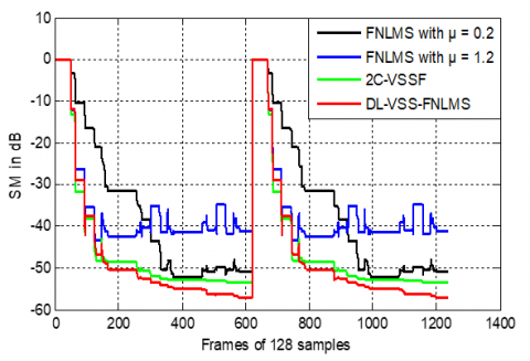
Based on SM presented in Figure 39, the FNLMS with μ=0.2 shows slow convergence and stabilizes at a relatively high mismatch level, typically fluctuating between -45dB and -50dB. The FNLMS with μ=1.2 converges faster but suffers from instability, with its SM oscillating around -35dB to -40dB. In other hands, the proposed algorithm achieves the fastest convergence, reaching SM levels between -55dB and -60dB. the steady-state values obtained by proposed, demonstrating its ability to efficiently exploit the sparsity of the system through dynamic step-size adjustment.
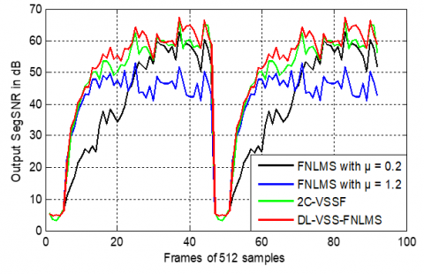
In terms of SegSNR values (see Figure 40), the FNLMS with μ=1.2 yields acceptable but suboptimal values, generally below 50dB, with μ=0.2 shows higher SegSNR in active speech regions due to its faster adaptation, but its results are less stable. The proposed DL-VSS-FNLMS clearly outperforms both, consistently achieving SegSNR values above 65dB, indicating superior noise suppression and speech enhancement.
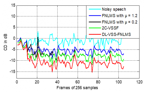
From the CD curves for the sparse IR condition presented in Figure 41, the proposed DL-VSS-FNLMS consistently achieves the lowest cepstral distance both in convergence and steady state compared with fixed-step and classical VSS algorithm.
Figure 39. SM evaluation obtained by DL-VSS-FNLMS, FNLMS and 2C-VSSF in sparse case
Figure 40. Output SegSNR evaluation obtained by DL-VSS-FNLMS, FNLMS and 2C-VSSFin dispersive case
Figure 41. CD evaluation obtained by DL-VSS-FNLMS, FNLMS and 2C-VSSFin dispersive case
4.7 Computational complexity and real-time feasibility
We present in this part the computational complexity and memory usage of a deep learning-based adaptive filter system. The entire system operates on 16kHz audio with a 25ms window and 10ms hop. The proposed technique is composed of three main parts:
Feature Extraction: This initial stage uses a causal 512-point STFT to compute various features like MFCC, GTCC, Mel, Bark, and ERB. It requires approximately 5-6 million MACs/s and has a very low memory usage, less than 0.15MB.
DL Predictor: This component is a 3-layer LSTM network with 64, 64, and 32 neurons. It predicts a scalar value μ(n) from 120-dimensional features. It is the most computationally intensive part, demanding about 9.2 million MACs/s. The model and its state require around 0.35MB of memory for 32-bit floating-point numbers or 0.18 MB for 16-bit integers.
Adaptive Filter: This final stage performs a standard FNLMS/NLMS update with M=128 taps. It requires roughly 4.1 million MACs/s and its memory usage is considered negligible. As seen in Table 2, the total processing workload is approximately 18-20 million MACs/s (Multiply-Accumulate Operations per Second), with a total memory footprint of less than 0.5MB, which is very suitable for real time implementation of the proposed algorithm.
Table 2. Computational complexity and memory usage of the proposed system
|
Component |
Per-Frame Work (16kHz, 25ms Window, 10ms Hop) |
MACs/s at 100fps |
Memory (Runtime) |
|
Feature extraction |
One causal 512-pt STFT reused for MFCC/GTCC/Mel/Bark/ERB + ∆/∆∆ |
≈ 5-6 MMAC/s |
< 0.15 MB |
|
DL predictor |
3-Layer LSTM (64,64,32) on ≈ 120-D features $\rightarrow \mu(n)$ |
≈ 9.2 MMAC/s |
≈ 93k params $\rightarrow$⁓ 0.35MB fp32/ ⁓ 0.18 MB int16 +⁓ 1.3 KB state |
|
Adaptive filter |
Standard FNLMS/NLMS update (shown for M = 128 taps) |
≈ 4.1 MMAC/s |
Negligible |
|
Total |
ــــــــ |
≈ 18-20 MMAC/s |
Model + buffers < ⁓ 0.5MB |
In this paper, we have proposed a novel deep learning-based variable step-size estimation method integrated into a two-sensor Feed-forward NLMS algorithm, effectively enhancing adaptive filtering performance in complex acoustic environments. Utilizing an RNN with stacked LSTM layers and a diverse set of acoustic features (MFCCs, GTCCs, ERB, Bark, Mel), the DL-VSS model demonstrated its ability to dynamically and accurately predict optimal step sizes. The model’s robustness was further supported by reliable energy-based silence detection across varied noise types, which provided critical contextual cues for accurate prediction. Objective criteria (MAE, MSE, R²) validated the predictive strength of the approach, especially in sparse conditions, confirming its efficacy as a data-driven solution for adaptive noise reduction in challenging environments, dispersive and sparse situations. Compared to classical FNLMS with fixed step sizes, the proposed DL-VSS-FNLMS algorithm consistently achieved faster convergence, lower steady-state system mismatch, and improved segmental SNR, reflecting superior noise suppression and speech clarity in both dispersive and sparse conditions. Moreover, it ensured more stable step-size control, particularly in cases where classical methods falter due to large step-size instability.
This study shows that our deep learning model effectively performs simultaneous noise reduction and dereverberation on the NOISEX-92 benchmark, enabling direct comparison with prior work. Nonetheless, the methodology is designed to generalize, and future work will evaluate the model across broader, more diverse datasets to fully assess real-world robustness.
|
MSE |
Mean Square Error |
|
MSD |
Mean Square Deviation |
|
MMSE |
Minimum Mean Square Error |
|
BSS |
Blind Source Separation |
|
SAD |
Symmetric Adaptive decorrelation |
|
VSS |
Variable Step Size |
|
NLMS |
Normalized Least Mean Square |
|
DL-VSS-FNLMS |
Deep Learning VSS-FNLMS |
|
VAD |
Voice Activity Detector |
|
HF |
High Frequency |
|
MFCC |
Mel-Frequency Cepstral Coefficient |
|
GTCC |
Gammatone Cepstral Coefficient |
|
STFT |
Short-Time Fourier Transform |
|
DCT |
Discrete Cosine Transform |
|
ERB |
Equivalent Rectangular Bandwidth |
|
RNN |
Recurrent Neural Network |
|
LSTM |
Long Short-Term Memory |
|
RMS |
Root Mean Square |
|
SNR |
Signal to Noise Ratio |
|
SM |
System Mismatch |
|
Seg-SNR |
Segmental SNR |
|
MAE |
Mean Absolute Error |
|
Greek symbols |
|
|
$\mu_{D L}$ |
Step size estimated by DL model |
|
$\Delta^i$ |
The i-order derivative |
|
$\varepsilon$ |
Regularization parameter |
|
$\lambda_i$ |
Forgetting factor |
|
$\rho$ |
Small regularization parameter |
[1] Benesty, J. (2018). Fundamentals of speech enhancement. Berlin: Springer. https://doi.org/10.1007/978-3-319-74524-4
[2] Wang, T., Guo, H., Ge, Z., Zhang, Q., Yang, Z. (2023). An MMSE graph spectral magnitude estimator for speech signals residing on an undirected multiple graph. Eurasip Journal on Audio, Speech, and Music Processing, 2023(1): 7. https://doi.org/10.1186/s13636-023-00272-z
[3] Borjigin, A., Kokkinakis, K., Bharadwaj, H.M., Stohl, J.S. (2024). Deep learning restores speech intelligibility in multi-talker interference for cochlear implant users. Scientific Reports, 14(1): 13241. https://doi.org/10.1038/s41598-024-63675-8
[4] Li, J., Sakamoto, S., Hongo, S., Akagi, M., Suzuki, Y. (2008). Adaptive β-order generalized spectral subtraction for speech enhancement. Signal Processing, 88(11): 2764-2776. https://doi.org/10.1016/J.SIGPRO.2008.06.005
[5] Sergio, D.P., Diniz, R. (2002). Adaptive Filtering: Algorithms and Practical Implementation, pp. 1-495. https://doi.org/10.1007/978-3-030-29057-3
[6] Abadi, M.S.E., Husøy, J.H. (2008). Selective partial update and set-membership subband adaptive filters. Signal Processing, 88(10): 2463-2471. https://doi.org/10.1016/J.SIGPRO.2008.04.014
[7] Apolinário, J.A., Rautmann, R. (2009). QRD-RLS adaptive filtering. In J.A. Apolinário (Ed.). Springer New York, USA, 1978: 1-350. https://doi.org/10.1007/978-0-387-09734-3
[8] Benallal, A., Benkrid, A. (2007). A simplified FTF-type algorithm for adaptive filtering. Signal Processing, 87(5): 904-917. https://doi.org/10.1016/J.SIGPRO.2006.08.013
[9] Yang, F., Wu, M., Yang, J., Kuang, Z. (2014). A fast exact filtering approach to a family of affine projection-type algorithms. Signal Processing, 101: 1-10. https://doi.org/10.1016/J.SIGPRO.2014.01.030
[10] Benesty, J., Huang, G., Chen, J., Pan, N. (2024). Microphone arrays. Springer Cham, 22: 1-223. https://doi.org/10.1007/978-3-031-36974-2
[11] Kolbæk, M. (2018). Single-microphone speech enhancement and separation using deep learning. AALBORG Universitet. https://doi.org/10.54337/aau300036831
[12] Albataineh, Z., Salem, F.M. (2021). A RobustICA-based algorithmic system for blind separation of convolutive mixtures. International Journal of Speech Technology, 24(3): 701-713. https://doi.org/10.1007/s10772-021-09833-z
[13] Brendel, A., Haubner, T., Kellermann, W. (2023). A unifying view on blind source separation of convolutive mixtures based on independent component analysis. IEEE Transactions on Signal Processing, 71: 816-830. https://doi.org/10.1109/TSP.2023.3255552
[14] Gabréa, M. (2003). Double affine projection algorithm-based speech enhancement algorithm. In 2003 IEEE International Conference on Acoustics, Speech, and Signal Processing (ICASSP'03), Hong Kong, China, pp. I-I. https://doi.org/10.1109/ICASSP.2003.1198928
[15] Bendoumia, R., Djendi, M. (2015). Two-channel variable-step-size forward-and-backward adaptive algorithms for acoustic noise reduction and speech enhancement. Signal Processing, 108: 226-244. https://doi.org/10.1016/j.sigpro.2014.08.035
[16] Djendi, M., Bendoumia, R. (2013). A new adaptive filtering subband algorithm for two-channel acoustic noise reduction and speech enhancement. Computers & Electrical Engineering, 39(8): 2531-2550. https://doi.org/10.1016/j.compeleceng.2013.09.009
[17] Van Gerven, S., Van Compernolle, D. (1995). Signal separation by symmetric adaptive decorrelation: Stability, convergence, and uniqueness. IEEE Transactions on Signal Processing, 43(7): 1602-1612. https://doi.org/10.1109/78.398721
[18] Bendoumia, R. (2024). New two-microphone simplified sub-band forward algorithm based on separated variable step-sizes for acoustic noise reduction. Applied Acoustics, 222: 110069. https://doi.org/10.1016/J.APACOUST.2024.110069
[19] Araki, S., Makino, S., Aichner, R., Nishikawa, T., Saruwatari, H. (2003). Subband based blind source separation for convolutive mixtures of speech. In 2003 IEEE International Conference on Acoustics, Speech, and Signal Processing (ICASSP'03), Hong Kong, China, 5: V-509. https://doi.org/10.1109/ICASSP.2003.1200018
[20] Djendi, M., Bendoumia, R. (2014). A new efficient two-channel backward algorithm for speech intelligibility enhancement: A subband approach. Applied Acoustics, 76: 209-222. https://doi.org/10.1016/j.apacoust.2013.08.013
[21] Liao, C.F., Tsao, Y., Lee, H.Y., Wang, H.M. (2019) Noise adaptive speech enhancement using domain adversarial training. Proceedings of the Annual Conference of The International Speech Communication Association, Interspeech, 2019: 3148-3152, https://doi.org/10.21437/Interspeech.2019-1519
[22] Cheng, G., Liao, L., Chen, K., Hu, Y., Zhu, C., Lu, J. (2023). Semi-blind source separation using convolutive transfer function for nonlinear acoustic echo cancellation. The Journal of the Acoustical Society of America, 153(1): 88-95. https://doi.org/10.1121/10.0016823
[23] Hassani, I., Bendoumia, R., Guessoum, A., Abed, A. (2024). New Variable selected coefficients adaptive sparse algorithm for acoustic system identification. Traitement du Signal, 41(3): 1089-1099. https://doi.org/10.18280/ts.410301
[24] Duttweiler, D.L. (2002). Proportionate normalized least-mean-squares adaptation in echo cancelers. IEEE Transactions on Speech and Audio Processing, 8(5): 508-518. https://doi.org/10.1109/89.861368
[25] Benesty, J., Gay, S.L. (2002). An improved PNLMS algorithm. In 2002 IEEE International Conference on Acoustics, Speech, and Signal Processing, Orlando, FL, USA, 2: II-1881. https://doi.org/10.1109/ICASSP.2002.5744994
[26] Zue, V., Seneff, S., Glass, J. (1990). Speech database development at MIT: TIMIT and beyond. Speech Communication, 9(4): 351-356. https://doi.org/10.1016/0167-6393(90)90010-7
[27] Varga, A., Steeneken, H.J. (1993). Assessment for automatic speech recognition: II. NOISEX-92: A database and an experiment to study the effect of additive noise on speech recognition systems. Speech Communication, 12(3): 247-251. https://doi.org/10.1016/0167-6393(93)90095-3
[28] Hassani, I., Arezki, M., Benallal, A. (2020). A novel set membership fast NLMS algorithm for acoustic echo cancellation. Applied Acoustics, 163: 107210. https://doi.org/10.1016/j.apacoust.2020.107210
[29] Pearce, D., Hirsch, H.G. (2000). The Aurora experimental framework for the performance evaluation of speech recognition systems under noisy conditions. In 6th International Conference on Spoken Language Processing, Beijing, China, pp. 29-32. https://doi.org/10.21437/ICSLP.2000-743
[30] Al-Kindi, M.J., Dunlop, J. (1989). Improved adaptive noise cancellation in the presence of signal leakage on the noise reference channel. Signal Processing, 17(3): 241-250. https://doi.org/10.1016/0165-1684(89)90005-4
[31] Alilouche, A., Bendoumia, R., Hassani, I., Albu, F. (2025). New sub-band proportionate variable nlms algorithm for the identification of acoustical dispersive-and-sparse impulse responses. Traitement du Signal, 42(3): 1293-1307. https://doi.org/10.18280/ts.420307