Haoyang Fan![]() | Yanming Zhao*
| Yanming Zhao*![]() | Guoan Su
| Guoan Su![]() | Tianshuai Zhao
| Tianshuai Zhao![]() | Songwen Jin
| Songwen Jin![]()
© 2023 IIETA. This article is published by IIETA and is licensed under the CC BY 4.0 license (http://creativecommons.org/licenses/by/4.0/).
OPEN ACCESS
Regarding the classification of 3D point clouds, existing Graph Convolution Networks (GCN) often fail to effectively learn the correlation of visual features of different scales under the condition of multi-view (multi-domain), thus the features learnt by models are not as varied and the classification accuracy is usually limited. In view of these defects, this paper proposed a Multi-View Deep Visual Adaptive Graph Convolution Network (MVDVAGCN) which integrates the theory of visual selective attention with the graph convolution calculation method and inherits the advantages of the idea of rasterization. In the paper, the deep learning technology, the idea of multi-view, and the VAGCN were combined to establish three GCN models which were then applied to the classification of 3D point clouds and attained good results. Then the parameters set for the proposed algorithm were verified based on the ModelNet40 dataset, the recognition performance and geometrical invariance of the proposed algorithm and a few reference algorithms including VoxNeT, PointNet, PointNet++, DGCNN, KPConv3D-GCN, Dynamic Graph CNN, and 3D_RFGCN, were tested, and the results proved the feasibility, recognition performance, and geometrical invariance of the proposed algorithm.
visual selective attention, graph convolution, multi-view, adaptive, rasterization
The development of RGBD and LIDAR sensing technologies makes the data acquisition of 3D point clouds more accurate, the accurate 3D point cloud database has made the 3D point cloud processing algorithm a hot spot of current research, and good results have been attained in fields such as augmented reality, UAV, and autopilot [1-3].
3D point cloud data are unstructured, unordered, and denser in closer positions and sparse in farther positions. The spatial topological structure of 2D data raster enables the conventional structure-related convolution technology to better learn the features of 2D spatial data; however, the data of 3D point clouds do not have obvious topological structure information and they are unstructured, therefore, the conventional structured convolution technology doesn’t have the ability to learn the features of 3D point clouds directly, so solve this problem, researchers adopted the method of point cloud data rasterization and the direct point cloud data processing algorithm to realize the learning of point cloud features, wherein the graph convolution algorithm is an important approach for this research.
Rasterization methods include orthogonal rasterization and polarized rasterization, wherein orthogonal rasterization determines the spatial topological relationship inherent in the data through artificial orthogonal rasterization which rasterizes the unstructured point cloud data into structured data with fixed neighborhood relationship, in this way, the conventional structured convolution technology is improved and its application has been expanded. The voxel filtering method [4-6] is one representative orthogonal rasterization method which has sound mathematical foundations, theories, and methodologies, it can realize the rasterization of spatial point clouds, and directly apply the conventional structure-related convolution technology to the raster data and learn the structural features of point cloud data.
Polarized rasterization [7-9] (namely the multi-view method) centers on 3D subjects and rasterizes them from multiple polarization directions (views) with a fixed view distance as the radius and then forms a 2D data view sequence, in this way, it rasterizes the unstructured 3D point cloud data and reduces the dimensionality into a 2D polarized direction image sequence, then the conventional structure-related convolution technology can be applied directly to the image sequence to learn the point cloud features, since the mathematical foundations, theories, and methodologies of polarized rasterization are complete, so its application is simple and easy.
These two kinds of rasterization methods could be realized by different mathematical processing methods and they have good theoretical and research values in some application fields, however, they have a few common defects as well: (1) The precision of rasterization is determined manually rather than set self-adaptively according to the features of the dataset, some rasterized point cloud data have division ambiguity and information loss problems, which can lead to deficiencies in the completeness and purity of point cloud features; (2) The complex spatial topological relationship generated by the precision of manual rasterization increases the spatial complexity of the algorithm and slows down the performance of the algorithm. Polarized rasterization realizes spatial dimension reduction, and the original spatial topological structure information is lost, so it can not effectively re-construct the scenes or realize scene segmentation. Although some improvements have been made to the algorithm [10, 11] later, still the essential problem with manual rasterization hasn’t been solved yet.
The idea of manual rasterization destroys the original spatial structure of point cloud and changes the spatial topological relationship and the topological selectivity of point cloud data. Topological selectivity means that the polarization direction of cloud data distribution is selectable and the probability of polarization distribution is determined, and it can be measured qualitatively and adaptively by clustering. Inspired by the theory of visual selective attention, the spatial topological relationship and topological selectivity of point cloud data are defined as the visual topological selectivity of point cloud data, the definition and expression can be realized by applying the theory of receptive field. The features can be perfectly expressed under the condition of sufficient sampling, and these features are geometrically invariant.
Then on this basis, the direct point cloud processing method has been proposed, which has changed the problems with rasterization processing. This method mainly contains the definition of graph convolution algorithm and its realization on 3D point cloud data, wherein the two most important deep learning methods are PointNet [12], PointNet++ [13], and the subsequent improved algorithms of the model [14-16].
The PointNet algorithm [12], which has integrated the T-net algorithm, the point-by-point Multi-Layer Perception (MLP) algorithm, and the channel-by-channel max pooling method, can learn the global features of 3D point cloud data and solve the disorder problem with data, but the algorithm itself has the shortcoming of inablity to learn the local features of point clouds. To solve this shortcoming, the PointNet++ algorithm [13] adopted two processing methods, Multi-Scale Grouping (MSG) and Multi-Resolution Grouping (MRG) to realize data sampling under the condition of different scales and resolutions, moreover, the PointNet algorithm was applied to the cloud of sampling points to extract all features of sampling point cloud, namely the local features of the original 3D point cloud, and this has solved the problem of PointNet algorithm in ignoring local features. Since then, improvements have been made to the algorithm in terms of global features, local features and feature invariance to enhance its application capability.
However, the above algorithm has ignored the spatial topological structure of 3D point cloud data, and this structure has obvious graph structure, so the representation of point cloud data based on graph structure and its 3D graph convolution analysis algorithms have become a new research direction for 3D point cloud [17-20], and some progresses have been made in terms of research and application. Inspired by the PointNet++ algorithm, this method learns the local spatial features (namely the global features of sample set) of the original data of point cloud. The DGCNN algorithm [21] can form sub point sets by identifying the nearest neighbor of 3D points in the feature space and then extract features through edge convolution operations to construct the local graph structure. Shen et al. [22] expanded the idea mentioned above and further learnt the spatial topological information during the process of feature clustering. The RS-CNN [23] (Relation-shape CNN) used weighted sum of neighbor node features, wherein each weight was learnt by MLP based on the geometric relationship between two points. These works are all attempts to learn the local topological features of 3D point cloud. The 3D-GCN [24] adopted a deformable 3D kernel to learn the information of 3D point cloud, it processed different-scale information based on the max pooling method to solve the unordered and unstructured data of point cloud, and the idea of universal model was proposed.
Although the above mentioned methods have attained good theoretical and practical research results in terms of graph representation and graph convolution, still there are a few problems: (1) There isn’t a universal 3D graph convolution method proposed with the theory of selective attention for primate and the graph convolution technology taken into consideration; (2) There isn’t a universal 3D graph convolution algorithm that inherits the merits of polarized rasterization and can realize self-adaptation according to the distribution features of point cloud data; (3) There isn’t an optimized universal and self-adaptive 3D graph convolution algorithm that combines the visual hierarchical and serial processing method with deep learning to realize the deep-level abstract learning of visual information; (4) The existing methods haven’t combined with the correlation of different-scale visual under the condition of multi-view (multi-domain), thus the model learning features are not as varied and the classification accuracy is usually limited. In view of these, this paper proposed the said multi-view VAGCN, inspired by the theory of selective attention of primate, our method effectively integrates the theory of selective attention, the graph convolution technology, the polarized rasterization method, the deep learning technology, the visual hierarchical serial processing method, and the correlation analysis of different visual features of multiple views, our paper realized a multi-view deep-level visual selective attention feature learning algorithm and applied it to the classification of 3D point cloud data.
Innovations of this paper include:
(1) This paper proposed the VAGCN algorithm (VAGCN is the abbreviation of Visual Adaptive Graph Convolution Network) that can effectively and adaptively learn the global and local features of 3D point cloud.
(2) This paper integrated the deep learning theory with the VAGCN algorithm to propose the DVAGCN algorithm (DVAGCN is the abbreviation of Deep VAGCN) which can learn the deep-level abstract features of 3D point cloud at different depths and scales and form complete and deeply integrated features.
(3) To ensure the completeness and purity of the deeply integrated 3D point cloud features, based on DVAGNN, this paper proposed the MVDVAGCN (MVDVAGCN is the abbreviation of Multi-View Deep VAGCN) which can learn the visual features of multi-view 3D point cloud and their correlation to form the optimal view and realize optimal recognition performance.
(4) Definition of models related to the algorithm. Inspired by the link processing method of visual information of the primate, this paper took the VAGCN as the core to propose a single link recognition model and two double link recognition models on this basis, then, experiments were carried out to verify the feasibility of the three models and the consistency of their recognition performance.
(5) Innovation in the experiment. On the ModelNet40 dataset, the algorithm parameters were set in the experiment and the correctness and feasibility of the algorithm were verified based on optimal parameters. During the experiment, the proposed algorithm was compared with conventional algorithms, its advantages in recognition performance and geometrical invariability were proved.
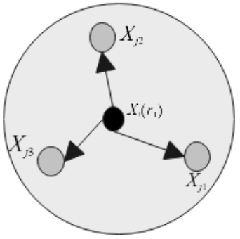
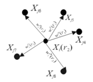
The visual attention of primate has the selective feature, in the visual space of primate, the visual selectivity indicates that the function of visual cells has the feature of “similar receptive fields distribute nearer and different receptive fields distribute farther”, visual nerve cells realize their visual function through the receptive fields, so receptive fields with similar functions have a nearer spatial distribution, while receptive fields with different functions have a farther distribution. Receptive fields directly characterize the visual features of subject and their distribution law, that is, the visual features of subjects are learnt and expressed via the receptive fields of visual nerve cells. Visual selectivity exhibits a pattern that visual features with similar functions are distributed in the close visual field and the visual features with different functions are distributed in the remote visual field.
Thus, in case that the point of sight p is determined, the distance of sight R determines the attributes of receptive fields within the visual space and the quantity and quality of visual features that can be learned, so there is an optimal or sub-optimal sight distance R that makes the visual features of receptive fields similar within the visual field with p as the center, it can be considered as visual functional group which can be represented by a family of functions. The definition of visual space is:
$\Gamma\left(R, P_i\right)=M_P(R)=M_i^j(R)=\left\{P_j \mid\left\|P_j-P_i\right\| \leq R, i, j=1,2,3, \ldots\right\}$ (1)
$\Gamma(R, P)$ represents the area of visual space with $p$ as the point of sight and $R$ as the radius of sight distance, within this area, visual nerve cells have similar receptive fields; this area is a super-sphere; and $\Gamma(R, P)$ is an infinite collection. In 3D point cloud applications, the number of elements in the collection is experimentally determined based on the characteristics of dataset, the degree of sampling, and the method of spatial rasterization.Inspired by the theory of selective attention of primate, in space $\Gamma(R, P)$, receptive fields in the visual space are consisted of the local features and global features of receptive field cells in the space, so the receptive field of 3D space is defined as:
$\operatorname{spatial}_{-} R F_{p_i}^{j k}(R)=\left(x, y, z, \alpha, \beta, \gamma, \rho, \tau, \triangle, \varphi, w_i^{j k}\right)$ (2)
In a visual space, coordinates of sight point $p_i$ describe the local features of visual information; the spatial distribution parameters $\alpha, \beta, \gamma, \rho$ describe the global visual features under this condition, wherein $\alpha, \beta, \gamma$ represent the angles between vector $\overrightarrow{P_l P_j}$ and axes $x, y, z$ (the feature distribution directions); $\rho$ represents the distance from the origin in polar coordinates (the feature distribution position); parameter $\Delta$ represents the degree of changes of point set in directions $(\alpha, \beta, \gamma)$ within the area when the distance from pole $\rho$ changes (the change rate of the number of receptive field cells in the area), therefore, the spatial receptive field spatial_RF is a fusion of local and global features, and this function can better learn and express the visual information of point set; function $\varphi$ represents the degree of polarized rasterization in the visual space, in any direction, the number of polarized raster is $N u m=360 / \varphi$, $w_i^{j k}$ represents the number of receptive fields in the area, and it's called the exuberance degree of receptive field.
$\begin{gathered}w_i^{j k}=\Delta \rho=\Delta \sqrt{r}=\Delta \\ \sqrt{\left(x_j-x_i\right)^2+\left(y_j-y_i\right)^2+\left(z_j-z_i\right)^2} \leq R\end{gathered}$ (3)
Inspired by the theory of selective attention, there is $\lim \left\|\overrightarrow{P_i P_j}\right\| / R=0$, that is, the visual nerve cells in space $\Gamma(R, P)$ have the same receptive field, and the receptive field space formed by clustering is very small.
Therefore, according to above definition, the universal receptive field space of point cloud is illustrated in Figure 1.
a) Local description of point cloud receptive field
b) Global description of adaptive point cloud receptive field based on clustering
c) Global description of adaptive point cloud receptive field when the cluster radius is 1
Figure 1. Spatial receptive fields based on 3D point cloud
Algorithm design in this paper includes three parts: the VAGCN, the DVAGCN, and the MVDVAGCN. Details are given below.
3.1 VAGCN (Visual Adaptive Graph Convolution Network)
Inspired by the theory of selective attention in high-dimensional space, the visual selectivity of highdimensional space was combined with the graph convolution algorithm to propose the VAGCN; inspired by the method of polarized rasterization, in area $\Gamma(R, P)$, according to the features of point cloud data themselves, the clustering method was adopted to determine the degree of polarized rasterization of area $\Gamma(R, P)$ to realize the VAGCN algorithm, pseudo codes of VAGCN are given in Table 1.
Table 1. Pseudo codes of VAGCN algorithm
|
Input: point cloud data; hyper-parameter R; observation point P |
|
Produce: S1: Partition of space neighborhood. With point p as the center and hyper-parameter R as radius, a hyper-sphere spatial neighbor $M_i^j(R)$ is formed. S2 Adaptive polarization of rasterization. In the hyper-sphere spatial neighbor $M_i^j(R)$, the clustering algorithm is executed to determine the degree of polarized rasterization and realize the rasterization of hyper-sphere spatial neighbor $M_i^j(R)$. S3: Feature extraction of adjacent nodes. The MLP method is adopted to extract information about the topological correlation between point $p_i$ and its adjacent node $p_j \cdot w_i^{j k}=h\left(x_i, y_i^{j k}\right)=M L P\left(x_i, y_i^{j k}\right)$. S4: Feature convergence and update: use formula $\bar{X}_l=\sum_{j k \in M_i^{j k}} \varphi\left(w_i^{j k}\right)=\sum_{j k \in M_i^{j k}} M L P\left(w_i^{j k}\right)$ to converge and update the features of node $p_i$. |
|
Output: Graph convolution result of point p in neighbor $M_i^j(R)$. |
Figure 2. Model modules based on VAGCN
According to the VAGCN algorithm, several modules were built, as shown in Figure 2.
According to above algorithm, the VAGCN algorithm can be visualized as shown in Figure 3.
a) Visual field selection ($M_i^j(r)$)
b) Adjacent node feature extraction ($\left(w_i^{j k}=h\left(x_i, y_i^{j k}\right)=\operatorname{MLP}\left(x_i, y_i^{j k}\right)\right.$)
c) Overall visual feature extraction of adjacent nodes
d) Visual information convergence
Figure 3. Visualized description of VAGCN algorithm
3.2 DVAGCN (Deep Visual Adaptive Graph Convolution Network)
The visual information processing of primate is a process of hierarchical and serial processing, the high-level abstraction of visual features is achieved from bottom up, low-level visual features are processed at bottom, and high-level visual features are abstracted and learnt gradually in serial links. This processing theory is the basis of neurophysiology in deep learning [25-27], and the theories and techniques of deep learning are concrete realization of this method. Therefore, this paper combined VAGCN with deep learning to extract abstract visual features of different depths and form complex visual features, so as to improve the abilities of extracting and expressing the visual features. Pseudo codes of the DVAGCN algorithm are given in Table 2.
The 3D point cloud classification model based on DVAGCN algorithm is shown in Figure 4.
Table 2. Pseudo codes of the DVAGCN algorithm
|
Input: point cloud data; hyper-parameter R; observation point P; network depth parameter L. |
|
Produce: S1: Initialize the network depth control parameter NumL, NumL=1; S2: Execute algorithm $D V A G C N^{N u m L+1}=V A G C N^{N u m L}(P C D, R, P)$ and operation $N u m L=N u m L+1$. S3: When network depth control parameter NumL $\leq$ Network depth parameter $L$, algorithm jumps to S2, otherwise the DVAGCN algorithm terminates. |
|
Output: visual features of different depths and their fused features. |
Figure 4. The 3D point cloud classification model based on DVAGCN algorithm (Model 1)
3.3 MVDVAGCN (Multi-View Deep Visual Adaptive Graph Convolution Network)
Due to the influence of super-parameter $R$, the DVAGCN algorithm has following limitations: (1) If the value of parameter $R$ is too small, visual field $M_i^j(R)$ will be limited, which can result in loss of key points, so the completeness of the visual features of set $M_i^j(R)$ is deficient; (2) If the value of parameter $R$ is too large, since there are too many visual nerve cells with different functions in visual field $M_i^j(R)$, the purity of the visual features of set $M_i^j(R)$ is deficient; therefore, there is an optimal or sub-optimal area problem; in terms of feature extraction, it exhibits as the adaptive feature extraction in multiple consecutive visual fields to attain optimal or sub-optimal global or local spatial features, so as to optimize the selection and extraction of features and solve the shortcomings of the VGCN algorithm. Pseudo codes of the MDDVAGCN algorithm are given in Table 3 .
The processing flow of the MVDVAGCN algorithm is described in Figure 5.
Table 3. Pseudo codes of the MDDVAGCN algorithm
|
Input: point cloud data; hyper-parameter set R; observation point P (set P is the triplet of continuous natural number); Network depth parameter L |
|
Produce: S1: Algorithm initialization: $N u m P=\|R\|$, count of visual fields $i=1$. S2: Start GPU and learn the visual features of different visual fields $R_i \in R$ in parallel; $F_{M V D V A G C N}(i)=\operatorname{MVDVAGCN}\left(P C D, R_i, P\right)$ S3: Multi-view feature fusion $H\left(D V A F_{M V D V A G C N}(i) G C N(i)\right)$, wherein $H(\cdot)$ is the feature fusion function. |
|
Output: visual features of different depths and their fusion features. |
a) 3D point set $M_i(r)$
b) Generation of field $M_i\left(r_1\right)$
c) Feature generation of field $r_1$
d) Feature convergence of field $r_1$
e) Generation of field $M_i\left(r_2\right)$
f) Feature generation of field $r_2$
g) Feature convergence of field $r_2$
h) Generation of field $M_i\left(r_3\right)$
i) Feature generation of field $r_3$
j) Feature convergence of field $r_3$
Figure 5. Processing flow of the MVDVAGCN algorithm
3.4 Two models based on MVDVAGCN algorithm
Because the feature fusion function may be in different model positions, so two different models can be developed for a same algorithm, the model is given in Figure 6 and Figure 7.
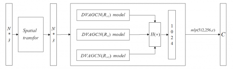
(1) Fusion model before the classification of different-scale visual features.
Figure 6. Classification model of feature fusion based on MVDVAGCN (Model 2)
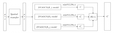
Figure 7. Classification model of recognition result fusion based on MVDVAGCN (Model 3)
In Figure 6, Function $H(\mathrm{o})$ is used to fuse the local and global spatial correlation features of 3D point cloud in multiple visual fields, in experiment, it can be realized by MLP or other algorithms such as the Max Pool.
$H(\mathrm{o})=\operatorname{MLP}\left(\operatorname{MVDVAGCN}\left(\mathrm{R}_i\right)\right)$ or $\operatorname{MaxPool}\left(\operatorname{MVDVAGCN}\left(R_i\right)\right)$ (4)
(2) Fusion model after classification of different-scale visual features.
In Figure 7, Function $H(\mathrm{o})$ is used to calculate the local and global spatial correlation features of 3D point cloud at different sight distances. In experiment, it can be realized by MLP or Max Pool or other algorithms.
$H(o)=M L P\left(\operatorname{class}\left(\mathrm{R}_i\right)\right)$ or $\operatorname{MaxPool}\left(\operatorname{class}\left(R_i\right)\right)$ (5)
Here, the Max Pool algorithm had learnt the global maximum of different visual field features, it is a global feature, while the content of feature details had been ignored, and the time complexity was low. The MLP algorithm had learnt the fusion features of different visual field features, which include the correlation of different-type features, therefore, the features were more representative, but the time complexity of feature fusion was high.
4.1 Dataset
On dataset ModelNet40 [5], the classification performance of the proposed models were tested, this dataset contains categories of shapes that haven’t been spotted before prediction. 12311 raster CAD models of 40 categories are included in the dataset. In this study, 9843 raster CAD models were selected for the training of classification models, and the rest 2468 raster CAD models were used for the tests of classification models. The experiment drew on the settings of the experiment of Qi et al. [12, 13], 1024 points were uniformly sampled from each model raster surface to form an input point cloud dataset, and the coordinates of sampling points $(x, y, z)$ were adopted. In the training process, the input point cloud data were increased through geometrical invariance.
4.2 Model structure and parameter setting
Models applied to 3D point cloud classification in this study include Model 1, Model 2, and Model 3. Model 1 is the basis of the other two models, Models 2 and 3 are the extended expressions of Model 1 in different visual fields. Therefore, the setting of main parameters is mainly about Model 1. In our experiment, the depth of model structure was 4 layers, and parameters of each layer were set as (64, 64, 128, 256). Breadth (namely the multi-view) of the model was 3 columns, which means that the model performs visual feature learning in three consecutive visual fields. Experimental results show that, the breath set $R=\left\{R_1, R_2, R_3\right\}$ is a set of continuous natural numbers, wherein $R_{i 1} \in[20,40]$. The models adopted the method of shortcut connections to realize multi-scale visual feature extraction under different depths, and used the MLP of shared weight to converge multi-depth features to attain a 256-dimensional feature set with depth completeness. The Max/Sum pool algorithm was used to learn the optimal features of 3D point cloud, and two FCs were used to realize the formation of 512 and 256 dimensional features. Moreover, Dropout=0.5 was also adopted for feature elimination, and the model adopted LeakReLu and Batch Normalization for training; the model training parameters were set as: SDG=0.1, learning rate=0.001, batch normalization momentum was 0.9, and data batch size was 32.
4.3 Classification performance of proposed models
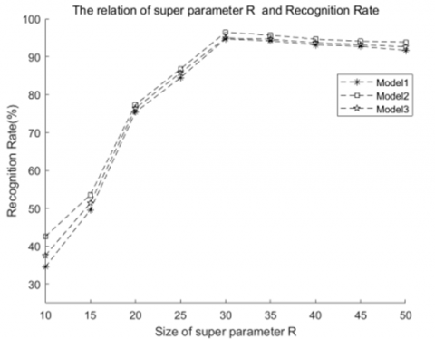
Based on the dataset defined in Section 4.2 and preset model parameters, the relationship between the classification performance of three proposed models and the hyper-parameter R was studied experimentally, and the results are shown in Figure 8.
Figure 8. Relationship between hyper-parameter R and model recognition rate
Experimental results show that within the natural number range of hyper-parameter $R \in[10,50]$, as the $R$ value of visual fields increased, the recognition performance of the three models increased first and then decreased slowly. When $R=R_{\max }=30$, the recognition performance of the three models reached their maximum values $(94.63,96.37,94.88)$, and the rank of recognition rates was $\eta_{\text {Model } 1} \leq$ $\eta_{\text {Model3 }} \leq \eta_{\text {Model2 }}$. The experimental results have verified that the proposed algorithms are feasible and have good classification performance.
Cause of such changes is: within the definition range of the $R$ value of visual fields, with the increase of $R$, the number of 3D point clouds in $M_i^j(R)$ increased, the visual features learnt by models gradually become more complete, and the recognition performance of models showed an increasing trend; when $R=R_{\max }=30$, the visual features learnt by models were complete, and the recognition performance of models reached the maximum; when $R \geq R_{\max }$, the number of 3D point clouds in $M_i^j(R)$ increased gradually, but the number of $3 \mathrm{D}$ point clouds that are not in this category of receptive fields increased as well, although the visual features learnt by models were complete, their purity was deficient, therefore the recognition performance of the models declined a little bit.
Therefore, the optimal interval of visual field $R$ of proposed models is $R \in[20,40]$, and the classification performance of the algorithm in this interval is listed in Table 4.
Table 4. Relationship between the optimal classification performance of models and the value of hyper-parameter R
|
R Model |
20 |
25 |
30 |
35 |
40 |
|
Model1 |
79.80 |
87.62 |
94.63 |
92.36 |
92.23 |
|
Model2 |
81.31 |
88.85 |
96.37 |
95.27 |
94.66 |
|
Model3 |
80.32 |
87.31 |
94.88 |
93.51 |
93.12 |
Relationship between the adaptive polarized rasterization parameter $\varphi$ and the recognition performance of proposed algorithms is:
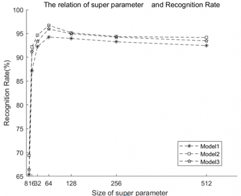
According to the relationship between hyper-parameter R and model recognition rate, it’s selected that R=30, then based on the calculation results of adaptive polarized rasterization parameter in the experimental process, the relationship between adaptive polarized rasterization parameter $\varphi$ and the classification performance of proposed algorithm models was plotted, as shown in Figure 9.
Performance comparison between different algorithms:
Figure 9. Relationship between adaptive polarized rasterization parameter $\varphi$ and the recognition performance of proposed algorithms
Experimental results show that the relationship between the adaptive polarized rasterization parameter and the recognition rate of proposed algorithms exhibits a trend that the algorithm performance increased first and decreased slowly later as the polarized rasterization parameter grew. When $\varphi=\varphi_{\max }=128$, the algorithm recognition rate reached the maximum $\eta=96.36$, the reason is that with the increase of the degree of rasterization, the partitioning of $M_i^j(R)$ was more consistent with visual selective attention, and the point cloud data contained in $M_i^j(R)$ had better completeness and purity; when $\varphi=\varphi_{\max }=128$, point cloud data in $M_i^j(R)$ reached the optimal effect of visual selective attention, those point clouds contained in it had the best completeness and purity, and the model reached the highest classification performance; when $\varphi>\varphi_{\max }$, the completeness of point clouds in $M_i^j(R)$ was deficient, and the recognition performance of the algorithms declined slightly.
Above experimental results show that when hyper-parameter $R \in[20,40]$ and polarized rasterization parameter $\varphi \in$ {128 256 512 1024}, in the beginning, the recognition rate of models was within the optimal range and could meet the requirements of actual applications.
4.4 Advantages of proposed algorithms
On the experimental dataset, in case of a hyper-parameter R=30 and a polarized rasterization parameter $\varphi=128$, the classification performance of proposed models was compared with a few conventional algorithms, and the results are given in Table 5.
Table 5. Algorithm performance comparison
|
Name of Algorithms |
Mean Class Accuracy |
Overall Accuracy |
|
3D SHAPENETs [5] |
77.31 |
84.77 |
|
VoxNeT [28] |
83.03 |
85.92 |
|
VRN (SINGLE VIEW) [29] |
88.07 |
-- |
|
VRN (MULTIPLE VIEWS) [30] |
91.38 |
-- |
|
ECC [31] |
83.23 |
87.41 |
|
PointTNet [12] |
86.03 |
89.21 |
|
PoinTNet++ [13] |
-- |
90.77 |
|
KD-NET [32] |
-- |
90.66 |
|
PointCNN [33] |
88.16 |
92.24 |
|
PCNN [34] |
-- |
92.33 |
|
Dynamic Graph CNN [21] |
90.26 |
93.46 |
|
3D_RFGCN [35] |
91.89 |
94.01 |
|
Model 1 |
88.62 |
94.63 |
|
Model 2 |
89.81 |
96.44 |
|
Model 3 |
89.12 |
94.88 |
The experimental results in Table 2 show that: in case of a hyper-parameter R=30 and a polarized rasterization parameter $\varphi=128$, the average recognition performance of proposed models was much higher than that of most reference algorithms, and the proposed models outperformed other algorithms in terms of optimal recognition performance, therefore, among these 3D point cloud classification algorithms, the proposed algorithms showed good advantages in classification performance.
In addition, the selected algorithms shown in Table 2 are highly representative in terms of point cloud processing, the reference algorithms include the rasterization method [5, 28-30], direct processing method [12, 13], convolution processing method [33, 34], graph convolution processing method [21], and graph convolution method based on visual computing [35]. The 3D point cloud processing technology was explained from several aspects and the experimental results indicate that these algorithms exhibited good classification performance on the dataset adopted in this study; the classification performance of the graph convolution algorithm was the best, the direct processing method performed well, followed by the early rasterization method.
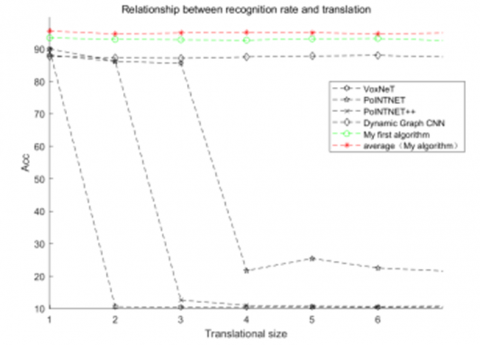
4.5 Visual invariance of models
On the dataset in this paper, in case of a hyper-parameter R=30 and a polarized rasterization parameter $\varphi=128$, the invariance of models was studied experimentally, and the results are shown in Figure 10.
a) Translation vs recognition rate
b) Scale vs recognition rate
c) Rotation vs recognition rate
Figure 10. Relationship between invariance and performance
The experimental results show that the proposed model performed good in terms of invariance under the conditions of small-scale translation, scaling, and rotation; compared with conventional algorithms, their geometric invariance is better.
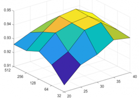
4.6 Recognition performance consistency of different models
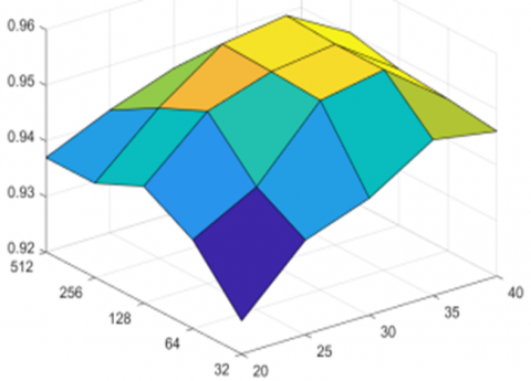
On the dataset in this paper, in case of a hyper-parameter $R \in[20,40]$ and a polarized rasterization parameter $\varphi \in$ {32, 64, 128, 256, 512}, the consistency of the recognition performance of proposed models was studied experimentally, and the results are shown in Figure 11.
a) Recognition performance of Model 1
b) Recognition performance of Model 2
c) Recognition performance of Model 3
Figure 11. Consistency of the recognition performance of proposed models
Inspired by the theory of selective attention of primate, this paper proposed the MVDVAGCN (Multi-View Deep Visual Adaptive Graph Convolution Network) algorithm combining with the advantages of adaptive polarized rasterization algorithm. In the paper, three classification models were designed for multiple visual fields, and were applied to the processing of 3D point cloud. Based on the ModelNet40 dataset, the setting of algorithm parameters was studied, the recognition performance of the proposed algorithm and a few reference algorithms including VoxNeT, PointNet, PointNet++, DGCNN, KPConv3D-GCN, Dynamic Graph CNN and 3D_RFGCN were compared, and the geometric invariance of the proposed algorithm was verified. Experimental results suggest that, the proposed algorithm is correct and feasible; compared with conventional algorithms, the proposed algorithm model has better recognition performance, and its geometric invariance is stable in case of small variations.
In the future, the algorithm will be optimized in two aspects to improve its performance:
(1) Further optimize the parameter setting and performance of the algorithm based on the connection number and type of human visual nerve cells.
(2) Explore the attention mechanism and selective attention consistency and use experiments to prove the conclusion.
This work is supported by the Key R&D Projects in Hebei Province of China (Grant No.:19210111D); the Science and technology planning project of Hebei Province of China (Grant No.:15210135); The social science foundation of Hebei province of China (Grant No.: HB18TJ004 and Grant No.: HB21YS014); The Higher Education Teaching Reform Research and Practice Project of Hebei Province (Grant No.: 2019GJJG510). The Special project of sustainable development agenda innovation demonstration area of the R&D Projects of Applied Technology in Chengde City of Hebei Province of China (Grant No.: 202205B031 and 202205B089). The Introduce intellectual resources Projects of Hebei Province of China in 2023 (The depth computing technology of double-link based on visual selectivity).
[1] Zhu, Y.K., Mottaghi, R., Kolve, E., Lim, J.J., Gupta, A., Li, F.F., Farhadi, A. (2017). Target-driven visual navigation in indoor scenes using deep reinforcement learning. In 2017 IEEE International Conference on Robotics and Automation (ICRA), Singapore, pp. 3357-3364. https://doi.org/10.1109/icra.2017.7989381
[2] Shen, X.K., Stamos, I. (2020). Frustum VoxNet for 3D object detection from RGB-D or Depth images. In Proceedings of the IEEE/CVF Winter Conference on Applications of Computer Vision, Snowmass, CO, USA, pp. 1698-1706. https://doi.org/10.1109/WACV45572.2020.9093276
[3] Vidal-Soroa, D., Furelos, P., Bellas, F., Becerra, J.A. (2022). An approach to 3D object detection in real-time for cognitive robotics experiments. In ROBOT2022: Fifth Iberian Robotics Conference: Advances in Robotics, 589: pp. 283-294. https://doi.org/10.1007/978-3-031-21065-5_24
[4] Li, J., Sun, Y., Luo, S., Zhu, Z., Dai, H., Krylov, A.S., Shao, L. (2021). P2V-RCNN: Point to voxel feature learning for 3D object detection from point clouds. IEEE Access, 9: 98249-98260. https://doi.org/10.1109/ACCESS.2021.3094562
[5] Wu, Z., Song, S., Khosla, A., Yu, F., Zhang, L., Tang, X., Xiao, J. (2015). 3D shapenets: A deep representation for volumetric shapes. In Proceedings of the IEEE Conference on Computer Vision and Pattern Recognition, Boston, MA, USA, pp. 1912-1920. https://doi.org/10.1109/CVPR.2015.7298801
[6] Xu, Y., Tong, X., Stilla, U. (2021). Voxel-based representation of 3D point clouds: Methods, applications, and its potential use in the construction industry. Automation in Construction, 126: 103675. https://doi.org/10.1016/j.autcon.2021.103675
[7] Seitz, S.M., Curless, B., Diebel, J., Scharstein, D., Szeliski, R. (2006). A comparison and evaluation of multi-view stereo reconstruction algorithms. In 2006 IEEE Computer Society Conference on Computer Vision and Pattern Recognition (CVPR'06), New York, NY, USA, pp. 519-528. https://doi.org/10.1109/CVPR.2006.19
[8] Song, R., Zhang, W., Zhao, Y., Liu, Y. (2022). Unsupervised multi-view CNN for salient view selection and 3D interest point detection. International Journal of Computer Vision, 130(5): 1210-1227. https://doi.org/10.1007/s11263-022-01592-x
[9] Khamsehashari, R., Schill, K. (2021). Improving deep multi-modal 3D object detection for autonomous driving. In 2021 7th International Conference on Automation, Robotics and Applications (ICARA), Prague, Czech Republic, pp. 263-267. https://doi.org/10.1109/ICARA51699.2021.9376453
[10] Kaya, E.C., Tabus, I. (2021). Neural network modeling of probabilities for coding the octree representation of point clouds. In 2021 IEEE 23rd International Workshop on Multimedia Signal Processing (MMSP), Tampere, Finland, pp. 1-6. https://doi.org/10.1109/MMSP53017.2021.9733658
[11] Garcia, D.C., Fonseca, T.A., Ferreira, R.U., de Queiroz, R.L. (2019). Geometry coding for dynamic voxelized point clouds using octrees and multiple contexts. IEEE Transactions on Image Processing, 29: 313-322. https://doi.org/10.1109/TIP.2019.2931466
[12] Qi, C.R., Su, H., Mo, K., Guibas, L.J. (2017). Pointnet: Deep learning on point sets for 3D classification and segmentation. In Proceedings of the IEEE Conference on Computer Vision and Pattern Recognition, pp. 652-660.
[13] Qi, C.R., Yi, L., Su, H., Guibas, L.J. (2017). Pointnet++: Deep hierarchical feature learning on point sets in a metric space. Advances in Neural Information Processing Systems, 30.
[14] Ma, H., Ma, H., Zhang, L., Liu, K., Luo, W. (2022). Extracting urban road footprints from airborne LiDAR point clouds with PointNet++ and two-step post-processing. Remote Sensing, 14(3): 789. https://doi.org/10.3390/rs14030789
[15] Chen, Y., Liu, G., Xu, Y., Pan, P., Xing, Y. (2021). PointNet++ network architecture with individual point level and global features on centroid for ALS point cloud classification. Remote Sensing, 13(3): 472. https://doi.org/10.3390/rs13030472
[16] Chai, K.Y., Stenzel, J., Jost, J. (2020). Generation, classification and segmentation of point clouds in logistic context with pointnet++ and DGCNN. In 2020 3rd International Conference on Intelligent Robotic and Control Engineering (IRCE), Oxford, UK, pp. 31-36. https://doi.org/10.1109/IRCE50905.2020.9199248
[17] Wang, Y., Geng, G., Zhou, P., Zhang, Q., Li, Z., Feng, R. (2022). GC-MLP: Graph convolution MLP for point cloud analysis. Sensors, 22(23): 9488. https://doi.org/10.3390/s22239488
[18] Liang, Z., Yang, M., Deng, L., Wang, C., Wang, B. (2019). Hierarchical depthwise graph convolutional neural network for 3D semantic segmentation of point clouds. In 2019 International Conference on Robotics and Automation (ICRA), pp. 8152-8158. Montreal, QC, Canada. https://doi.org/10.1109/ICRA.2019.8794052
[19] Feng, M., Gilani, S.Z., Wang, Y., Zhang, L., Mian, A. (2020). Relation graph network for 3D object detection in point clouds. IEEE Transactions on Image Processing, 30: 92-107. https://doi.org/10.1109/TIP.2020.3031371
[20] Feng, M., Zhang, L., Lin, X., Gilani, S.Z., Mian, A. (2020). Point attention network for semantic segmentation of 3D point clouds. Pattern Recognition, 107: 107446. https://doi.org/10.1016/j.patcog.2020.107446
[21] Wang, Y., Sun, Y., Liu, Z., Sarma, S.E., Bronstein, M.M., Solomon, J.M. (2019). Dynamic graph cnn for learning on point clouds. ACM Transactions On Graphics (TOG), 38(5): 1-12.
[22] Shen, Y., Feng, C., Yang, Y., Tian, D. (2018). Mining point cloud local structures by kernel correlation and graph pooling. In Proceedings of the IEEE Conference on Computer Vision and Pattern Recognition, Salt Lake City, UT, USA, pp. 4548-4557. https://doi.org/10.1109/CVPR.2018.00478
[23] Liu, Y., Fan, B., Xiang, S., Pan, C. (2019). Relation-shape convolutional neural network for point cloud analysis. In Proceedings of the IEEE/CVF Conference on Computer Vision and Pattern Recognition, Long Beach, CA, USA, pp. 8895-8904. https://doi.org/10.1109/CVPR.2019.00910
[24] Lin, Z.H., Huang, S.Y., Wang, Y.C.F. (2020). Convolution in the cloud: Learning deformable kernels in 3D graph convolution networks for point cloud analysis. In Proceedings of the IEEE/CVF Conference on Computer Vision and Pattern Recognition, Seattle, WA, USA, pp. 1800-1809. https://doi.org/10.1109/CVPR42600.2020.00187
[25] Henaff, M., Bruna, J., LeCun, Y. (2015). Deep convolutional networks on graph-structured data. arXiv preprint arXiv:1506.05163. https://doi.org/10.48550/arXiv.1506.05163
[26] Namatēvs, I. (2017). Deep convolutional neural networks: Structure, feature extraction and training. Information Technology and Management Science, 20(1): 40-47. https://doi.org/10.1515/itms-2017-0007
[27] Peng, H., Sun, H., Guo, Y. (2021). 3D multi-scale deep convolutional neural networks for pulmonary nodule detection. Plos one, 16(1): e0244406. https://doi.org/10.1371/journal.pone.0244406
[28] Maturana, D., Scherer, S. (2015). Voxnet: A 3D convolutional neural network for real-time object recognition. In 2015 IEEE/RSJ International Conference on Intelligent Robots and Systems (IROS), Hamburg, Germany, pp. 922-928. https://doi.org/10.1109/IROS.2015.7353481
[29] Brock, A., Lim, T., Ritchie, J.M., Weston, N. (2016). Generative and discriminative voxel modeling with convolutional neural networks. arXiv preprint arXiv:1608.04236. https://doi.org/10.48550/arXiv.1608.04236
[30] Su, H., Maji, S., Kalogerakis, E., Learned-Miller, E. (2015). Multi-view convolutional neural networks for 3d shape recognition. In Proceedings of the IEEE International Conference on Computer Vision, Santiago, Chile, pp. 945-953. https://doi.org/10.1109/ICCV.2015.114
[31] Simonovsky, M., Komodakis, N. (2017). Dynamic edge-conditioned filters in convolutional neural networks on graphs. In Proceedings of the IEEE Conference on Computer Vision and Pattern Recognition, Honolulu, HI, USA, pp. 3693-3702. https://doi.org/10.1109/CVPR.2017.11
[32] Klokov, R., Lempitsky, V. (2017). Escape from cells: Deep kd-networks for the recognition of 3d point cloud models. In Proceedings of the IEEE International Conference on Computer Vision, Venice, Italy, pp. 863-872. https://doi.org/10.1109/ICCV.2017.99
[33] Li, Y., Bu, R., Sun, M., Wu, W., Di, X., Chen, B. (2018). Pointcnn: Convolution on x-transformed points. Advances in Neural Information Processing Systems, 31.
[34] Atzmon, M., Maron, H., Lipman, Y. (2018). Point convolutional neural networks by extension operators. arXiv preprint arXiv:1803.10091. https://doi.org/10.48550/arXiv.1803.10091
[35] Zhao, Y.M., Su, G.A., Yang, H., Zhao, T.S., Jin, S.W., Yang, J.N. (2022). Graph convolution algorithm based on visual selectivity and point cloud analysis application. Traitement du Signal, 39(5): 1507-1516. https://doi.org/10.18280/ts.390507