Sarada Nakka* | Thirupathi Rao Komati | Sudha Sree Chekuri
© 2022 IIETA. This article is published by IIETA and is licensed under the CC BY 4.0 license (http://creativecommons.org/licenses/by/4.0/).
OPEN ACCESS
Neural networks are widely used for the automation of analysis and classification tasks in the field of medical image processing. They have successfully achieved state of the art performance in medical image segmentation and feature extraction techniques. This automatic classification in the medical field is very helpful in developing tools for early detection of dreadful pathologies, like tuberculosis and pneumonia, in areas where access to doctors or radiologists is scarce. In this work, we propose a novel approach for the classification of lung pathologies like tuberculosis and pneumonia by masking them in boundary boxes using convolutional neural networks. Our solution provides a flexible way, by using saved trained models that could be directly employed by the Radiologists. In this paper, we describe the architecture required to achieve such a scalable model which could be used by doctors and radiologists without too much training in the technologies of the times. The proposed convolutional architecture consists of connected components which are parallel residual blocks and sampling layers. The images do not lose their original quality, giving the best error free predictions. We visualize this model to be deployed in labs, providing access to medical imaging expertise to some of the most remote places in the world.
feature extraction, chest x-ray image, neural networks, computer-aided diagnosis, machine learning algorithms
One of the most difficult tasks in the medical areas is identifying the diseases, although this is still an epidemiological study. Over a million individuals visit hospitals, and over 50,000 people pass away from tuberculosis. Human immunodeficiency virus infections, bacterial resistance to medicines, a rise in the number of homeless people and drug users, and other factors are said to be contributing to the remarkable rate at which these diseases are spreading [1, 2]. Tuberculosis is an infectious disease that affects the lungs, caused by Mycobacterium; doctors term the infected, affected regions to be bacillus. If a patient is diagnosed with bacillus in a lung x-ray, it will be termed as a tuberculosis positive spectrum smear. According to the World Health Organization, if one bacillus is present in 100 images, a minimum of 100 fields are examined to declare the positive sputum smear [3]. To identify this bacillus (or) the affected areas in the lungs, we need to be precise in color, shape, and edges. This can be extracted using image processing or pattern recognition techniques. Previously, research scientists used traditional machine learning and computer vision techniques, like, support vector machines, multi-layer neural networks that dealt with many expenses to detect the spectrum spear. The CAD (Computer- aided diagnosis) is used before machine learning algorithms [4] which follows four steps in finding the anomaly of the given CXR images. These include pre-processing, segmentation, feature extraction, and classification. However, CAD systems only use computer vision techniques in finding the affected regions and turns out that they couldn’t beat the human level accuracies. Later in the year 2012, when deep learning became popular due to its end to end architectures, it could extract features of the methods using which pathologies could be identified in the given CXR images.
Manual screening, which is inaccurate and unreliable, requires a lot of human labour to determine whether a bacillus or any diseases are present in the lungs. In order to analyse the anomalies present in the lungs from a given x-ray image of the lungs with little to no human influence, we therefore require an automated approach. The idea to use k-nearest neighbours to automatically diagnose tuberculosis was put forth by Van Ginneken et al. [3]. The area under the curve (AUC) value, which gives a value of 0.82 on 388 photos of a TB data set and 0.98 on 200 images of lung diseases, is the main classification parameter in his method utilising KNN [5]. This score is derived from the combination of the intersection of different detected regions of the overall system.
In this paper Presents chapter 2 to related work of Classification techniques and discovered research gap, In chapter 3 presents the Convolution segmentation methods and implementation techniques of network training in chapter 4 and results Comparison between existing and new Classification Techniques, finally Concluding in the chapter 6.
Hogeweg et al. [6] proposed a method which is an advancement to the KNN algorithm. In his research, a group of images is divided into circular regions, and by using a classifier called Linear Discriminant Analysis, the texture score of the given CXR images is detected pixel-wise.
In the year 2012, Jaeger et al. [7] used manual masks to identify the affected regions of lungs by segmentation. Once the images have segmented features like shape, the texture is used to find the pathological pattern in the given input images. To represent these descriptors and their distributions visually, histograms and boxplots are used; when the patterns are extracted from the CXR images, they use support vector machine algorithms to classify them into positive and negative detections of abnormality. Later in the year 2014, Jaeger et al. [7] proposed a similar method using support vector machines, wherein two feature sets were used, one object detection based and the other being a content-based image retrieval system. These gave a top-notch performance, considering the AUC curve metric, which is found to be 0.87 and 0.90 respectively. Later in the year 2016, Karargyris et al. [8] proposed a method to identify pulmonary abnormalities using a support vector machine classifier. This improved the accuracy of the AUC curve by 12% which is to 0.934. This method is faster and cheaper when compared to the previous classification algorithms used. Maduskar et al. [9] also introduced an algorithm for finding pleural effusion, that could extract features such as angle, intensity, and other biological information from the given CXR image. The algorithm used is a random forest classifier which is trained over a thousand images; the metric considered is the AUC curve which returned an accuracy of 87%.
In this paper, we will be using convolutional neural networks to classify the given lung pathologies based on their classes, whether they classify as normal or abnormal. The architecture can be generic to Tuberculosis and Pneumonia pathologies. It mainly relies on the hospital dataset which we will be training using ConvNets to extract the features and identify the masks (the affected regions of the lungs - either bacillus or the positive pneumonia region) via segmentation. The neural network is given masks of the pneumonia affected areas and the CXR images. The model is trained over a set of images; once the training process is complete, the weights will be able to predict if the pathology is positive or negative in a given model by masking the affected region.
3.1 Basic architecture and layers
Medical image segmentation plays a significant role in many image applications to derive interesting results. We have various architectures to segment the images namely Region_Based_Segmentation, Edge_Segmentation, Clustering, Mask_RCNN and so on. Convolutional Neural Network (CNN) architecture is most popular, with high accuracy. These are based on an idea of local spatial connectivity and sharing of weights among the layers. Here, a brief background knowledge would be provided for CNNs.
Convolution is a mathematical operation on two functions, which gives the integral to the pointwise multiplication and one of the original functions will be translated.
$(f * g)[n]=\sum_{m=-\infty}^{\infty}$ $f[m] g[n-m]$ (1)
CNNs operate over volumes of data which assume that input is a multi-channeled image. It arranges its neurons in three dimensions, width, height and depth, hence, every layer transform 3D input volume to 3D output volume.
A CNN has three layers, a Convolutional layer, Pooling layer and a Fully-connected layer [10].
Convolutional layer: It consists of filters, which extracts the information and features present in the image. It calculates the dot product of the input image with filter, later an activation function, say ReLU is applied to it. And this is passed through the pooling layers. Later, the same set of operations will be repeated again.
Padding: It helps in taking the whole image instead of confining to a specific part of an image. When padding is applied, the feature map (filter convolved with input tensor) would be a matrix or a tensor of size (n+2p-f+1), where n is the size of an input image, fix the filter size and p is the padding size. If there is no padding, the matrix or a tensor will be a size of n f+1.
Stride: It defines the number of pixels that could be skipped while convolving the filter with the input image tensor. The size of the matrix or tensor can be defined by the formula:
$\frac{n+2 p-f}{s}+1$ (2)
Pooling layer: It helps in optimizing the output and down sampling of the features, typically applied after convolutional layer. Max and Average pooling are the two pooling operations where max pooling is a sample-based discretization process and average pooling involves, calculating the average for each patch of the feature map which is down-sampled to the average value.
Fully-connected layer: It operates on flattened input where every input is connected to every other neuron in the following layer. Later, a SoftMax activation function is applied to get the class scores.
Let the input signals be x, then the following layers xjwould be:
$x_j=\rho\left(W_j\right)\left(x_{j-1}\right)$ (3)
where, Wj is a linear operator and ρ is to depict the non-linearity, that is the activation function [11]. Each layer can be written as the sum of convolutions of the previous layers:
$x_j\left(u, k_j\right)=\rho\left(\sum_k\left(x_{j-1}(., k) * W_{j, k_j}(., k)\right)(u)\right)$ (4)
where, * is the convolution operator.
ReLU activation function is a layer that converts all non positive values to zero and also increases the non_linear properties of the architecture without changing the receptive fields of the convolution layer and is defined as, $R(z)=\max _{z>0}(0, z)$, else R(z)=0, when z=0. It is the most used in CNNs.
Softmax activation function can be mathematically defined as:
$\sigma(z)_j=\frac{e^{z_j}}{\sum_{k=1}^K\quad e^{z_k}}$ (5)
It is a logistic activation function used for multi-class classification.
Dropouts could also be used, after the pooling layers. It avoids the overfitting problem, where the model learns too much out of the input data fed into it. It randomly drops neurons along with their connections from the neural network during training. This prevents units from co-adapting too much [12].
4.1 Segmenting the masked regions
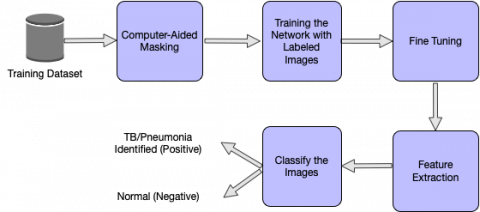
Segmentation is the partitioning of an image into various segments which are a set of pixels. It is based on the similarity of pixel components, the pixels which are similar are grouped into one cluster. It can be implemented using clustering, thresholding, edge-detection, etc. Thresholding is a very simple method that helps to create binary images from gray scale images. These conventional techniques give out lesser accuracy, in comparison to artificial neural networks, which has given scope for many novel approaches such as the usage of convolutional neural networks to perform image segmentation [13]. CNN produces heat maps or masks as outputs when an input image is given to it. Regions of high similarity among the adjacent pixels are formed shown in Figure 1. The network should be initially trained with a set of input images and their masks, and later heat maps or masks would be generated for the test images.
Figure 1. Phases of the proposed approach
In our proposed approach, we are using a convolutional neural network to segment the given chest radiographs (CXR) to detect pneumonia.
4.2 Dataset overview
We used a RSNA pneumonia dataset, which is divided into both, train and test image samples. The training labels that are provided tell the coordinates of the mask in the images. All the train images are in DICOM format. The train labels are provided with a set of patients and bounding boxes. The bounding boxes are defined as, x-min y-min width height. There is a binary target column Target, indicating Pneumonia or Non-Pneumonia and there may be multiple rows per Patient ID. There are 26,684 input CXRs and 3000 test CXRs. The train labels file comprises the filename, and the pneumonia locations which are transformed into a dictionary wherein the filename acts as the key and the pneumonia locations are the values. This dictionary only has file names where pneumonia is detected, and if there is no pneumonia in that file, it is not included in the dictionary. Out of 26,684 images, 6012 files have shown a positive sign regarding the presence of pneumonia.
Dataset generator: The dataset is broken down into random chunks to feed these set of images and masks into the model. Along with this, a few parameters, say, the batch size, image size, if the images are to be shuffled, etc. are also given to the model. The images are resized to 256×256 from the original 1024×1024 and the default batch size used is 32. These images or CXRs are then sent to the Convolutional Neural Network to train the model. Graphical user interface testing is done by using real time data collected from Third -I imaging of nearly 88 chest x-ray images.
4.3 Proposed architecture for segmentation
The Convolutional Neural Network is trained such that different parameter values are optimized to extract useful features from the given input CXRs. The bounding boxes are drawn around the predicted areas of pneumonia. The network is initially given the training images and labels. CNNs then extract low-level features followed by high-level features. The proposed CNN has residual blocks with down sampling and convolutions. An up-sampling layer is used at last to resize the image to the original shape.
4.3.1 Residual block
Residual block is just a stack of layers, wherein the output of the previous layer is connected to the output of new layers. This increases the accuracy of the model, by repeating a set of Convolutional-Batch-Normalization [14]-Activation layers. In this residual setting, it is not just passing the output of layer 1 to layer 2. Instead, it adds up the outputs of layer 1 to the outputs of layer 2 [15]. In a conventional set of layers, the output y will be f(x). y=f(x) But in a residual block, the output would be, y=f(x)+x.
4.3.2 Down-sampling
Down-sampling reduces the size of the input image similar to the pooling operation. In our paper, the inputs are passed to Batch Normalization-Activation-Convolutional-Max Pool layers to perform the down sampling operation. It is a crucial operation in extracting the features from the images. Batch normalization is a technique for training very deep neural networks that standardizes the inputs to a layer for each mini batch. This has an effect of stabilizing the learning process in drastically reducing a number of training epochs require to train network.
4.3.3 Up-sampling
Up-sampling layer brings back the resolution of the down sampled information. It restores the image to its original resolution using interpolation. After the features are extracted, we need to find the original image which is segmented to detect and depict if there is any abnormality in the chest X-rays. To accomplish this, we use an up-sampling layer.
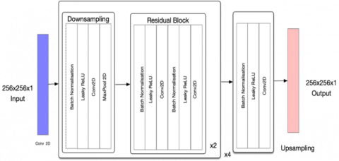
The proposed CNN architecture goes like this, the input image of size 256×256 is passed to the conv2d layer having 32 random filters with a size of 3×3, this gives 32 feature maps of size 256×256×1. Later, this image is down sampled using Batch-Normalization- Activation (Leaky ReLU) [16] Convolutional-Max Pool layers by a factor of 2 giving an image of size 128×128×64. To incorporate non-linearity, we are using Leaky ReLU. It solves the problem of vanishing gradients. The number of filters taken for every down sampling and the residual block is doubled, therefore, in the next pass, the number of filters would be 128. This helps in performing an in- depth analysis of the input image.
Next, this output is passed onto the residual blocks wherein Batch-Normalization, Leaky ReLU and convolutional operations are performed twice, adding the output to the input at last, which is the actual advantage of the residual block. We have taken 4 blocks performing down sampling operation, and for every down sampling operation, 2 residual blocks are created. After, a set of the above operations are performed, it down samples until the image diminishes to 16×16. To get the image back to the original size, an up-sampling operation is done which gives the output of image size 256×256. Layer-wise architecture is presented in the in Figure 2 and a detailed explanation of each layer given in Table 1.
Figure 2. Architecture of the proposed CNN
4.3.4 IoU or Jaccard loss function
Intersection over Union metric, also called as the Jaccard Index is a method to quantify the overlap between the target image and the predicted output. It is equal to the number of pixels common between these two images divided by the total number of pixels present across both of them.
$I o U=\frac{\text { target } \cap \text { prediction }}{\text { target } U \text { prediction }}$ (6)
The IoU is calculated over each class separately and then averaged over all classes to provide a global, mean IoU score.
4.3.5 BCE loss
BCE is the binary cross entropy which we typically use in a binary classification problem. In our paper, we are detecting if the person has pneumonia or not. Therefore, there are two classes to be dealt with. BCE can be defined as:
$B C E=-\sum_{i=1}^2\left(y_i \log (\hat{y}(i))\right)+\left(1-y_i\right) \log (1-\hat{y}(i))$ (7)
where, y is the given label and yˆ(i) is the observed label.
These two losses are combined to account for the total loss (IoU BCE loss) incurred in the network and mean IoU would be used as a metric to compile the model.
4.3.6 Cosine annealing
Cosine annealing can be alternatively called as Stochastic Gradient Descent with Restarts [17]. It decreases the learning rate in the form of half a cosine curve. This is useful because at first, we can start out with higher learning rates and later decrease as we get closer to the local minimum, which assist the network to go very deeply and to know what is actually happening when the network is under training, and is a successful parameter in the neural network in real-world systems. This helps in exploring the deeper, but narrower parts of the loss function and has shown good results in comparison to the case where the learning rate is constant. We have used this formula for updating the learning rate:
$l r=\operatorname{lr} * \frac{(\cos (\pi * x / \text { epochs })+1)}{2}$ (8)
$\pi * x /$ epochs restricts the cosine range from -1 to 1. 1 is added to it which gives the range varying from 0 to 2. Now, this is divided by 2 which halves it to revert it back to 0 to 1. This way, the learning rate decreases from the max value and then again restarts with the maximum at the beginning of the next cycle.
A neural network model entirely relies on the metrics that we consider for the training. In literature, we have seen many training models which are used for the segmentation process. Few architectures like LeNet [18], ResNet [15], AlexNet [19], and ChexNet [20] have many layers which take much time for training on a standard CPU. However, training a neural network with thousands of images takes more than days over a CPU, hence we trained our network on a cloud-based GPU. The hardware specifications include 12GB of NVIDIA TESLA RAM and 8 Cores of CPU. To speed up the training process, the input will be given in batches from the training set.
Table 1. Layers in the proposed CNN architecture
|
Layer |
Type |
Input Size |
Output Size |
No. of Filters |
Filter Size |
|
Layer 1 |
Conv |
256×256×1 |
256×256×32 |
32 |
3x3 |
|
Layer 2-5 |
Batch+Leaky+Conv+MaxPool |
256×256×32 |
128×128×64 |
64 |
1x1 |
|
Layer 6-17 |
(Batch+Leaky+Conv)x4 |
128×128×64 |
128×128×64 |
64 |
3x3 |
|
Layer 18-21 |
Batch+Leaky+Conv+MaxPool |
128×128×64 |
64×64×128 |
1128 |
1x1 |
|
Layer 22-33 |
(Batch+Leaky+Conv)x4 |
128×128×64 |
64×64×128 |
128 |
3x3 |
|
Layer 34-37 |
Batch+Leaky+Conv+MaxPool |
64×64×128 |
32×32×256 |
256 |
1x1 |
|
Layer 38-49 |
(Batch+Leaky+Conv)x4 |
32×32×256 |
32×32×256 |
256 |
3x3 |
|
Layer 50-53 |
Batch+Leaky+Conv+MaxPool |
32×32×256 |
16×16×512 |
512 |
1x1 |
|
Layer 54-65 |
(Batch+Leaky+Conv)x4 |
16×16×512 |
16×16×512 |
512 |
3x3 |
|
Layer 66-68 |
Batch+Leaky+Conv |
16×16×512 |
16×16×1 |
1 |
1x1 |
|
Layer 69 |
Upsampling |
16×16×1 |
256×256×1 |
- |
- |
|
Layer 70 |
Unsampling |
16×16×1 |
256×256×1 |
- |
- |
Training the network includes three main steps. Initially, the images are loaded from the training dataset and preprocessed based on the input dimensions of the network. Here the images are resized to the aspects of 256×256×1, and the networks’ first layer has the same number of neurons. Second, we need to segment the pathologies affected regions of the lungs where we will be using convolutions and pooling layers. This feature extraction is achieved by training the network with input images and the masked areas from the CSV files. Lastly, the network is qualified to be a classifier. To this, labels are provided to the CXR images as vectors which contain value 1 for the pneumonia (positive class) and 0 for the non-pneumonia case.
The proposed network is a 69 layers convolutional architecture, taken as an inspiration from u-net architecture. A sequence of layers, namely convolutions, batch normalization, and up sampling layers are arranged in the intended network for feature extraction. LeakyRelU incorporates the removal of linearity between the layers by adjusting the weights of the net- work. This architecture is trained over 25 epochs, and an epoch is defined as one complete forward pass and backward pass. The weights get updated in the forward pass and updated in the backward pass based on the given loss function.
69 layers are used to get accurate result, it gets out fitted if more than 69 layers are used, it gets under fitted if less than 69 layers are used. We use IOU BCE loss and Adam optimizer as the parameters and both, train and validation sets are obtained using the dataset generator described in the dataset section.
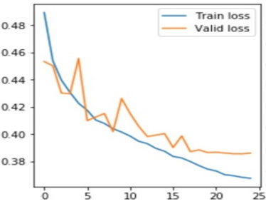
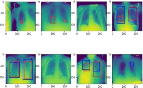
The results are evaluated based on the performance of the network on the test dataset. The test dataset is generated using the dataset generator with a batch size of 25 and images resized to 256×256. As discussed in the previous section, the original dataset is divided into two parts, one for training and one for validation. Out of the 26,684 images, 6012 are considered for validation purposes. The model is given a set of 3000 CXR images to segment and identify the pathologies, in this case for Pneumonia. The labeled dataset consists of 1001 images of pneumonia masked images. Main metrics used to evaluate the model are the accuracy, loss and IoU for the network. Accuracy is defined as the ratio of correctly predicted pneumonia images on the dataset to the total number of pneumonia-identified-images. Before the training, all the weights of the network are initiated to zero mean, biases are randomly initialized in the range -1 to 1 with a standard deviation of 0.001. The train and validation losses have decreased remarkably, from 0.49 to 0.39 and 0.45 to 0.41 respectively. The model could successfully achieve 97.4% accuracy on the trained dataset, 97.2% accuracy on the validation set, and 90.2% accuracy on the test dataset shows in Figure 3. The train and validation IoU increased throughout, reaching values of 0.74 and 0.72 respectively. Validation accuracy, validation loss, and validation intersection over union (IoU) values are compared throughout the whole training process which is represented visually below Figure 4 and Figure 5. If pneumonia is detected, bounding boxes are drawn around the detected areas in the CXRs. Below are the results and the experiments that are obtained after the training Figure 6.
Figure 3. Graph depicting the train and validation accuracy
Figure 4. Graph depicting the train and validation loss
Figure 5. Graph depicting the train and validation IoU
Figure 6. Bounding boxes drawn for the test images obtained using the parameters from the trained model
In our paper, we have proposed a CNN architecture for the detection of pneumonia, this can be generalized to Tuberculosis. Now, instead of resorting to manual techniques for finding out the presence of lung abnormalities, we put forth an easier and reliable way to automatically detect pneumonia. This is the need of the hour which could be used in areas where people are more prone to Pneumonia/Tuberculosis. The complexity of the proposed technique is high when dealing with bigger datasets. This work in the context of global pandemic (Covid19), can be used a very good aid by the doctors to analyse the patients condition and to better the process of diagnose in quick time.
The authors thank to Koneru Lakshmaiah Educational Foundation, Vijayawada, for his providing characterization supports to complete research work.
[1] Bhutia, R., Narain, K., Devi, K.R., Singh, T.S.K., Mahanta, J. (2013). Direct and early detection of Mycobacterium tuberculosis complex and rifampicin resistance from sputum smears. The International Journal of Tuberculosis and Lung Disease, 17(2): 258-261. https://doi.org/10.5588/ijtld.12.0452
[2] Priya, E., Srinivasan, S. (2016). Automated object and image level classification of TB images using support vector neural network classifier. Biocybernetics and Biomedical Engineering, 36(4): 670-678. https://doi.org/10.1016/j.bbe.2016.06.008
[3] Van Ginneken, B., Katsuragawa, S., ter Haar Romeny, B. M., Doi, K., Viergever, M.A. (2002). Automatic detection of abnormalities in chest radiographs using local texture analysis. IEEE Transactions on Medical Imaging, 21(2): 139-149. https://doi.org/10.1109/42.993132
[4] Horváth, G., Orbán, G., Horváth, Á., Simkó, G., Pataki, B., Máday, P., Juhász, S. (2009). A cad system for screening x-ray chest radiography. In World Congress on Medical Physics and Biomedical Engineering, September 7-12, 2009, Munich, Germany, pp. 210-213. https://doi.org/10.1007/978-3-642-03904-1_59
[5] Guo, G., Wang, H., Bell, D., Bi, Y., Greer, K. (2003). KNN model-based approach in classification. In OTM Confederated International Conferences "On the Move to Meaningful Internet Systems", pp. 986-996. https://doi.org/10.1007/978-3-540-39964-3_62
[6] Hogeweg, L., Mol, C., Jong, P.A.D., Dawson, R., Ayles, H., Ginneken, B.V. (2010). Fusion of local and global detection systems to detect tuberculosis in chest radiographs. In International Conference on Medical Image Computing and Computer-Assisted Intervention, pp. 650-657. https://doi.org/10.1007/978-3-642-15711-0_81
[7] Jaeger, S., Karargyris, A., Antani, S., Thoma, G. (2012). Detecting tuberculosis in radiographs using combined lung masks. In 2012 Annual International Conference of the IEEE Engineering in Medicine and Biology Society, San Diego, CA, USA, pp. 4978-4981. https://doi.org/10.1109/EMBC.2012.6347110
[8] Karargyris, A., Siegelman, J., Tzortzis, D., Jaeger, S., Candemir, S., Xue, Z., Santosh, K.C., Vajda, S., Antani, S., Folio, L., Thoma, G.R. (2016). Combination of texture and shape features to detect pulmonary abnormalities in digital chest X-rays. International Journal of Computer Assisted Radiology and Surgery, 11(1): 99-106. https://doi.org/10.1007/s11548-015-1242-x
[9] Maduskar, P., Philipsen, R.H., Melendez, J., et al. (2016). Automatic detection of pleural effusion in chest radiographs. Medical Image Analysis, 28: 22-32. https://doi.org/10.1016/j.media.2015.09.004
[10] O'Shea, K., Nash, R. (2015). An introduction to convolutional neural networks. arXiv preprint arXiv:1511.08458. https://arxiv.org/abs/1511.08458
[11] Koushik, J. (2016). Understanding convolutional neural networks. arXiv preprint arXiv:1605.09081.
[12] Srivastava, N., Hinton, G., Krizhevsky, A., Sutskever, I., Salakhutdinov, R. (2014). Dropout: a simple way to prevent neural networks from overfitting. The Journal of Machine Learning Research, 15(1): 1929-1958.
[13] Kurama, V., Alla, S., Rohith, V.K. (2018). Image semantic segmentation using deep learning. International Journal of Image, Graphics and Signal Processing, 10(12): 1-1. https://doi.org/10.5815/ijigsp.2018.12.01
[14] Ioffe, S., Szegedy, C. (2015). Batch normalization: Accelerating deep network training by reducing internal covariate shift. In International Conference on Machine Learning, pp. 448-456.
[15] He, K., Zhang, X., Ren, S., Sun, J. (2016). Deep residual learning for image recognition. In Proceedings of the IEEE Conference on Computer Vision and Pattern Recognition, pp. 770-778. https://doi.org/10.1109/CVPR.2016.90
[16] Ramachandran, P., Zoph, B., Le, Q.V. (2017). Searching for activation functions. arXiv preprint arXiv:1710.05941. https://arxiv.org/abs/1710.05941
[17] Loshchilov, I., Hutter, F. (2016). SGDR: Stochastic gradient descent with warm restarts. arXiv preprint arXiv:1608.03983. https://arxiv.org/abs/1608.03983
[18] Krizhevsky, A., Hinton, G. (2009). Learning multiple layers of features from tiny images.
[19] Krizhevsky, A., Sutskever, I., Hinton, G.E. (2017). Imagenet classification with deep convolutional neural networks. Communications of the ACM, 60(6): 84-90. https://doi.org/10.1145/3065386
[20][1] Bhutia, R., Narain, K., Devi, K.R., Singh, T.S.K., Mahanta, J. (2013). Direct and early detection of Mycobacterium tuberculosis complex and rifampicin resistance from sputum smears. The International Journal of Tuberculosis and Lung Disease, 17(2): 258-261. https://doi.org/10.5588/ijtld.12.0452
[2] Priya, E., Srinivasan, S. (2016). Automated object and image level classification of TB images using support vector neural network classifier. Biocybernetics and Biomedical Engineering, 36(4): 670-678. https://doi.org/10.1016/j.bbe.2016.06.008
[3] Van Ginneken, B., Katsuragawa, S., ter Haar Romeny, B. M., Doi, K., Viergever, M.A. (2002). Automatic detection of abnormalities in chest radiographs using local texture analysis. IEEE Transactions on Medical Imaging, 21(2): 139-149. https://doi.org/10.1109/42.993132
[4] Horváth, G., Orbán, G., Horváth, Á., Simkó, G., Pataki, B., Máday, P., Juhász, S. (2009). A cad system for screening x-ray chest radiography. In World Congress on Medical Physics and Biomedical Engineering, September 7-12, 2009, Munich, Germany, pp. 210-213. https://doi.org/10.1007/978-3-642-03904-1_59
[5] Guo, G., Wang, H., Bell, D., Bi, Y., Greer, K. (2003). KNN model-based approach in classification. In OTM Confederated International Conferences "On the Move to Meaningful Internet Systems", pp. 986-996. https://doi.org/10.1007/978-3-540-39964-3_62
[6] Hogeweg, L., Mol, C., Jong, P.A.D., Dawson, R., Ayles, H., Ginneken, B.V. (2010). Fusion of local and global detection systems to detect tuberculosis in chest radiographs. In International Conference on Medical Image Computing and Computer-Assisted Intervention, pp. 650-657. https://doi.org/10.1007/978-3-642-15711-0_81
[7] Jaeger, S., Karargyris, A., Antani, S., Thoma, G. (2012). Detecting tuberculosis in radiographs using combined lung masks. In 2012 Annual International Conference of the IEEE Engineering in Medicine and Biology Society, San Diego, CA, USA, pp. 4978-4981. https://doi.org/10.1109/EMBC.2012.6347110
[8] Karargyris, A., Siegelman, J., Tzortzis, D., Jaeger, S., Candemir, S., Xue, Z., Santosh, K.C., Vajda, S., Antani, S., Folio, L., Thoma, G.R. (2016). Combination of texture and shape features to detect pulmonary abnormalities in digital chest X-rays. International Journal of Computer Assisted Radiology and Surgery, 11(1): 99-106. https://doi.org/10.1007/s11548-015-1242-x
[9] Maduskar, P., Philipsen, R.H., Melendez, J., et al. (2016). Automatic detection of pleural effusion in chest radiographs. Medical Image Analysis, 28: 22-32. https://doi.org/10.1016/j.media.2015.09.004
[10] O'Shea, K., Nash, R. (2015). An introduction to convolutional neural networks. arXiv preprint arXiv:1511.08458. https://arxiv.org/abs/1511.08458
[11] Koushik, J. (2016). Understanding convolutional neural networks. arXiv preprint arXiv:1605.09081.
[12] Srivastava, N., Hinton, G., Krizhevsky, A., Sutskever, I., Salakhutdinov, R. (2014). Dropout: a simple way to prevent neural networks from overfitting. The Journal of Machine Learning Research, 15(1): 1929-1958.
[13] Kurama, V., Alla, S., Rohith, V.K. (2018). Image semantic segmentation using deep learning. International Journal of Image, Graphics and Signal Processing, 10(12): 1-1. https://doi.org/10.5815/ijigsp.2018.12.01
[14] Ioffe, S., Szegedy, C. (2015). Batch normalization: Accelerating deep network training by reducing internal covariate shift. In International Conference on Machine Learning, pp. 448-456.
[15] He, K., Zhang, X., Ren, S., Sun, J. (2016). Deep residual learning for image recognition. In Proceedings of the IEEE Conference on Computer Vision and Pattern Recognition, pp. 770-778. https://doi.org/10.1109/CVPR.2016.90
[16] Ramachandran, P., Zoph, B., Le, Q.V. (2017). Searching for activation functions. arXiv preprint arXiv:1710.05941. https://arxiv.org/abs/1710.05941
[17] Loshchilov, I., Hutter, F. (2016). SGDR: Stochastic gradient descent with warm restarts. arXiv preprint arXiv:1608.03983. https://arxiv.org/abs/1608.03983
[18] Krizhevsky, A., Hinton, G. (2009). Learning multiple layers of features from tiny images.
[19] Krizhevsky, A., Sutskever, I., Hinton, G.E. (2017). Imagenet classification with deep convolutional neural networks. Communications of the ACM, 60(6): 84-90. https://doi.org/10.1145/3065386
[20] Rajpurkar, P., Irvin, J., Zhu, K., Yang, B., Mehta, H., Duan, T., Ding, D., Bagul, A., Langlotz, C., Shpanskaya, K., Lungren, M.P., Ng, A.Y. (2017). Chexnet: Radiologist-level pneumonia detection on chest x-rays with deep learning. arXiv preprint arXiv:1711.05225. https://arxiv.org/abs/1711.05225