An Industrial Application Towards Classification and Optimization of Multi-Class Tile Surface Defects Based on Geometric and Wavelet Features

2.1 Machine vision environment

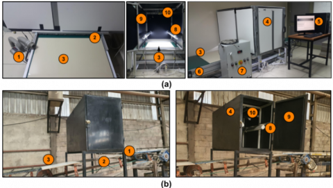
To obtain tile images, a machine vision environment consisting of a lighting cabinet, camera, conveyor belt, and imaging computer has been created at the laboratory and also at the factory production line of Usak Seramik. The image of the machine vision environments is given in Figure 1. An attempt was made to simulate a factory production line in the machine vision environment. Figure 1(a) is the image processing infrastructure implemented in the experimental environment. Figure 1(b) is the prototype created for the factory environment.

1.png

Figure 1. Experimental (a) and industrial (b) machine vision environment for tile inspection

First of all, when a ceramic tile comes in line with the cabinet on the production line, the brush (2) and the air blasting machine (1) start to work. Thus, it clears the tile surface from dusts. If dusts remain on the ceramic tiles surface, the system will act as a defect, causing problems with surface quality and defect classification. At this stage, thanks to the illumination light, it provides an ideal environment that focus to attributes of the image and ensures that it is distributed homogeneously. Homogeneous distribution of light is provided on the surface of the ceramic tile, thanks to the luminaire lens and the diffuser. In this study, LED lights were preferred due to their low power consumption and small footprint. For homogeneous lighting, two linear lighting rods (8) are used at opposite angles to the surface. The green (6) conveyor belt provides controllable movement at the factory's production line speed. This speed can be changed with the speed control device (7) to test different production speeds. Thus, as the ceramic tiles (3) are inside the lighting cabinet (4), the video images of the ceramic tile are captured by the line camera (10) and sent to the software system (5) in a simple way. The inner surface of the lighting cabinet (9) is covered with matte black material to prevent reflections that may occur due to lighting. The computer in the imaging system (5) has an Intel Core i7-9750H CPU with 24GB of RAM and 12MB of cache. The graphics card is NVIDIA GeForce GTX 1050 4GB and 640 cores. Basler brand line scan camera with 51 kHz over GigaE, 2k resolution and a global shutter is used to capture the images.

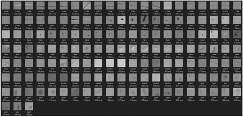
The training data set of the system consists of five different defect classes: point, scratch, pore, speckle and crack. Each tile surface may have a different number and type of surface defects. 30 images were generated for crack defects. In order to create a balanced data set in the laboratory environment, 30 different defect images of each defect type (150) in 64×64 dimensions were used. Example defect images of the data set used in the study are given in Figure 2.

2.png

Figure 2. Defect images data set [12]

2.2 Filtering & binarization

The Steerable Digital Filter (SDF) acts like a Gabor filter because it has a directional structure. SDF was presented by Freeman and Adelson [13] in 1991. It has various applications in image processing such as texture analysis, enhancement and edge detection. In the filtering process, input data is passed through basic filters with different orientations and then subdivided to find the orientation properties. No matter what angle value of the directional filter is specified, after an image is passed through a steerable filter, the edges of that angle dominate the image, while at certain angle values, the directions away from this angle weaken or disappear completely. In order to realize this filter, the first derivative of the two-dimensional Gaussian function in Eq. (1) is applied as a steerable filter [14].

$g(x, y)=e^{-\left(x^2+y^2\right) / 2}$             (1)

Gaussian functions are often used to represent the probability density function of a normally distributed random variable. The normalizing constant or scaling constant is used to reduce any probability function to a probability density function with total probability of one. Since a directed filter will be applied on an image here, a probability density function with a total probability of 1 is not needed. Besides, the normalization constant is utilized for univariate Gaussians. Therefore, scaling constant can be ignored [15-17]. For this reason, the scaling constant $1/\sqrt{2} \pi$ is not taken into account in Eq. (1) for a simpler structure. A simpler example of a steerable function is presented in Eq. (2).

$g_x(x, y)=\frac{\partial g(x, y)}{\partial x}=-x e^{-\left(x^2+y^2\right) / 2}$             (2)

The orientable function can be represented with Eq. (3) in polar coordinates.

$g_x(r, \theta)=-r e^{-r^2 / 2} \cos \theta$                (3)

The expression given above results from an angular component and a radial component corresponding to a polar separable function. For example, it can be given as in Eq. (4), giving $\alpha=\pi / 2$ rotation [13].

$g_x\left(r, \theta-\frac{\pi}{2}\right)=-r e^{-r^2 / 2} \cos \left(\theta-\frac{\pi}{2}\right)=-r e^{-r^2 / 2} \sin (\theta)$            (4)

In fact, if the steerable function is returned to any angle α, the result can be given as Eq. (5).

$g_\alpha(r, \theta-\alpha)=\cos (\alpha) g_x+\sin (\alpha) g_y$            (5)

where, g_x and g_y denote horizontally and vertically oriented derivatives in Eq. (5), respectively. To use the SDF on an image, the orientation properties of the input image must be revealed. The image used as input is first passed through basic filters with different orientations and then subdivided. For this reason, a filter function with a rotatable structure in Eq. (6) can be given as a linear sum of its rotated versions.

$g_\alpha(x, y)=\sum_{i=1}^M k_j(\alpha) g_{\alpha j}(x, y)$           (6)

The resulting image consists of certain directional impact responses for the system defined at a certain angle in the α value and the weighted sum of g_αj(x, y) in the α direction. k_j(α) are the weight coefficients and provide control of the filter orientation in the α direction.

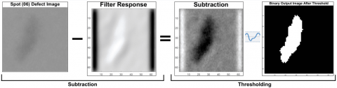
For the SDF filter, the directed filter responses of the defect images are processed as a filter output image. Pixel values indicating edges in different directions and in the same direction are converted to binary images in binaryization with the image used as output. First, the filter output matrix is subtracted numerically from the grayscale defect images matrix. The average values of the filter output image are then obtained as a one-dimensional array. Then the average value of the average one-dimensional array is calculated. Pixel values greater than the threshold value in the faulty image sequence are obtained from binary output images. In this way, the adaptive thresholding method is realized. Binarization process is given in Figure 3.

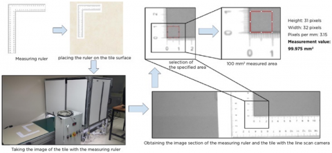
In line scanning cameras, resolution and image transfer rate are calculated according to the speed of the moving object, unlike area scanning cameras. In this context, the required transmission rate and camera line frequency rate to obtain tile images were calculated. By using the desired image width (W), the number of pixels per mm (ppm) and the conveyor belt speed (S), the image size to be transferred per second from the line scan camera was calculated in MB/s. The number of pixels corresponding to the real area of 100 mm² on the image were measured horizontally and vertically using the ImageJ program. By taking the average of these values, the average pixel number (ppm) corresponding to 1 mm was calculated. The measurement steps are given in Figure 4. The 100 mm² area width was measured as 32 pixels and the height as 31 pixels by the camera. The mean ppm value was calculated as 3.15 and measured as 100 mm², 99.975 mm², and 992 pixels. The relative error was found to be 0.00025. Since the relative error is quite small, it is considered negligible.

3.png

Figure 3. Binarization process

4.png

Figure 4. Calculation of the average number of pixels for 1mm

5.png

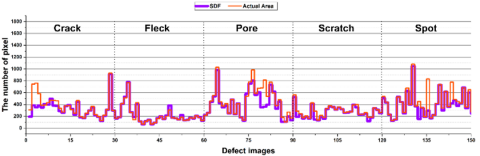
Figure 5. Number of defect area pixels calculated after filtering

6.png

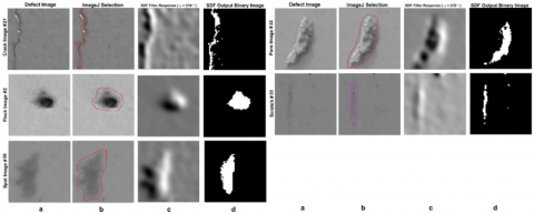
Figure 6. Results of filtering and binarization, (a) The raw surface defect image, (b) The actual defect area pixels in ImageJ program, (c) SDF filter response, (f) SDF output binary image

7.png

Figure 7. Segmentation and feature extraction process

The ability to represent real defect areas of binary images is demonstrated by comparing the pixel counts of the real defect areas with the pixel counts of the binary images. The number of pixels formed in the output images is counted after binaryization. The actual area pixel number is calculated manually by the ceramic engineers at Uşak Seramik via the ImageJ program and is accepted as a reference value. SDF filtering images of the randomly selected error image from the error classes, binary images, and the actual error area selection obtained using ImageJ are given in Figure 5.

The number of defect area pixels of the defect images in the dataset was found and given in Figure 6. It was observed that the number of defective area pixels calculated using the SDF matched the actual number of defective areas in Figure 6.

2.3 Feature extraction

Geometric Feature: Before debugging the features of the errors, the image areas of the errors in the filtered and preprocessed tile image segment should be segmented. Black vertical lines and horizontal lines in the section image are removed for segmentation. The remaining white areas are defined as defective areas. To calculate the geometric features, specific features of the defect must be determined. Geometric features were determined from the pixel value positions (coordinates) on the binary defect image. The segmentation and feature extraction process of the defect images on the sample tile image section containing the spot defect in the software environment is given in Figure 7.

Explanations of the geometrical properties specified in Figure 6 are given in Table 1. The h is explained as the height of the smallest rectangle surrounding the defect and calculated as the number of pixels along the defect length. The w is explained as the width of the smallest rectangle surrounding the defect and calculated as the number of pixels across the width of the defect.

Table 1. Geometric properties of defect

Table 2. Geometric features of defect

8.png

Figure 8. Vertical, horizontal and diagonal detail coefficients of sample defect images

The geometric features are given in Table 2 were calculated by using the geometric properties specified in Figure 7 and Table 1.

Wavelet Features: The wavelet transform method is used to extract the frequency domain features of the defect images. Wavelet transform is a feature extraction tool that divides data, functions, or operators into different frequency components and then examines each component with a resolution appropriate to its scale [18]. The wavelet transform uses narrower windows as window length at high frequencies, while wider windows are used at low frequencies. Therefore, it is useful in the frequency domain when converting a signal or image into lower-dimensional data that can be represented. For this purpose, a single-level 2-dimensional (2-D) Haar-type discrete wavelet transform was used for images. First, a 1-D filter bank was applied to the rows of the image. Then, the same transformation is applied to the columns of each channel of the result. For this reason, 3 high-pass channels (detail coefficient) corresponding to vertical, horizontal, and diagonal and one approach image were obtained. The resulting surface view map of the vertical, horizontal, and diagonal 1st level detail coefficients is presented in Figure 8. The averages of the obtained wavelet coefficients were calculated and evaluated as the feature value. The mean, variance, and standard deviations of the obtained wavelet coefficients were calculated, respectively. These values are evaluated as the feature value. The best accuracy result has been obtained through diagonal coefficients.

2.4 SVM classification

As a machine learning algorithm, the SVM based on supervised learning, which is used as a fast classifier in the literature, was used. In simple terms, SVM can be defined as the separation of the data of two different classes on the same plane, with a boundary line formed by a linear equation. SVM is a kernel-based learning approach that gives very fast and accurate results in subjects such as linear and nonlinear classification, regression analysis, outlier detection, function, and density estimation. It is especially used in classification problems where the patterns between the variables of the data to be classified in data mining are not known. Real-life classification problems are often non-linear problems made up of many different classes. SVM aims to solve these problems more easily by making the nonlinear sample space linear on a higher plane. While doing this, it tries to find the linear equation that maximizes the distance between the closest elements of the classes. This is called margin maximization in the literature [19-23]. In other words, SVM aims to create the furthest upper (hyper) plane between the vectors of two classes with a linear decision function. The positive aspects of SVM can be listed as follows;

• It does not require prior knowledge assumption about the distribution.

• It achieves high accuracy values.

• Model complex decision boundaries.

• It can work with a large number of independent variables.

• It can work with both linear and non-linearly separable data.

• Compared to other classification methods, the problem of overfitting is less.

The SVM method is widely used in two-class problems [24].

Within the scope of the study, the data processed in SVM were used linearly. The problem that is tried to be solved in this paper is accepted as a multiple classification problem because it consists of 5 classes. SVM is insufficient as it stands. For this reason, for each class belonging to the surface defect classes, it was tried to be solved as a binary classification problem by accepting all other classes as a single class. It has been accepted as the one against all (one vs. all) method in the literature. Two feature types should be used in the solution of binary classification problems. Since the best results from these features were obtained from F1 and F2 features. These features were used for classification. Of the 150 feature values, 90 data (60%) were used for training and 60 data (40%) for test. Polynomial and RBF are used as SVM kernel functions. The Sequential Minimum Optimization (SMO) method was chosen as the optimization solver in the SVM model. In the studies conducted with the SVM algorithm, the effect of different kernel functions on classification success was investigated. In some studies, the RBF kernel function-based classifier was found to be more successful, and in some studies, the polynomial kernel-function classifier was more successful [25-30]. Therefore, in this study, the success of both core functions in classification was measured.

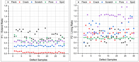
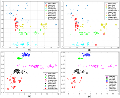
The classification was carried out by selecting the F₁- Extend ratio and F₂- Lining ratio feature groups using the SVM method. F₁ and F₂ features data graphics are given in Figure 9.

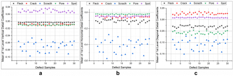
1st level wavelet detail coefficients of vertical, horizontal, and diagonal are given in Figure 10 respectively.

Classification results of geometric and wavelet feature with different kernel functions (RBF, polynomial) are given in Figure 11a, Figure 11b, Figure 11c, and Figure 11d respectively.

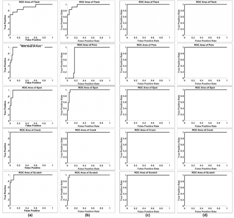
ROC (Receiver Operator Characteristic) graphics of each defect class of geometric features with different kernel functions (RBF, polynomial) are given in Figure 12a and Figure 12b respectively. ROC (Receiver Operator Characteristic) graphics of each defect class of wavelet features with different kernel functions (RBF, polynomial) are given in Figure 12c and Figure 12d respectively.

The confusion matrix of each class of geometric and wavelet features with RBF and polynomial kernel function are given in Figure 13a, Figure 13b, Figure 13c, and Figure 13d respectively. The classification performance results obtained using the confusion matrix are given in Table 5.

When Table 5 is examined, it is seen that 100% classification success is achieved for all classes and all core functions with wavelet features. It is seen that a higher success value is obtained compared to the results obtained in the previous study [30] and manual examination. Also, it seems that kernel functions do not have a direct effect on classification success. The validation losses for the cross-validation classification model of the classification model obtained using the SVM method are given in Table 6.

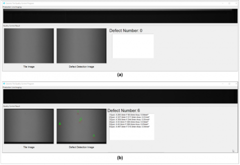
It can be seen that the validation loss is quite low for the attributes and kernel functions of all classes from Table 6. This result shows that correct results are produced for classification with SVM in all feature groups. Although it is understood that there is no effect of kernel functions in the classification results given in Figure 12c, Figure 12d, Figure 13c, Figure 13-d, and Table 5 for the wavelet feature group, when the validation loss values given in Table 6 are examined, it is more difficult because the validation loss of the radial basis kernel function is small when the data set grows. It is expected to produce successful results. The real-time application interface of detection system is given in Figure 14. The localizations of the defects are also determined in real-time application. The application software is developed in Python language. It is planned to run on operating systems such as Windows, Ubuntu. Also, it can run computers such as Raspberry Pi or Nvidia Jetson tx2. The developed system was set up for testing at the Uşak Seramik factory. The industrial machine vision environment is given in Figure 15.

9.png

Figure 9. F₁ and F₂ feature set

10.png

Figure 10. 1st level wavelet detail coefficient means, (a) vertical, (b) horizontal, (c) diagonal

11.png

Figure 11. Classification results

12.png

Figure 12. ROC area of each class

13.png

Figure 13. Confusion matrix of each class

Table 5. Classification results

Table 6. Validation loss for the cross-validation classification model of classes with the SVM

14.png

Figure 14. Real-time application interface

15.jpg

Figure 15. Test phase of industrial machine vision environment