Bhavya Kanchanapalli* | Rama Rao Pokanati Veera Vekata | Ravi Srinivas Lanka
© 2022 IIETA. This article is published by IIETA and is licensed under the CC BY 4.0 license (http://creativecommons.org/licenses/by/4.0/).
OPEN ACCESS
The Interline Power Flow Controller (IPFC) is a voltage source converter based Flexible AC Transmission System (FACTS) controller for series compensation and power flow management among a substation's multiline transmission systems. Individual Voltage Source Converters (VSC) can inject reactive voltage that can be adjusted to manage active power flow in a line. This VSC is used to convert DC voltage to AC voltage and the voltage is kept constant in the entire process. In this article, a circuit model for IPFC is constructed, and a simulation of an interline power flow controller is performed, with control performed utilizing a variety of algorithms, including adaptive weighted feedback, gravitational search, BAT, and ANT colony optimization. The system's performance was evaluated in a variety of scenarios, including fault incidence, synchronous load connection, and asynchronous load connection. The design of system and analysis of system has been carried out using MATLAB Simulink in terms of various parameters at point of common coupling like voltage, current, power and power factor.
interline power flow controller, adaptive weighted feedback algorithm, gravitational search, BAT, and ANT colony optimization
Energy is delivered to loads that fulfil a purpose through power systems. These loads include everything from household items to heavy machines. Most loads demand a specific voltage, as well as a specific frequency and number of phases for alternating current devices. Single-phase equipment in your house, for example, will generally operate at 50 or 60 Hz with a voltage ranging from 110 to 260 volts (depending on national standards). The exception is centralized air conditioning systems, which are now almost always three-phase in order to function more effectively. Wattage is a measurement of how much electricity a gadget consumes and is found on all devices in your home. The net [1] quantity of power used by loads on a power system at any given moment must match the net amount of power provided by suppliers less the power lost in transmission.
One of the most difficult aspects of power system engineering is ensuring that the voltage, frequency, and amount of power delivered to the loads meet expectations. However, it is not the only issue; in addition to the power consumed by a load to perform meaningful work (known as actual power), many alternating current devices [2-4] consume additional power as a result of the alternating voltage and alternating current becoming slightly out of sync (termed reactive power). Reactive power, like actual power, must balance (that is, the reactive power generated on a system must equal the reactive power used) and can be supplied by generators, though capacitors are generally more cost-effective (see "Capacitors and reactors" below for more details). A final point to consider when it comes to loads is power quality. A variety of temporal difficulties can negatively impact power system loads, in addition to persistent over voltages and under voltages (voltage regulation issues) and sustained departures from the system frequency (frequency regulation issues). Voltage sags, dips, and swells, transient over voltages, flicker, high frequency noise, phase mismatch, and low power factor are all examples of these issues. When the power supply to a load deviate from the ideal, power quality concerns arise: The ideal current and voltage fluctuation as a perfect sine wave at a given frequency with the voltage at a defined amplitude for an AC supply. The optimal voltage for a DC supply is one that does not change from a set level. When it comes to specialized industrial gear or medical equipment, power quality is extremely crucial.
The power transfer capability of traditional AC [5] transmission has been limited by numerous dynamic and static constraints such as transient stability, voltage stability, thermal limits, and so on. Because of these intrinsic power system limitations, current transmission sources have been underutilized. Fixed and mechanically switched series and shunt capacitors, reactors, and synchronous generators are used in traditional techniques to solve these difficulties. However, due to sluggish response times and mechanical component wear and tear, the necessary response has not been achieved. The creation of thyristor devices led to the development of power electronic converters, which led to the implementation of FACTS controllers [6]. These power electronic-based controllers can offer power system control that is smooth, continuous, fast, and repeatable. The term FACTS stands for Flexible AC Transmission System, and it refers to the use of power electronic devices in electrical transmission systems. It's an AC transmission system with a power electronic controller and additional static controllers to help with control and power transfer. It enhances electrical network performance by balancing active and reactive power.
Typical devices in the first-generation period include tap changing and phase changing transformers, synchronous generators, and series capacitors. Other from series capacitors, which are sometimes known as capacitor banks, the rest of the devices are dynamic. The majority of these devices are operated on the generating side of the power grid, and they are generally costly. When it comes to series capacitors, the disadvantage of this device cannot be overlooked. Because the device is made up of numerous fixed-capacitance capacitors, it is difficult to regulate in order to provide the grid with the true not-fixed capacitance.
The FACTs devices of the second generation are divided into two categories: thyristor-based devices and fully-controlled devices-based compensators. The thyristor is known as a half-controlled device [7-9] since it can only be switched on but not off. This category includes Static Var Compensator (SVC) and Thyristor-Controlled Series Capacitor (TCSC). GTO and other completely regulated devices are the most common. This category includes the Static Compensator (STATCOM), the Solid State Series Compensator (SSSC), the Unified Power Flow Controller (UPFC), and the HVDC-Voltage Source Converter (HVDC-VSC). In most nations and continents, AC transmission lines are the backbone of the electrical system. Unless active grid elements are utilized, the power flow will follow the path of least impedance and will be uncontrolled. Flexible ac transmission systems (FACTS) use power electronics to improve the operation of the ac transmission grid. The transmission system operator has some control over these devices.
The Interline Power Flow Controller (IPFC) is a static synchronous series compensator that has been extended. The IPFC appeared as a standoff solution for the power flow management of multiline systems, replacing separately managed UPFC (unified power flow controller) in each line, because to the high cost of high power semiconductors and convertors dropping gradually. The proposed work analyzed the performance of the Interline Power Flow Controller with various control algorithms under various power stability problems. An interline power flow controller is built in this suggested system, and the performance is assessed using several techniques. The system's performance was evaluated in a variety of scenarios, including fault incidence, synchronous load connection, and asynchronous load connection. The main objective of the work is to investigate the performance of IPFC based on VSC in terms of current, voltage, active power, reactive power, and power factor. The work uses four algorithms for the evaluation of the proposed work and the proposed weighted feedback algorithm outperform the other related algorithm under various test condition.
As illustrated in Figure 1, the interline power flow controller uses a number of DC to AC inverters, each of which provides series compensation for a separate line. IPFC is a power flow controller that consists of two or more independently controlled static synchronous series compensators (SSSC), which are solid state voltage source converters that inject a nearly sinusoidal voltage of variable amplitude and are connected by a shared DC capacitor. SSSC is used to enhance the transferable active power on a particular line and balance the transmission network's loads. Furthermore, active power can be exchanged via the common DC connection in IPFC using these series converters. When the losses of the converter circuits are disregarded, the total of the active powers output from VSCs to transmission lines should be zero. A series-connected VSC may inject a voltage at the fundamental frequency with adjustable amplitude and phase angle while keeping the DC link voltage at a chosen level. A bidirectional link for active power exchange between voltage sources represents the common DC link.
Figure 1. Interline power flow controller
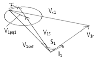
Figure 2. Phasor diagram of interline power flow controller
Let the proposed IPFC is made up of a series-connected VSC that may inject a voltage with adjustable amplitude and phase angle at the fundamental frequency while keeping the DC link voltage at a predetermined level [5-9]. For real power exchange across voltage sources, the common dc link is represented by a bidirectional link (P12 =P1pq = P2pq). A transmitting end bus with voltage Phasor V1s and a receiving end bus with voltage Phasor V1r make up the transmission line represented by reactance X1. Line2's transmitting end voltage Phasor is V2s, and the receiving end voltage Phasor is V2r, as represented by reactance X2. Simply put, both sending- and receiving-end voltages are assumed to be constant with fixed amplitudes, V1s = V1r = V2s = V2r =1pu., and fixed angles, resulting in equal transmission angles s1 = s2 for the two systems. The two line impedances are also expected to be equal, as is the rating of the two compensating voltage sources. This indicates that X1 equals X2 and V1pqmax equals V2pqmax. To derive the restrictions that the free controllability of system1 imposes on the power flow control of system2, it is assumed that system1 is chosen at random to be the principal system for which free controllability of both real and reactive line power flow is mandated. The connection between V1s, V1r, Vx1 and the inserted voltage phasor V1pq, with adjustable magnitude and angle, is defined by a phasor diagram of system1. The transmitting end voltage V1seff = V1s + V1pq is increased by V1pq. So the difference V1self –V1r establishes the corrected voltage phasor or Vx1 across reactance X1. End of phasor V1pq travels in a circle with its centre at end of phasor V1s as angle is changed across its full 360 degree range. The operational range of phasor V1pq is defined by the region within this circle. As a result, line 1 can be compensated. The magnitude and angle of phasor Vx1 are both modulated by the rotation with angle of phasor V1pq, and as a result, both the transmitted real power, P1r, and the reactive power, Q1r, fluctuate with 1 (Figure 2).
The IPFC is meant to keep the two transmission lines' impedance characteristics the same. The IPFC is made up of two converter systems: (a) a master converter system that can control both resistive and inductive impedances on Line 1; and (b) a slave converter system that controls Line 2 reactance and maintains the VSC's common dc-link voltage at a specified level. The slave units are energy gateway and microgrid. Slave converter system is supervised by a master controller which is local at PCC. Master can talk to slave via communication channel. As a result, each VSC may be controlled separately. In multi-level converters, balancing the dc voltages Vdc1 and Vdc2 on the capacitors C1 and C2, respectively, is critical. Over-voltages on the switching devices can be caused by uneven voltage charging on the capacitors, which can be dangerous. The equation for current through the transmission line with series compensation can be given as:
$I=\frac{V_X}{j X}=\frac{V_S^{\prime}-V_r}{j X}=\frac{V_S \angle 0+V_{S^{\prime} S} \angle \beta-V_r \angle-\delta}{j X}=\frac{V_S+V_{S^{\prime} S} \cos \beta+j V_{S^{\prime} S} \sin \beta-V_r \cos \delta+j V_r \sin \delta}{j X}=I \angle \theta_1$
where, $I=I \cos \theta_1+\mathrm{j} I \sin \theta_1$.
$I \cos \Theta_1=\frac{V_r \sin \delta+V_{S^{\prime} S} \sin \beta}{X}$ (1)
$I \sin \theta_1=\frac{V_r \cos \delta-V_S-V_{S^{\prime} S} \cos \beta}{X}$ (2)
The active power flow at the sending end with compensation can be given as: $P_s=V_S I \cos \left(\delta_S-\theta_I\right)$.
Combining the above two equations gives:
$P_s=\frac{V_S V_r}{X} \sin \delta+\frac{V_S V_{S^{\prime} S}}{X} \sin \beta$ (3)
$P_s=P_{s n}+A_s \sin \beta$ (4)
where, $A_s=\frac{V_S V_{S \prime S}}{X}$.
The reactive power flow at the sending end with compensation can be given as: $Q_S=V_S I \sin \left(\delta_S-\Theta_I\right)=-V_S I \sin \theta_I$.
Combining the above two equations gives:
$Q_s=\frac{-V_S V_r}{X} \cos \delta-\frac{V_S V_{S^{\prime}S}}{X} \cos \beta-V_S^2$ (5)
$Q_s=Q_{s n}+A_s \cos \beta$ (6)
where, $A_S=\frac{V_S V_{S^{\prime} S}}{X}$.
Rearranging the above equations gives:
$\left(P_S-P_{S n}\right)^2+\left(Q_S-Q_{S n}\right)^2=A_S^2$ (7)
$\frac{P_S-P_{S n}}{Q_S-Q_{S n}}=\tan \beta$ (8)
The above equation defines the relationship between $P_S$ and $Q_S$ as a circle centered at ($P_{S n}, Q_{S n}$) with a radius of $A_S$.
The magnitude of the compensating voltage can be given as:
$V_{S^{\prime} S}=\frac{X}{V_S} \sqrt{\left(P_S-P_{S n}\right)^2+}\left(Q_S-Q_{S n}\right)^2$ (9)
The relative phase angle can be given as:
$\beta=\tan ^{-1} \frac{P_S-P_{S n}}{Q_S-Q_{S n}}$ (10)
For $\beta=0$, the variations are $P_s$ and $Q_s$,
$\begin{aligned}& P_s=P_{s n}+A_s \sin 0=P_{s n}, \\& Q_s=Q_{s n}+A_s \cos 0=Q_{s n}+A_s\end{aligned}.$
For $\beta=180$, the variations are $P_s$ and $Q_s$,
$\begin{aligned}& P_s=P_{s n}+A_s \sin 180=P_{s n}, \\& Q_s=Q_{s n}+A_s \cos 180=Q_{s n}-A_s\end{aligned}.$
Power at receiving end: The active power flow at the receiving end with compensation can be given as:
$P_r=V_r I \cos \left(\delta_r-\Theta_I\right)$
$P_r=\frac{V_r V_r}{X} \cos \delta \sin \delta+\frac{V_r \cos \delta V_{S^{\prime} s}}{X} \sin \beta-V_r \sin \delta\left(\frac{V_r \cos \delta-V_s-\cos \beta V_{S^{\prime} S}}{X}\right) P_r=P_{r n}+A_r \sin (\delta+\beta)$ (11)
where, $A_r=\frac{V_r V_{S^{\prime} S}}{X}$.
The reactive power flow at the sending end with compensation can be given as:
$Q_r=V_r I \sin \left(\delta_r-\theta_I\right)=-V_r I \sin \left(\theta_I+\delta_r\right)$ (12)
Combining the above two equations gives:
$Q_r=-\frac{V_r V_r}{X} \sin \delta \sin \delta-\frac{V_r \sin \delta V_{S^{\prime} S}}{X} \sin \beta-V_r \cos \delta\left(\frac{V_r \cos \delta-V_s-\cos \beta V_{S^{\prime} S}}{X}\right) Q_s=Q_{r n}+A_r \cos (\beta+\delta)$ (13)
where, $A_r=\frac{V_r V_{S^{\prime} S}}{X}$.
Rearranging the above equations gives:
$\left(P_r-P_{r n}\right)^2+\left(Q_r-Q_{r n}\right)^2=A_r^2\frac{P_r-P_{r n}}{Q_r-Q_{r n}}=\tan (\delta+\beta)$ (14)
The above equation defines the relationship between $P_S$ and $Q_S$ as a circle centered at $\left(P_{S n}, Q_{S n}\right)$ with a radius of $A_s$.
The magnitude of the compensating voltage can be given as:
$V_{S \prime S}=\frac{X}{V_r} \sqrt{\left(P_r-P_{r n}\right)^2+}\left(Q_r-Q_{r n}\right)^2$ (15)
The relative phase angle can be given as:
$\beta=\tan ^{-1} \frac{P_r-P_{r n}}{Q_r-Q_{r n}}-\delta$ (16)
For $\beta=0$, the variations are $P_r$ and $Q_r$,
$\begin{aligned}& P_r=P_{r n}+A_r \sin (\delta+0)=P_{s n}+A_r \sin \delta, \\& Q_s=Q_{s n}+A_s \cos (\delta+0)=Q_{s n}+A_s \cos \delta .\end{aligned}$.
Feedback occurs when a system's outputs are redirected back as inputs as part of a cause-and-effect chain that creates a circuit or loop. In this instance, the gadget is said to feedback on itself. The feedback weighted link is a network in which the connections between nodes create a directed graph in time. This allows it to behave in a time-dependent manner. These are feed forward networks that use their internal state to process variable length sequences of inputs (memory). The phrase "feedback weighted relation" refers to two broad categories of networks that have a common overall structure, one with limited impulse and the other with infinite impulse. Both types of networks have a temporal hierarchical activity. A finite impulse feedback system is a directed acyclic diagram that can be unrolled and replaced with a strictly feed forward system, but an infinite impulse feedback network is a guided cyclic graph that cannot be unrolled and restored with a purely feed forward system. Each point's output is calculated using a non-linear function of its inputs, and the "signal" at each relation is a real integer. The connections are referred to as edges. The weight of inputs and edges varies as learning advances in most instances [10-15]. Depending on the weight, the signal intensity at a connection is raised or lowered. Systems are trained by examining examples with known "inputs" and "effects," establishing probability-weighted relationships between the two, and storing them in the network's information structure.
To train a device, the difference between the network's processed yield and a goal yield is typically utilized. Using this error number and a learning rule, the machine then updates its weighted correlations. The system can create output that becomes closer and closer to the intended output with each modification. After a fair number of these modifications have been made, the instruction will be cancelled depending on these circumstances. For a number of reasons, models may not always converge to a single solution. Local minima, for example, might arise depending on the cost function and the model. Second, the optimization procedure cannot ensure convergence when beginning far from any local minimum. Third, when dealing with large volumes of data or criteria, certain techniques become inefficient. The weighted feedback method has been broken down into the following phases. For the estimate of xi, y j, and zk, randomize weight (Wn), where n is the quantity of NBCC in the sample with a lot of space. It's time to figure out what Ra's best goal is. It is necessary to enter predictive models. If the projected output for the cutting combination xi, y j, and zkRa, then W new =(RaWold)/xiyjzk If this isn't the case, Wnew=Wold. Continue the process to complete the training.
With four algorithms: weighted feedback algorithm, gravitational search method, ant colony optimization algorithm, and BAT algorithm, the proposed power system was simulated with IPFC and evaluated with diverse test scenarios such as load switching, fault incidence, and control.
4.1 With fault condition in the power system
The LLL defect was introduced into the system at t=0.1s to t=0.65s, and several algorithms with IPFC were evaluated.
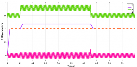
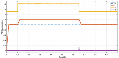
The weighted feedback algorithm was used to build the IPFC, and the Figure 3 below shows PCC characteristics including voltage, current, active strength, reactive power, and power factor under faulty situations using the IPFC.
Figure 3. PCC parameters of power system under faulted condition with WBA
The voltage has stayed nearly constant, also the current has stayed nearly the rated value, active power has grown to 0.1 times the rated value, and reactive power has been maintained to nearly zero.
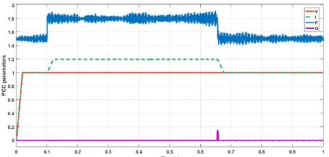
The GSA algorithm was used to implement the IPFC, and the Figure 4 below shows PCC characteristics such as voltage, current, active strength, reactive power, and power factor with IPFC under faulty circumstances.
Figure 4. PCC parameters of power system under faulted condition with GSA
The voltage has stayed nearly constant, where the current has increased to 20% of the rated value, active power has grown to 10% the rated value, and reactive power has been maintained to nearly zero.
The BAT method was used to implement the IPFC, and the Figure 5 shows PCC characteristics such as voltage, current, active strength, reactive power, and power factor with IPFC under faulty circumstances.
The voltage has stayed nearly constant, where the current has increased to 25% of the rated value, active power has grown to 20% the rated value, and reactive power has increased to 1%.
Figure 5. PCC parameters of power system under faulted condition with BAT
Figure 6. PCC parameters of power system under faulted condition with ANT
Table 1. PCC parameters with fault, DVR, GSA, BAT, ANT algorithms
|
Parameter |
Without facts devices |
Weighted feedback |
GSA |
BAT |
|
Voltage |
0.256pu |
1.00pu |
1.00pu |
0.99pu |
|
Current |
25.9pu |
1.01pu |
1.15pu |
1.18pu |
|
Active power |
10pu |
1.5pu |
1.73pu |
1.9pu |
|
Reactive power |
0pu |
0pu |
0pu |
0.1pu |
|
Power factor |
0.99pu |
1.00pu |
0.99pu |
0.99pu |
The ANT COLONY algorithm was used to implement the IPFC, and the Figure 6 below shows PCC characteristics such as voltage, current, active strength, reactive power, and power factor with IPFC under faulty circumstances.
The voltage has stayed nearly constant, where the current has increased to 25% of the rated value, active power has grown to 22% the rated value, and reactive power has been maintained to nearly zero with overshoot at sudden closure of loads. Table 1 shows the PCC parameters under fault condition with the four algorithms.
The above table shows the perfromance of various algortihms based IPFC under faulted condition in terms of various parameters like voltage, current, active power, reactive power and power factor at the point of common coupling.
4.2 With wind-based induction generator
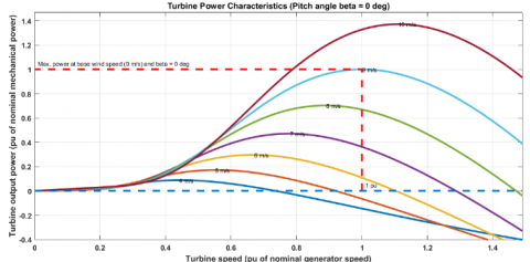
A wind turbine-based induction generator was connected to the grid at t=0.1s to t=0.65s, and several algorithms with IPFC were evaluated as in Figure 7.
Under abrupt turbine switching situations, the Figure 8 below displays PCC characteristics such as voltage, current, active power, reactive capacity, and power factor using IPFC utilizing the weighted feedback method.
The voltage has stayed nearly constant, the current has increased to 5% of the rated value, active power has grown to 10% the rated value, and reactive power has been maintained to nearly zero with smaller overshoot at sudden closure of loads.
Under abrupt turbine switching situations, the Figure 9 below displays PCC characteristics such as voltage, current, active power, reactive capacity, and power factor using IPFC utilizing the GSA algorithm.
The voltage has stayed nearly constant, where the current has increased to 20% of the rated value, active power has grown to 27% the rated value, and reactive power has been maintained to nearly zero with overshoot at sudden closure of loads.
Under abrupt turbine switching situations, the Figure 10 below displays PCC characteristics such as voltage, current, active power, reactive capacity, and power factor using IPFC utilizing the BAT algorithm.
The voltage has stayed nearly constant, where the current has increased to 30% of the rated value, active power has grown to 30% the rated value, and reactive power has been maintained to nearly zero with overshoot at sudden closure of loads.
Under abrupt turbine switching situations, the Figure 11 displays PCC characteristics such as voltage, current, active power, reactive capacity, and power factor using IPFC utilizing the ANT COLONY algorithm.
The voltage has stayed nearly constant, where the current has increased to 40% of the rated value, active power has grown to 35% the rated value, and reactive power has been maintained to nearly zero with overshoot at sudden closure of loads. Table 2 shows the PCC parameters under induction with the four algorithms.
Figure 7. Speed vs output for wind turbine
Figure 8. PCC parameters of power system under sudden switching condition WBA
Figure 9. PCC parameters of power system under sudden switching condition with GSA
Figure 10. PCC parameters of power system under sudden switching condition with BAT
Table 2. PCC parameters with induction generator, DVR, GSA, BAT, ANT algorithms
|
Parameter |
Without Facts |
Weighted Feedback |
GSA |
BAT |
ANT |
|
Voltage |
0.935pu |
1.00pu |
1.00pu |
1.00pu |
1.00pu |
|
Current |
2pu |
1.02pu |
1.2pu |
1.27pu |
1.326pu |
|
Active Power |
2.4pu |
1.54pu |
1.8pu |
1.92pu |
2.0pu |
|
Reactive Power |
1.5pu |
0.001pu |
0.001pu |
0.002pu |
0.005pu |
|
Power Factor |
0.5pu |
1.0pu |
0.996pu |
0.994pu |
0.99pu |
Figure 11. PCC parameters of power system under sudden switching condition with ANT
The above table shows the perfromance of various algortihms based IPFC under sudden swicthing of induction loads condition in terms of various parameters like voltage, current, active power, reactive power and power factor at the point of common coupling.
4.3 With wind based synchronous generator
The wind turbine-based synchronous generator was connected to the grid at t=0.1s to t=0.65s, and several algorithms with IPFC were evaluated.
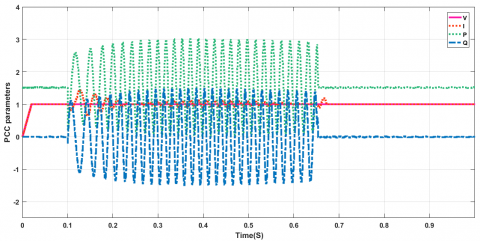
The IPFC was implemented using the weighted feedback method, and the Figure 12 depicts the PCC characteristics such as voltage, current, active intensity, reactive capacity, and power factor under IPFC-enabled abrupt turbine switching situations.
The voltage has stayed nearly constant, where the current has increased to 10% of the rated value, active power has grown to 90% the rated value with oscillations, and reactive power has grown to 90% the rated value with oscillations.
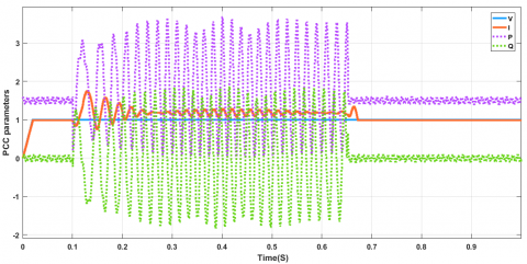
Figure 13 displays the PCC characteristics such as voltage, current, active intensity, reactive capacity, and power factor under abrupt turbine switching situations using IPFC using the GSA algorithm.
The voltage has stayed nearly constant, where the current has increased to 15% of the rated value, active power has grown to 95% the rated value with oscillations, and reactive power has grown to 95% the rated value with oscillations.
The BAT method was utilized to implement the IPFC, and the Figure 14 below depicts PCC characteristics such as voltage, current, active intensity, reactive capacity, and power factor during IPFC-assisted abrupt turbine switching.
The IPFC was implemented using the ANT COLONY algorithm, and the Figure 15 depicts PCC characteristics such as voltage, current, active intensity, reactive capacity, and power factor under IPFC under abrupt turbine switching situations.
Figure 12. PCC parameters of power system under sudden switching condition of synchronous loads with WBA
Figure 13. PCC parameters of power system under sudden switching condition of synchronous loads with GSA
Figure 14. PCC parameters of power system under sudden switching condition of synchronous loads with BAT
Figure 15. PCC parameters of power system under sudden switching condition of synchronous loads with ANT
Table 3. PCC parameters with synchronous generator, DVR, GSA, BAT, ANT algorithms
|
Parameter |
Without Facts |
Weighted Feedback |
GSA |
BAT |
ANT |
|
Voltage |
0.98pu |
1.0pu |
1.05pu |
1.06pu |
1.09pu |
|
Current |
1.249pu |
1.2pu |
1.3pu |
1.2pu |
1.3pu |
|
Active Power |
1.81pu |
3.0pu |
3.35pu |
3.8pu |
3.7pu |
|
Reactive Power |
0.4pu |
1.5pu |
1.6pu |
1.65pu |
1.7pu |
|
Power Factor |
0.98pu |
0.99pu |
0.98pu |
0.975pu |
0.971pu |
The voltage has stayed nearly constant, where the current has increased to 10% of the rated value, active power has grown with oscillations, and reactive power has grown with oscillations. Table 3 shows the PCC parameters under synchronous generator with the four algorithms.
The above table shows the performance of various algorithms based IPFC under sudden switching of synchronous loads condition in terms of various parameters like voltage, current, active power, reactive power and power factor at the point of common coupling.
4.4 With RLC load
At t=0.1s to t=0.65s, the RLC load was attached to the system, and several methods with IPFC were tried.
The IPFC was designed using the Weighted Feedback Algorithm, and the Figure 16 below shows the PCC parameters with the RLC load linked to the IPFC.
The voltage, current, active power and reactive power are nearly maintained constant.
Figure 16. PCC parameters of power system under sudden switching condition of RLC loads with WBA
The GSA Algorithm was used to calculate the IPFC parameters, and the Figure 17 below shows the PCC parameters with the RLC load linked to the IPFC.
The voltage has stayed nearly constant, where the current has increased to 5% of the rated value, active power has grown to 10% the rated value, and reactive power has been maintained to nearly zero with overshoot at sudden closure of loads.
The BAT Algorithm was used to calculate the IPFC parameters, and the Figure 18 below shows the PCC parameters with the RLC load linked to the IPFC.
The voltage has stayed nearly constant, where the current has increased to 10% of the rated value, active power has grown to 15% the rated value, and reactive power has been maintained to nearly zero with overshoot at sudden closure of loads.
The ANT COLONY Algorithm was utilized for the IPFC, and the Figure 19 below shows the PCC parameters with the IPFC's RLC load attached.
Figure 17. PCC parameters of power system under sudden switching condition of RLC loads with GSA
Figure 18. PCC parameters of power system under sudden switching condition of RLC loads with BAT
Table 4. PCC parameters with RLC load, DVR, GSA, BAT, ANT algorithms
|
Parameter |
Without Facts |
Weighted Feedback |
GSA |
BAT |
ANT |
|
Voltage |
0.998pu |
1pu |
1.00pu |
1.00pu |
0.995pu |
|
Current |
1.018pu |
1pu |
1.05pu |
1.064pu |
1.076pu |
|
Active Power |
1.526pu |
1.53pu |
1.57pu |
1.61pu |
1.7pu |
|
Reactive Power |
0.0001pu |
0pu |
0pu |
0.001pu |
0.001pu |
|
Power Factor |
0.999pu |
1.00pu |
1.00pu |
0.999pu |
0.99pu |
Figure 19. PCC parameters of power system under sudden switching condition of RLC loads with ANT
The voltage has stayed nearly constant, where the current has increased to 10% of the rated value, active power has grown to 15% the rated value, and reactive power has been maintained to nearly zero with overshoot at sudden closure of loads. Table 4 shows the PCC parameters under RLC load with the four algorithms. The Table 4 shows the performance of various algorithms based IPFC under sudden switching of RLC loads condition in terms of various parameters like voltage, current, active power, reactive power and power factor at the point of common coupling.
The notion of an interline power flow controller based on the VSC theorem is investigated and built in this article. In this article, four distinct algorithms are used to control the PCC parameters as well as the IPFC output. A comparison of all four IPFC algorithms in terms of voltage, current, active power, reactive power, and power factor was also conducted, with the weighted feedback algorithm beating the others under various test circumstances. The entire system was built and examined using MATLAB simulation and code. The outcome of the simulation shows that the proposed algorithm succeeds in terms of in terms of current, voltage, active power, reactive power, and power factor. In future we plan to investigate the performance of the proposed work with various machine learning techniques.
[1] Yi, J., Zhu, M., Zhong, X., et al. (2020). An improved triple interline DC power flow controller for bidirectional power control. In 2020 IEEE Region 10 Conference (Tencon), Osaka, Japan, pp. 1301-1306. https://doi.org/10.1109/TENCON50793.2020.9293704
[2] Chen, W., Zhu, X., Yao, L., et al. (2016). A novel interline DC power-flow controller (IDCPFC) for meshed HVDC grids. IEEE Transactions on Power Delivery, 31(4): 1719-1727. https://doi.org/10.1109/TPWRD.2016.2547960
[3] Zhong, X., Zhu, M., Huang, R., Cai, X. (2017). Combination strategy of DC power flow controller for multi-terminal HVDC system. The Journal of Engineering, 2017(13): 1441-1446. https://doi.org/10.1049/joe.2017.0570
[4] Sau-Bassols, J., Prieto-Araujo, E., Gomis-Bellmunt, O. (2017). Modelling and control of an interline current flow controller for meshed HVDC grids. IEEE Transactions on Power Delivery, 32(1): 11-22. https://doi.org/10.1109/TPWRD.2015.2513160
[5] Egea-Alvarez, A., Bianchi, F., Junyent-Ferré, A., Gross, G., Gomis-Bellmunt, O. (2012). Voltage control of multiterminal VSC-HVDC transmission systems for offshore wind power plants: Design and implementation in a scaled platform. IEEE Transactions on Industrial Electronics, 60(6): 2381-2391. https://doi.org/10.1109/TIE.2012.2230597
[6] Mu, Q., Liang, J., Li, Y., Zhou, X. (2012). Power flow control devices in DC grids. In 2012 IEEE Power and Energy Society General Meeting, San Diego, CA, USA, pp. 1-7. https://doi.org/10.1109/PESGM.2012.6345674
[7] Khatoon, N., Shaik, S. (2017). A survey on different types of flexible AC transmission systems (facts) controllers. International Journal of Engineering Development and Research, 5(4): 796-814.
[8] Bharti, H., Arya, J.S., Arya, A.K. (2018). Power loss minimization with multiple DG in distribution system using gravitational search algorithm. IJEDR, 6(3): 101-106.
[9] Kumar, L., Kumar, S., Gupta, S.K., Raw, B.K. (2019). Optimal location of FACTS devices for loadability enhancement using gravitational search algorithm. In 2019 IEEE 5th International Conference for Convergence in Technology (I2CT), Bombay, India, pp. 1-5. https://doi.org/10.1109/I2CT45611.2019.9033561
[10] Zhang, J., Liu, K., Liu, Y., He, S., Tian, W. (2019). Active power decoupling and controlling for single-phase FACTS device. The Journal of Engineering, 2019(16): 1333-1337. https://doi.org/10.1049/joe.2018.8823
[11] Loubna, K., Bachir, B., Izeddine, Z. (2018). Optimal digital IIR filter design using ant colony optimization. In 2018 4th International Conference on Optimization and Applications (ICOA), Mohammedia, Morocco, pp. 1-5. https://doi.org/10.1109/ICOA.2018.8370500
[12] Kritele, L., Benhala, B., Zorkani, I. (2017). Ant colony optimization for optimal analog filter sizing. Focus on Swarm Intelligence Research and Applications, pp. 193-220.
[13] Chandra Sekhar, D., Rama Rao, P.V.V, Ganesh, V. (2019). Weight feedback adaptive multi objective cooperative scheduling in smart grid application. International Journal of Recent Technology and Engineering (IJRTE), 8(2): 607-611. https://doi.org/10.35940/ijrte.b1634.078219
[14] Behuria, A., Mishra, B. P., Goel, P., Kar, A., Mohapatra, S., Chandra, M. (2015). A novel variable step-size feedback Filtered-X LMS algorithm for acoustic noise removal. In 2015 International Conference on Advances in Computing, Communications and Informatics (ICACCI), Kochi, India, pp. 166-171. https://doi.org/10.1109/ICACCI.2015.7275603
[15] Kar, A., Chanda, A.P., Mohapatra, S., Chandra, M. (2014). An improved filtered-x least mean square algorithm for acoustic noise suppression. Advanced Computing, Networking and Informatics, 1: 25-32. https://doi.org/10.1007/978-3-319-07353-8_4