Isa Ataş
© 2022 IIETA. This article is published by IIETA and is licensed under the CC BY 4.0 license (http://creativecommons.org/licenses/by/4.0/).
OPEN ACCESS
Panoramic Dental Radiography (PDR) image processing is one of the most extensively used manual methods for gender determination in forensic medicine. With the assistance of the PDR images, a person's biological gender determination can be performed through analyzing skeletal structures expressing sexual dimorphism. Manual approaches require a wide range of mandibular parameter measurements in metric units. Besides being time-consuming, these methods also necessitate the employment of experienced professionals. In this context, deep learning models are widely utilized in the auto-analysis of radiological images nowadays, owing to their high processing speed, accuracy, and stability. In our study, a data set consisting of 24,000 dental panoramic images was prepared for binary classification, and the transfer learning method was used to accelerate the training and increase the performance of our proposed DenseNet121 deep learning model. With the transfer learning method, instead of starting the learning process from scratch, the existing patterns learned beforehand were used. Extensive comparisons were made using deep transfer learning (DTL) models VGG16, ResNet50, and EfficientNetB6 to assess the classification performance of the proposed model in PDR images. According to the findings of the comparative analysis, the proposed model outperformed the other approaches by achieving a success rate of 97.25% in gender classification.
DenseNet121, deep convolutional neural network, deep transfer learning, gender prediction, panoramic dental radiograph
Nowadays, artificial intelligence is actively used in a variety of domains, particularly in health [1, 2], industry [3], natural language processing [4], generative networks [5], remote sensing [6] etc. However, the modern methods developing rapidly in artificial intelligence technologies have shown remarkable success in image analysis and become more effective in medical applications. This study is based on the ground of the convolutional neural network, which has provided successful results in various image analyses with modern methods. Our dataset consists of 24,000 PDR images acquired from the local patients.
In the events where a significant number of mortalities occur as a consequence of natural disasters or catastrophes, making identification on human residue is necessary through the participation of professionals from various occupational groups. Due to the exposure of human remains to extreme and destructive external forces and their biological decomposition, making such identifications based on the existing remains becomes a challenging process [7]. The 2014 INTERPOL Disaster Victim Identification Standards emphasizes that DNA analysis, friction ridge analysis, and forensic dental study methods are the primary, most reliable, and efficacious description techniques [8]. The determination of biological gender is the initial stage in the identification process.
Gender identification from human skeletal remains has been identified as an important factor in forensic science and bio-archaeology [9]. When determining gender in the defined areas, it is necessary to use as many methods or features as possible instead of using a single morphological feature as a reference [10]. In the literature, studies have been carried out for sex prediction with all existing bones of the human skeleton. mandible [11], calcaneus [12], metatarsal bone and phalanx [13], femur [9], patella [14], occipital condyle [15], hand bones [16] and sternum [17] are used to predict gender [18].
Despite the adversities, the mandible, which is usually known as the strongest, largest, and most resistant bone that remains intact, plays a significant role in gender prediction in forensic odontology [19, 20]. Therefore, the mandible, a skeletal component, is the focus.
Rather than taking a single morphological character as a reference, it is necessary to use as many procedures or features as possible while determining the gender of the unknown skeletal residues [10]. The PDR images with the mandible may provide information about dental status, age range, and gender. It is also conceivable to perform identification of a dead body or living individual whose identity is unknown, with such limited data on hand. Many diverse manual techniques are employed for gender prediction from PDR images of teeth. For instance, while an adult’s skull is a reference material to identify gender with an accuracy of 80%, this accuracy can rise to 90% when the mandible is taken into account, additionally [21, 22]. Although manual approaches are prone to error, the application of the aforementioned techniques requires a certain amount of time and experienced specialists (forensic anthropologist, pathologist, etc.) who are familiar with such techniques [23, 24].
As a result, the PDR images, acquired with fully automatic image techniques, covering the entire mandible and contributing positively to biometric identification; and thereby providing a holistic approach, were used for gender classification in our study.
It is possible to identify gender and age from skeletal remains in forensic medicine, osteology, and physical anthropology; however, gender determination by age is considered the most challenging issue [25]. The mandible reflects the anatomical distinctions between male and female individuals and poses sexual differentiation based on morphological characters [26]. The process of manually separating morphological characters for gender classification is common. Due to the intricacy of PDR images, researchers mostly concentrate on different morphometric and non-metric parameters of the mandible [27-29]. As a result of morphometric studies, Loth et al. achieved over 90% classification success as grounding on the characteristic of the ramus flexure, which is absent in males but is present in female individuals and is also regarded as a part of the mandible [30-33]. Lin et al. set the upper limit of mandibular flexure, the maximum ramus vertical height, and upper ramus vertical height as discrimination parameters and correctly classified 81.7% to 88.8% gender classification among 240 three-dimensional mandibular models [11]. Deana and Alves utilized numerous characteristics in non-metric studies, including jaw shape, eversion of the gonial angle, jaw profile, contour of the base of the mandible, and shape of the ramus, and reported a gender classification rate with an accuracy ranging from 75% to 95.2% [34]. Nagaraj et al. studied mandibular ramus flexure on a digital orthopantomogram. Statistical analysis was performed using SPSS software on the data of 100 subjects, and 71% accuracy was obtained [35]. In the cited manual studies in the literature, there were intact mandibles used without any pathology, loss of mandibular molars or abnormal molars, and teeth. Milošević et al. proposed an automated solution for gender estimation based on deep learning techniques using convolutional neural networks from PDR images instead of employing only specific metric and non-metric indicators. However, as the test dataset advanced from 400 to 2000, the accuracy rate reduced from 96.8% to 92.3% [7]. Ivan et al. used deep convolutional neural networks (DCNN), which have attested successfully in image analysis, and achieved 94.3% accuracy in the test dataset used in DCNN models [21]. Based on the convolutional neural network developed by a multi-feature fusion module, Ke et al. suggested a new automated technique for gender estimation from panoramic dental x-ray images. With the method proposed, they attained 94.6% ±0.58% accuracy on the test dataset they used [36]. Ortiz et al. propounded a new technique for gender estimation through anatomical points that appear on panoramic radiographs using machine learning techniques. The accuracy rate was 68% for women and 74% for men [37]. The novel methods reported in the literature for gender estimation are mainly based on deep learning approaches and do not require any manual feature adjustment.
In addition to these studies, preprocessing techniques to improve the quality of dental images by years are presented in Table 1, various studies in dentistry that consider deep learning-based techniques are presented in Table 2 and the development criteria of dental X-ray imaging techniques are presented in Table 3 [38].
Table 1. Preprocessing techniques on dental images
|
Author - Year |
Related studies |
Application |
|
Patanachai et al. [39] - 2010 |
Standard and adaptive with wavelet transform thresholding segmentations are compared and applied. |
Teeth detection |
|
Frejlichowski and Wanat [40] - 2011 |
In the automatic approach, a horizontal integral projection is applied to segment the teeth. |
Human identification |
|
Pushparaj et al. [41] - 2013 |
Horizontal integral projection with a B-spline curve is employed to separate maxilla and mandible. |
Teeth numbering |
|
Lira et al. [42] – 2014 |
Supervised learning used for segmentation and feature extraction is carried out through computing moments and statistical characteristics. |
Teeth detection |
|
Abdi et al. [43] – 2015 |
Segmentation processes for gap valley extraction, contour tracing and template matching are applied. |
Mandible detection |
|
Poonsri et al. [44] - 2016 |
Area segmentation using K-means clustering and template matching using correlation are applied. |
Teeth detection |
|
Zak et al. [45] - 2017 |
Adaptive individual arch tooth segmentation thresholding is applied to locate the palatal bone. |
Teeth detection |
|
Mahdi and Kobashi [46] - 2018 |
Quantum particle swarm optimization is applied for multi-level thresholding. |
Teeth detection |
|
Fariza et al. [47] - 2019 |
Gaussian kernel-based conditional in segmentation operation spatial fuzzy c-means algorithm is applied. |
Teeth detection |
|
Aliaga et al. [48] - 2020 |
Segmentation from X-ray images is performed using k-means clustering. |
Mandible detection |
|
Esmaeilyfard et al. [49] - 2021 |
Naive Bayesian (NB), Random Forest (RF) and Support Vector Machine (SVM) are used as classifiers for prediction. |
Teeth detection |
Table 2. Different teeth studies based on machine learning
|
Author - Year |
Models |
Application |
Evaluation |
|
Oktay [50] - 2017 |
AlexNet |
Detection and classification |
Accuracy |
|
Chu et al. [51] - 2018 |
Octuplet siamese network |
Osteoporosis analysis |
Accuracy |
|
Lee et al. [52] - 2019 |
Mask R-CNN |
Segmentation for diagnosis and forensic identification |
F1 score |
|
Muramatsu et al. [53] - 2020 |
CNN (ResNet50) |
Detection and classification |
Confusion Matrix |
|
Esmaeilyfard et al. [49] - 2021 |
Support Vector Machine (SVM) |
Detection and classification |
Accuracy |
Table 3. Developmental stages of Dental X-ray imaging techniques
|
Year |
Dental imaging methods |
|
2005 |
Level Set method |
|
2006 |
Mathematical morphology & Connect component labelling |
|
2007 |
Four field transformation & Support vector machine |
|
2008 |
Clustering & Region growing |
|
2009 |
Automatic iterative point correspondence algorithm & Hybrid knowledge acquisition |
|
2010 |
Histogram based & Wavelet transform |
|
2011 |
Canny, Sobel, Gaussian, Laplacian, Avarage filtering & Active contour |
|
2012 |
Homomorphic filter, Distance, Adaptive windowing & Phase Congruency |
|
2013 |
Harris operator, SVM Classifier & Gray-level co – occurrence matrix |
|
2014 |
Bayesian Classifier, Gaussian filter & Local singularity analysis |
|
2015 |
Cluster based Segmentation & Active shape model |
|
2016 |
Fuzzy C-means & U-net architecture |
|
2017 |
Neutrosophic Orthogonal Matrices, Transfer learning & Machine learning |
|
2018 |
Multi-layer perceptron, Backpropagation algorithm & Deep learning-based CNN |
|
2019 |
Multilayer perceptron, Auto Regression model & Geodesic active contour |
|
2020 |
Deep Convolution Neural Network |
|
2021 |
Deep Convolution Neural Network & Transformer |
3.1 Dataset collection and preparation
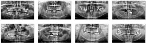
For binary classification of the PDRs, a dataset of images and label pairs was constructed and structurally tested by training in four alternative deep learning network architectures (VGG [54] – ResNet [55] – EfficientNet [56] – DenseNet [57]). This study examined a dataset of 24,000 PDR images from patients aged between 18 and 77 who received dental treatment in Diyarbakir Oral and Dental Health Hospital Periodontology clinic between 2015 and 2020. The female and male patient ratio in the data set was 58% and 42%, respectively. The images were captured using the Promax 2D digital panoramic x-ray machine (anodic voltage 50-84 KV, current 0.5-16 mA, Planmeca, Finland) available in the clinic. The acquired PDR pictures had considerable differences in terms of contrast, location, and resolution parameters. That variation was one of the factors complicating gender identification. Figure 1 and Figure 2 illustrates sample female and male PDR images taken from a variety of patients. The PDR images were pre-processed to reduce complexity and focus on the mandible area. The histogram equalization method was applied to interpret the mandible area and teeth.
Furthermore, the resolution of original PDR images was resized from 3180 × 1509 to 224 × 224 pixels for the deep learning model without interfering with the aspect ratio value. An Open CEZERI Library (OCL) was utilized for pre-processing [58].
Table 4 lists the distribution of the PDR image dataset 64%, 16%, 20% as training, validation and test set, respectively.
It is clear from the histogram graph that the number of patients aged between 25 and 50 are higher than the others.
Figure 1. Sample PDR images of female patients by gender
Figure 2. Sample PDR images of male patients by gender
Table 4. Training, validation and testing rates by gender in the PDR image dataset
|
Class label |
Train (64%) |
Validation (16%) |
Test (20%) |
Total (100%) |
|
Female |
8,960 |
2,240 |
2,800 |
14,000 |
|
Male |
6,400 |
1,600 |
2,000 |
10,000 |
|
Total |
15,360 |
3,840 |
4,800 |
24,000 |
3.2 Transfer learning
Transfer learning is a deep learning method in which model parameters are used on a large pre-trained dataset. In other words, transfer learning is a machine learning technique in which we reuse a trained model defined as the starting place for a model in a new position. Transfer learning is used in problems where there is not enough data for training or we want better results in a short time. Figure 3 shows the transfer learning procedure.
Figure 3. Transfer learning procedure
3.3 Proposed model
Convolution in the training of the convolutional neural networks and increment in subsampling steps causes a decrease in feature maps. However, gradient loss occurs in the image feature during transitions between cross-layers. The DenseNet architecture, in particular, was created to take advantage of the feature maps more effectively [57]. Each dense block in the DenseNet architecture has two convolution layers (conv), which are comprised of a varying number of repetitions. These are the 1 × 1 dimensional core defined as the bottleneck layer and the 3 × 3 dimensional core that will perform the convolution process. A 1x1 convolution layer is introduced before each 3 × 3 convolution layer to improve computational efficiency; thus, the number of input feature maps is reduced. However, each transitional layer contains a 1 × 1 convolution layer and a 2 × 2 average pooling layer with two strides [57].
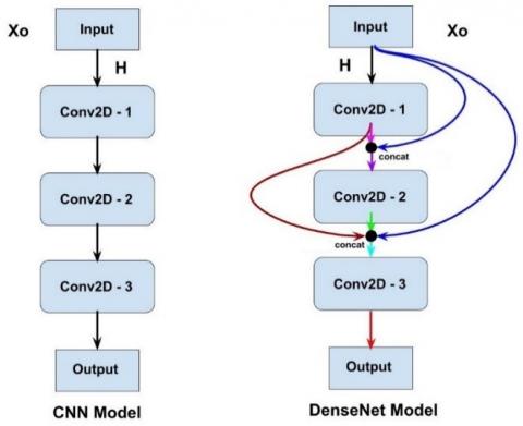
Figure 4. General CNN (left) and DenseNet (right) models
In the classical CNN architecture, while each layer only has information about the feature map received from the previous layer, in the DenseNet architecture, however, each layer is updated with the inputs of all back layers. Since each layer is coupled feed-forwardly to others, any layer can access the feature information of all preceding layers. Reutilization of the feature map in dense blocks by different layers boosts the input and performance of the next layer, allowing for the generation of easy-to-train models. Figure 4 shows the comparison of the classical CNN model with the DenseNet model. When analyzing layer three in Figure 4, the DenseNet model is comprehended to receive information from all back layers, whereas the CNN model only gets input from the preceding layer, which is layer two. Using such a strategy improves the flow of information and feature maps in the DenseNet, resulting in a minimum loss. Several variants have been designed that belongs to the DenseNet family including DenseNet121, DenseNet169, and DenseNet201 [57].
When the feature coupling is mathematized; if X0 is defined as the input image, then the H can be defined as a composite function consisting of three consecutive steps. In other words, H, the transfer function, consists of a combination of batch normalization (BN), rectified linear unit (ReLU), and 3 × 3 convolution (Conv.).
For the general CNN, while l’th output is generated by the l-1‘th input,
$X_l=H_l\left(X_{l-1}\right)$ (1)
In the DenseNet architecture, each layer concatenates the feature maps of previous layers and uses them as input for itself. Thus, l' th output is used as $X_0, \ldots, X_{l-1}$ input via taking the feature maps of all preceding layers and defining them as their assembly.
$X_l=H_l\left(\left[X_0, X_1, X_2, \ldots, X_{l-1}\right]\right)$ (2)
In the DenseNet, the size of the feature map expands as it passes through each dense layer and compiles existing features (the k parameter) from previous layers. The growing rate indicated by the parameter 'k' defines how dense architecture produces the most advanced outcomes. Thanks to the concatenate node built between the layers, the DenseNet performs well enough, despite having fewer parameters than the classical CNN architecture. The DenseNet121 model we proposed achieved better performance with approximately 7M parameters when compared to other models we tested in binary classification analysis. If every l’th layer of H generates k unit of the feature map, then l’th layer can be defined as:
$k_l=k_0+k \times(l-1)$ (3)
Here, k0 refers to the number of channels in the input layer [57].
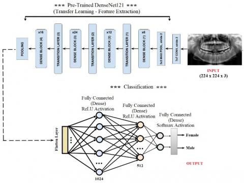
This study proposed a deep transfer learning strategy of the pre-trained DenseNet121 model to conduct binary classification from the PDR images. The proposed model was trained specifically with our PDR image set. The architecture of the DenseNet121 model is depicted in Figure 5.
The adjusted hyper-parameters of our model consisted of the learning rate, batch size, dropout rate, number of epochs, and optimizer. Table 2 lists the hyper-parameters used to train the proposed deep transfer model. In the performance analysis, the best accuracy rate with the minimum loss was attained using the values provided in Table 5. The Adam optimizer algorithm was used to optimize several DCNN models containing medical images [59].
In addition, when compared to other optimizers such as Stochastic Gradient Descent (SGD) [60] and RMSProp [61], the Adam optimizer had an appropriate function with minimal memory consumption and fast convergence. Our test dataset had approximately 4,800 PDRs, and such an amount could be regarded within the range of an adequate number to evaluate the performance of a gender estimation.
Table 5. Selected hyper-parameters to train the proposed deep transfer model
|
Hyper-parameters |
Options |
|
Learning rate |
0.0001 |
|
Batch size |
16 |
|
Dropout rate |
0.5 |
|
Epochs |
50 |
|
Optimizer |
Adam |
Figure 5. Architecture of proposed DenseNet121 deep transfer learning model for gender classification
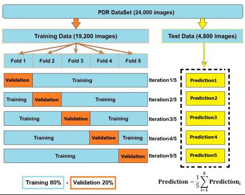
In our study, a 5-fold cross-validation technique was used to avoid overfitting or bias and to evaluate model training [62]. The 19,200 images allocated for the training dataset are divided into five layers, and the dataset of each layer was sliced into 80 to 20 percent slices. The model was established using the train set in all steps and evaluated with the validation set. The statistical summary of the evaluation scores of the model was examined. The 5-fold cross-validation technique is presented in Figure 6. These steps were repeated for the specified models (VGG16, ResNet50, EfficientNetB6 and DenseNet121) and the averages found as a result of the trials were reflected in the tables.
The analyzes made in the study were evaluated on the Google Colab cloud platform [63] with 13,342 RAM - Tesla K80 GPU - NVIDIA T4 GPUs Card.
3.4 Evaluation metrics
The confusion matrix is one of the most significant performance criteria in multi-classification problems. In this context, the accuracy, sensitivity, specificity, recall, and F1 score criteria are calculated through the confusion matrix [64]. The confusion matrix expresses the accuracy of the classifier by comparing the actual and predicted label values. Table 6 shows the general structure of a confusion matrix.
True positive (TP) and true negative (TN) are where the model predicts the correct answer; false positive (FP) and false negative (FN) are where the model gets it wrong.
TP: Female data was estimated accurately and assigned as a true-positive label.
FP: Female data was estimated as Male and assigned as a false-positive label.
FN: Male data was estimated as Female and assigned as a false-negative label.
TN: Male data was estimated accurately and assigned as a true-negative label.
The accuracy refers to the ratio of correct (true) data defined to all data used. It is calculated as follows [64].
Figure 6. The overview of the performed 5-fold cross validation in this study
Table 6. Confusion matrix
|
|
Predict Label |
||
|
Actual Label |
|
Female |
Male |
|
Female |
True Positive (TP) |
False Negative (FN) |
|
|
Male |
False Positive (FP) |
True Negative (TN) |
|
Accuracy $=\frac{(T P+T N)}{(T P+T N+F P+F N)}$ (4)
The precision refers to the ratio of positive data identified as true to all data identified as true. It is calculated as follows [64].
Precision $=\frac{T P}{(T P+F P)}$ (5)
The specificity refers to the ratio of negative data defined as true to the sum of negative data defined as true and positive data defined as false. It is calculated as follows [64].
Specifity $=\frac{T N}{(T N+F P)}$ (6)
The recall refers to the ratio of positive data identified as true to the sum of positive data identified as true and negative data identified as false. It is calculated as follows [65].
Recall $=\frac{T P}{(T P+F N)}$ (7)
The F1 Score metric is used when calculating the harmonic mean, which requires precision [64].
F1 Score $=2 \times \frac{ { Precision } \times { Recall }}{ { Precision }+ { Recall }}$ (8)
In this section, the VGG16, ResNet50, and EfficientNetB6 models, commonly used as transfer learning models, were compared with the DenseNet121 model, which was recommended for binary classification from PDR images.
Table 7 illustrates the test accuracy values for the DenseNet models (121-169-201). With the highest accuracy value among the compared ones, the DenseNet121 model came to the forefront. Furthermore, the DenseNet121 was utilized as a reference model for the binary classification of PDR pictures due to its modest number of parameters. The accuracies of the proposed models were compared at various image resolutions for gender prediction, and the result was given in Table 8. The accuracy was significantly lower at the resolution of 96 × 96. Therefore, the 224 × 224 PDR resolution was preferred for comparative analysis in the study.
Table 7. Comparison of DenseNet models for test accuracy values
|
Model |
Total Parameters |
Accuracy |
|
DenseNet121 |
8,617,026 |
0.9725 |
|
DenseNet169 |
14,880,322 |
0.9345 |
|
DenseNet201 |
20,822,594 |
0.9467 |
Table 8. Comparison of the proposed model's accuracy at different image resolutions
|
Model |
Resolution of PDR |
Accuracy |
|
DenseNet121 |
96 × 96 |
0.8734 |
|
DenseNet121 |
128 × 128 |
0.9233 |
|
DenseNet121 |
224 × 224 |
0.9725 |
Table 9 shows the performance accuracy values for the test dataset of the four models compared. The selected hyper-parameters were employed in the training of four deep transfer learning. It was noteworthy that the accuracy value of the VGG16 was dramatically low. The DenseNet121 model, however, had the highest accuracy value among all the models.
The DenseNet121 architecture was compared with a different number of network layers. The results in Table 10 show that increasing or decreasing the number of network layers symmetrically has little effect on the accuracy of gender inference.
Table 9. Comparison of deep transfer learning models
|
DTL model |
Input shape |
Total parameters |
Accuracy |
|
VGG16 |
(224, 224, 3) |
15,767,874 |
0.8220 |
|
ResNet50 |
(224, 224, 3) |
26,219,906 |
0.9260 |
|
EfficientNetB6 |
(224, 224, 3) |
43,855,505 |
0.9400 |
|
DenseNet121 |
(224, 224, 3) |
8,617,026 |
0.9725 |
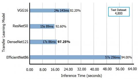
The test inference times of the compared models is depicted in Figure 7.
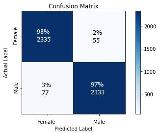
In the confusion matrix, the influence of false-positive and false-negative rates was presented in Figure 8. The Densenet121 model was found to generate minimal false-negative and false-positive results. For a visual representation of how successfully the DenseNet121 model identified samples for validation, the confusion matrix was employed. Table 11 shows the confusion matrix summary for the proposed model and previous deep learning-based PDR classification algorithms. The proposed model correctly classified 97.25% of the samples.
Figure 7. The elapsed inference times for the proposed transfer learning models
Figure 8. Confusion matrix analyses of the proposed model
When estimating the PDR image classification, the Gradient-weighted Class Activation Mapping (Grad-CAM) method reported in the study of Selvaraju et al. [66] was employed to determine sections to focus on for the identification process. The matrix generated by the filters in the last CNN layer of the proposed DenseNet121 model was sumerimposed on the actual PDR image for this purpose (Figure 9). The CNN feature map concentrating on the focus area is shown in the initial columns in Figure 9. The colors in the feature map refer to the convolutional neural network’s targeted areas. The network’s focus gradually increases as the color shifts from yellow to red. However, the secondary columns represent a coupling condition (high similarity score).
The superimposed map shows the focused portions of bright yellowish and reddish colors spread over a wide area covering the maxilla and mandible. Considering the Grad-CAM and superimposed images examined, the proposed model is acknowledged to focus on the mandible and the teeth area and is a suitable and reliable instrument for forensic medicine practices.
A summary of the studies for gender estimation through PDR images is provided in Table 12. We could not compare previous studies and the study we proposed since there were neither the codes nor the datasets of the gender classification to access from the PDR images available in the literature.
Table 10. Backbone network configuration experiments
|
|
DenseNet121-A |
DenseNet121-B |
DenseNet121-C |
DenseNet121-D |
|
feature_map_1 (Dense Layer) |
1024 |
1024 |
1024 |
1024 |
|
dropout_1 (50%) |
- |
- |
- |
- |
|
feature_map_2 (Dense Layer) |
- |
512 |
512 |
512 |
|
dropout_2 (50%) |
- |
- |
- |
- |
|
feature_map_3 (Dense Layer) |
- |
- |
256 |
256 |
|
dropout_3 (50%) |
- |
- |
- |
- |
|
feature_map_4 (Dense Layer) |
- |
- |
- |
128 |
|
dropout_4 (50%) |
- |
- |
- |
- |
|
accuracy: |
91.70% |
97.25% |
95.45% |
93.00% |
Table 11. Testing analysis of the proposed and the other deep learning based PDR classification models
|
Model |
VGG16 |
ResNet50 |
EfficientNetB6 |
DenseNet121 |
|
Precision |
0.8075 |
0.8958 |
0.9355 |
0.9680 |
|
Recall |
0.8262 |
0.9547 |
0.9447 |
0.9769 |
|
F1 Score |
0.8219 |
0.9148 |
0.9390 |
0.9725 |
|
Specifity |
0.8175 |
0.9074 |
0.9355 |
0.9680 |
|
Accuracy |
0.8220 |
0.9260 |
0.9400 |
0.9725 |
Table 12. Summary of studies for gender estimation from PDR images
|
Author |
Years |
Total dataset |
Dental imaging methods |
Accuracy |
|
Steyn and İşcan [67] |
2008 |
192 |
Discriminant function |
79.7 - 95.4% |
|
Jardin et al. [68] |
2009 |
76 |
Artificial Neural Networks, Metric methods |
68 - 88% |
|
Saini et al. [69] |
2011 |
116 |
Mandible metric |
80.20% |
|
Indira et al. [70] |
2012 |
100 |
Mandible metric |
76 % |
|
Kim et al. [12] |
2013 |
104 |
Discriminant function |
65.4 – 89.4% |
|
Nagaraj et al. [35] |
2017 |
100 |
Metric measurements |
71.00% |
|
Deana and Alves [34] |
2017 |
128 |
Metric measurements |
75.20 - 95.20% |
|
Badran et al. [10] |
2015 |
419 |
Metric measurements |
70.90% |
|
de Oliveira Gamba et al. [27] |
2016 |
160 |
Metric measurements |
93.33 - 94.74% |
|
Alias et al. [71] |
2018 |
79 |
Metric measurements |
78.50% |
|
Milošević et al [7] |
2019 |
4,000 |
Convolutional Neural Network |
96.87% ± 0.96% |
|
Ilić et al. [21] |
2019 |
4,155 |
Deep Convolutional Network |
94.30% |
|
Ke et al. [36] |
2020 |
19,776 |
Multiple Feature Fusion |
94.60% ± 0.58% |
|
Blanco et al. [72] |
2020 |
2,289 |
Deep Neural Network |
85.40% |
|
Mualla et al. [73] |
2020 |
1,429 |
Deep Neural Network |
95.80% |
|
Rajee and Mythilib [74] |
2021 |
1,000 |
Deep Convolutional Neural Network |
98.27% |
|
Nithya and Sornam [75] |
2021 |
NAN |
Deep Convolutional Neural Network |
95% |
|
Esmaeilyfard et al. [54] |
2021 |
485 |
Support Vector Machine |
92.31% |
|
Santosh et al. [76] |
2022 |
1,142 |
Library Support Vector Machine |
96% |
|
Vila-Blanco et al. [77] |
2020 |
3,400 |
Deep Convolutional Neural Network |
90% - 96% |
|
This study |
2022 |
24,000 |
Deep Convolutional Neural Network |
97.25% |
Figure 9. Feature map superimposed on male and female PCR test images
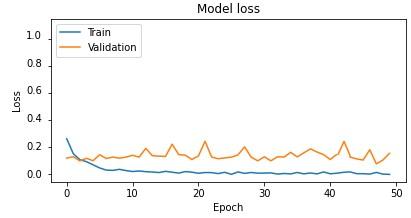
Figure 10 shows the performance graph of the training/test losses and accuracies of the DenseNet121 architecture for the 19,200 sampled training dataset. It was observed that the proposed model attained significant accuracy and loss values even in the 50th epoch.
(a) Training and testing accuracy analysis
(b) Training and testing loss analysis
Figure 10. Training and validation analysis over 50 epochs
Gender prediction is a critical and necessary process in forensic identification. Forensic experts and medical specialists employ traditional methods for gender estimation after years of training and education. In this study we proposed the DenseNet121 model using a deep transfer learning network and a fully automated technique to process panoramic dental x-ray images. The structural flexibility of the DenseNet121 architecture and the use of lesser parameters resulted in high-speed execution of training and verification processes. The weighted loss function was employed to eliminate the imbalance in gender classification, and the combination of early stopping and transfer learning was used to prevent over-learning. The best performance was achieved for the 4,800 test datasets with a classification accuracy of 97.25%. The proposed model, along with Grad-CAM based analysis also revealed that the mandible circumference and teeth are the most significant areas to consider in gender classification.
[1] Ozdemir, C., Gedik, M.A., Kaya, Y. (2021). Age estimation from left-hand radiographs with deep learning methods. Traitement du Signal, 38(6): 1565-1574. https://doi.org/10.18280/ts.380601
[2] Yetis, A.D., Yesilnacar, M.I., Atas, M. (2021). A machine learning approach to dental fluorosis classification. Arabian Journal of Geosciences, 14(2): 1-12. https://doi.org/10.1007/s12517-020-06342-2
[3] Ataş, M., Doğan, Y., Ataş, İ. (2016). Fast weighing of pistachio nuts by vibration sensor array. International Journal of Electronics and Electrical Engineering, 4(4): 313-317. https://doi.org/10.18178/ijeee.4.4.313-317
[4] Özdemi̇r, C., Ataş, M., Özer, A.B. (2013). Classification of Turkish spam e-mails with artificial immune system. 21st Signal Processing and Communications Applications Conference (SIU), IEEE. https://doi.org/10.1109/SIU.2013.6531457
[5] Dogan, Y., Keles, H.Y. (2022) Iterative facial image inpainting based on an encoder-generator architecture. Neural Comput & Applic., 34: 10001-10021. https://doi.org/10.1007/s00521-022-06987-y
[6] Ataṣ, M., Tekeli, A.E., Dönmez, S., Fouli, H. (2016). Use of interactive multisensor snow and ice mapping system snow cover maps (IMS) and artificial neural networks for simulating river discharges in Eastern Turkey. Arabian Journal of Geosciences, 9(2):1-17. https://doi.org/10.1007/s12517-015-2074-2
[7] Milošević, D., Vodanović, M., Galić, I., Subašić, M. (2019). Estimating biological gender from panoramic dental X-ray images. 11th International Symposium on Image and Signal Processing and Analysis (ISPA). https://doi.org/10.1109/ISPA.2019.8868804
[8] INTERPOL Disaster Victim Identifcation Guide. (2014).
[9] Jardin, P., Ponsaillé, J., Alunni-Perret, V., Quatrehomme, G. (2009). A comparison between neural network and other metric methods to determine sex from the upper femur in a modern French population. Forensic Sci. Int. 192(1-3): 127.e1-127.e6. https://doi.org/10.1016/j.forsciint.2009.07.014
[10] Badran, D.H., Othman, D.A., Thnaibat, H.W., Amin, W.M. (2015). Predictive accuracy of mandibular ramus flexure as a morphologic indicator of sex dimorphism in Jordanians. Int. J. Morphol., 33(4): 1248-1254. http://dx.doi.org/10.4067/S0717-95022015000400009
[11] Lin, C., Jiao, B., Liu, S., Guan, F., Chuang, N., Han, S., Lee, U. (2014). Sex determination from the mandibular ramus flexure of Koreans by discrimination function analysis using three-dimensional mandible models. Forensic Sci. Int., 236(191): 191-196. https://doi.org/10.1016/j.forsciint.2013.12.015
[12] Kim, D.I., Kim, Y.S., Lee, U.Y., Han, S.H. (2013). Sex determination from calcaneus in Korean using discriminant analysis. Forensic Sci. Int., 228(1-3): 177.e1-177.e7. https://doi.org/10.1016/j.forsciint.2013.03.012
[13] Akhlaghi, M., Bakhtavar, K., Bakhshandeh, H., Mokhtari, T., Farahani, M.V., Parsa, V.A., Mehdizadeh, F., Sadeghian, M.H. (2017). Sex determination based on radiographic examination of metatarsal bones in Iranian population. Int. J. Med. Toxicol. Forensic Med., 7(4): 203-208. http://dx.doi.org/10.22037/ijmtfm.v7i4
[14] Mahfouz, M., Badawi, A., Merkl, B., Abdel Fatah, E.E., Pritchard, E., Kesler, K., Moore, M., Jantz, R., Jantz, L. (2007). Patella sex determination by 3D statistical shape models and nonlinear classifiers. Forensic Sci. Int., 173(2-3): 161-170. https://doi.org/10.1016/j.forsciint.2007.02.024
[15] Gapert, R., Black, S., Last, J. (2009). Sex determination from the occipital condyle: Discriminant function analysis in an eighteenth and nineteenth century British sample. Am. J. Phys. Anthropol., 138(4): 384-394. https://doi.org/10.1002/ajpa.20946
[16] El Morsi, D.A., Al Hawary, A.A. (2013). Sex determination by the length of metacarpals and phalanges: X-ray study on Egyptian population. J. Forensic Leg. Med., 20(1): 6-13. https://doi.org/10.1016/j.jflm.2012.04.020
[17] Oner, Z., Turan, M.K., Oner, S., Secgin, Y., Sahin, B. (2019). Sex estimation using sternum part lenghts by means of artificial neural networks. Forensic Sci. Int., 301: 6-11. https://doi.org/10.1016/j.forsciint.2019.05.011
[18] Toy, S., Secgin, Y., Oner, Z., Turan, M.K., Oner, S., Senol, D. (2022). A study on sex estimation by using machine learning algorithms with parameters obtained from computerized tomography images of the cranium. Nature, 12: 4278. https://doi.org/10.1038/s41598-022-07415-w
[19] Hu, K.S., Koh, K.S., Han, S.H., Shin, K.J., Kim, H.J. (2006). Gender determination using nonmetric characteristics of the mandible in Koreans. J. Forensic. Sci., 51(6): 1376-1382. https://doi.org/10.1111/j.1556-4029.2006.00270.x
[20] Srivastava, P.C. (2010). Correlation of odontometric measures in Gender determination. Indian Acad Forensic Med., 32(1): 56-61.
[21] Ilić, I., Vodanović, M., Subašić, M. (2019). Gender estimation from panoramic dental X-ray images using deep convolutional networks. IEEE EUROCON 2019 -18th International Conference on Smart Technologies. https://doi.org/10.1109/EUROCON.2019.8861726
[22] Iscan, M., Kennedy, K. (1989). Reconstruction of Life from the Skeleton. Wiley-Liss.
[23] Lai, Y., Fan F., Wu.Q., Ke, W., Liao P. et al. (2021). LCANet: Learnable connected attention network for human identification using dental images. IEEE Transactions on Medical Imaging, 40(2): 905-915. https://doi.org/10.1109/TMI.2020.3041452
[24] Chen, H., Jain, A.K. (2004). Tooth contour extraction for matching dental radiographs. 17th International Conference on Pattern Recognition, Cambridge, UK, pp. 522-525. https://doi.org/10.1109/ICPR.2004.1334581
[25] Balci, Y., Yavuz, M.F., Cağdir, S. (2005). Predictive accuracy of sexing the mandible by ramus flexure. HOMO, 55(3): 229-237. https://doi.org/10.1016/j.jchb.2004.07.006
[26] Krogman, W.M. (1955). The human skeleton in forensic medicine. Postgrad Med., 17(2): A-48.
[27] de Oliveira Gamba, T., Alves, M.C., Haiter, N.F. (2016). Mandibular sexual dimorphism analysis in CBCT scans. Journal of Forensic and Legal Medicine, 38: 106-110. https://doi.org/10.1016/j.jflm.2015.11.024
[28] Vishwakarma, N., Guha, R. (2011). A study of sexual dimorphism in permanent mandibular canines and its implications in forensic investigations. Nepal Med Coll J., 13(2): 96-99.
[29] Maloth, K.N., Kundoor, V.K.R., Vishnumolakala, S.S.L.P., Kesidi, S., Lakshmi, M.V., Thakur, M. (2017). Mandibular ramus: A predictor for sex determination-A digital radiographic study. Journal of Indian Academy of Oral Medicine and Radiology, 29(3): 242-246. https://doi.org/10.4103/jiaomr.JIAOMR_170_16
[30] Loth, S.R., Henneberg, M. (1996). Mandibular ramus flexure: A new morphologic indicator of sexual dimorphism in the human skeleton. Am. J. Phys. Anthropol., 99(3): 473-485. https://doi.org/10.1002/(SICI)1096-8644(199603)99:3<473::AID-AJPA8>3.0.CO;2-X
[31] Loth, S.R., Henneberg, M. (1997). Ramus flexure and symphyseal base shape: sexually dimorphic morphology in the premodern hominid mandible. Am. J. Phys. Anthrop. Suppl., 24: 157-158.
[32] Loth, S.R., Henneberg, M. (1998). Mandibular ramus flexure is a good indicator of sexual dimorphism. Am. J. Phys. Anthropol., 105(1): 91-92. https://doi.org/10.1002/(SICI)1096-8644(199801)105:1<91::AID-AJPA9>3.0.CO;2-G
[33] Loth, S.R., Henneberg, M. (2000). Gonial iversion: Facial architecture, not sex. Homo, 51(1): 81-89.
[34] Deana, N.F., Alves, N. (2017). Nonmetrical sexual dimorphism in mandibles of Brazilian individuals. Biomed. Res. (India), 28(9): 4233-4238.
[35] Nagaraj, L.J., Gogula, S., Ghouse, N., Nigam, H., Sumana, C.K. (2017). Sex determination by using mandibular ramus: A digital radiographic study. Journal of Medicine, Radiology, Pathology and Surgery, 4: 5-8. https://doi.org/10.15713/ins.jmrps.99
[36] Ke, W., Fan, F., Liao, P., Lai, Y., Wu, Q., Du, W., Chen, H., Deng, Z., Zhang, Y. (2020). Biological gender estimation from panoramic dental X ray images based on multiple feature fusion model. Sensing and Imaging, 21: 54. https://doi.org/10.1007/s11220-020-00320-4
[37] Ortiza, A.G., Costab, C., Silvac, R.H.A., Biazevica, M.G.H., Michel-Crosatoa, E. (2020). Sex estimation: Anatomical references on panoramic radiographs using Machine Learning. Forensic Imaging, 20: 200-356. https://doi.org/10.1016/j.fri.2020.200356
[38] Kumar, A., Bhadauria, H.S., Singh, A. (2021). Descriptive analysis of dental X-ray images using various practical methods: A review. PeerJ Computer Science, 7: e620. https://doi.org/10.7717/peerj-cs.620
[39] Patanachai, N., Covavisaruch, N., Sinthanayothin, C. (2010). Wavelet transformation for dental X-ray radiographs segmentation technique. Eighth International Conference on ICT and Knowledge Engineering, pp. 103-106. https://doi.org/10.1109/ICTKE.2010.5692904
[40] Frejlichowski, D., Wanat, R. (2011). Automatic segmentation of digital orthopantomograms for forensic human identification. In: Maino, G., Foresti, G.L. (eds) Image Analysis and Processing – ICIAP 2011. ICIAP 2011. Lecture Notes in Computer Science, vol 6979. Springer, Berlin, Heidelberg. https://doi.org/10.1007/978-3-642-24088-1_31
[41] Pushparaj, V., Gurunathan, U., Arumugam, B. (2013). An effective dental shape extraction algorithm using contour information and matching by mahalanobis distance. Journal of Digital Imaging, 26(2): 259268. https://doi.org/10.1007/s10278-012-9492-4
[42] Lira, P.H.M., Giraldi, G.A., Neves, L.A.P., Feijoo, R.A. (2014). Dental R-ray image segmentation using texture recognition. IEEE Latin America Transactions, 12(4): 694-698. https://doi.org/10.1109/TLA.2014.6868871
[43] Abdi, A.H, Kasaei, S., Mehdizadeh, M. (2015). Automatic segmentation of mandible in panoramic X-ray. Journal of Medical Imaging, 2(4): 044003. https://doi.org/10.1117/1.JMI.2.4.044003
[44] Poonsri, A., Aimjirakul, N., Charoenpong, T., Sukjamsri, C. (2016). Teeth segmentation from dental x-ray image by template matching. 9th Biomedical Engineering International Conference (BMEiCON), pp. 1-4. https://doi.org/10.1109/BMEiCON.2016.7859599
[45] Zak, J., Korzynska, A., Roszkowiak, L., Siemion, K., Walerzak, S., Walerzak, M., Walerzak, K. (2017). The method of teeth region detection in panoramic dental radiographs. In: Kurzynski, M., Wozniak, M., Burduk, R. (eds) Proceedings of the 10th International Conference on Computer Recognition Systems CORES 2017. CORES 2017. Advances in Intelligent Systems and Computing, vol. 578. Springer, Cham. https://doi.org/10.1007/978-3-319-59162-9_31
[46] Mahdi, F.P., Kobashi, S. (2018). Quantum particle swarm optimization for multilevel thresholding-based image segmentation on dental X-ray images. Joint 10th International Conference on Soft Computing and Intelligent Systems (SCIS) and 19th International Symposium on Advanced Intelligent Systems (ISIS), pp. 1148-1153. https://doi.org/10.1109/SCIS-ISIS.2018.00181
[47] Fariza, A., Arifin, A.Z., Astuti, E.R., Kurita, T. (2019). Segmenting tooth components in dental X-ray images using Gaussian kernel-based conditional spatial Fuzzy C-Means clustering algorithm. International Journal of Intelligent Engineering and Systems, 12(3): 108-117. https://doi.org/10.22266/ijies2019.0630.12
[48] Aliaga, I., Vera, V., Vera, M., García, E., Pedrera, M., Pajares, G. (2020). Automatic computation of mandibular indices in dental panoramic radiographs for early osteoporosis detection. Artificial Intelligence in Medicine, 103: 101816. https://doi.org/10.1016/j.artmed.2020.101816
[49] Esmaeilyfard, R., Paknahad, M., Dokohaki, S. (2020). Sex classification of first molar teeth in cone beam computed tomography images using data mining. Forensic Science International, 318: 110633. https://doi.org/10.1016/j.forsciint.2020.110633
[50] Oktay, A.B. (2017). Tooth detection with convolutional neural networks. Medical Technologies National Congress (TIPTEKNO), pp. 1-4. https://doi.org/10.1109/TIPTEKNO.2017.8238075
[51] Chu, P., Bo, C., Liang, X., Yang, J., Megalooikonomou, V., Yang, F., Huang, B., Li, X., Ling, H. (2018). Using octuplet Siamese network for osteoporosis analysis on dental panoramic radiographs. 40th Annual International Conference of the IEEE Engineering in Medicine and Biology Society (EMBC), pp. 2579-2582. https://doi.org/10.1109/EMBC.2018.8512755
[52] Lee, J.H., Han, S.S., Kim, Y.H., Lee, C., Kim, I. (2019). Application of a fully deep convolutional neural network to the automation of tooth segmentation on panoramic radiographs. Oral Surgery, Oral Medicine, Oral Pathology and Oral Radiology, 129(6): 635-642. https://doi.org/10.1016/j.oooo.2019.11.007
[53] Muramatsu, C., Morishita, T., Takahashi, R., Hayashi, T., Nishiyama, W., Ariji, Y., Zhou, X., Hara, T., Katsumata, A., Ariji, E., Fujita, H. (2020). Tooth detection and classification on panoramic radiographs for automatic dental chart filing: Improved classification by multi-sized input data. Oral Radiology, 37: 13-19. https://doi.org/10.1007/s11282-019-00418-w
[54] Simonyan, K., Zisserman, A. (2014). Very deep convolutional networks for large-scale image recognition. arXiv:1409.1556 [cs]. arXiv: 1409.1556.
[55] He, K., Zhang, X., Ren, S., Sun, J. (2015). Deep residual learning for image recognition. arXiv, arXiv:1512.03385.
[56] Tan, M., Le, Q. (2019). EfficientNet: Rethinking model scaling for convolutional neural networks. In International Conference on Machine Learning, pp. 6105-6114.
[57] Huang, G., Liu, Z., Van Der Maaten, L., Weinberger, K.Q. (2017). Densely connected convolutional networks. Proceedings of the IEEE Conference on Computer Vision and Pattern Recognition, pp. 4700-4708. https://doi.org/10.1109/CVPR.2017.243
[58] Ataş, M. (2016). Open Cezeri Library: A novel Java based matrix and computer vision framework. Computer Applications in Engineering Education, 24(5): 736-743. https://doi.org/10.1002/cae.21745
[59] Kandel, I., Castelli, M., Popovic, A. (2020). Comparative study of first order optimizers for image classification using convolutional neural networks on histopathology images. J. Imaging, 6(9): 92. https://doi.org/10.3390/jimaging6090092
[60] Ketkar, N. (2017). Stochastic gradient descent. In: Deep Learning with Python. Apress, Berkeley, CA. https://doi.org/10.1007/978-1-4842-2766-4_8
[61] Tieleman, T., Hinton, G. (2012), Lecture 6.5 RmsProp: divide the gradient by a running average of its recent magnitude. COURSERA: Neural Networks for Machine Learning. https://www.cs.toronto.edu/~hinton/coursera/lecture6/lec6.pdf.
[62] Stone, M. (1974). Cross-validatory choice and assessment of statistical predictions. J. R. Stat. Soc. Ser. B Methodol.m 36(2): 111-133. https://doi.org/10.1111/j.2517-6161.1974.tb00994.x
[63] Google Colab. https://colab.research.google.com/, accessed on 8 April 2022.
[64] Sokolova, M., Japkowicz, N., Szpakowicz, S. (2006). Beyond accuracy, F-score and ROC: A family of discriminant measures for performance evaluation. In: Sattar, A., Kang, Bh. (eds) AI 2006: Advances in Artificial Intelligence. AI 2006. Lecture Notes in Computer Science, vol. 4304. Springer, Berlin, Heidelberg. https://doi.org/10.1007/11941439_114
[65] Liu, C., White, M., Newell, G. (2011). Measuring and comparing the accuracy of species distribution models with presence–absence data. Ecography, 34(2): 232-243. https://doi.org/10.1111/j.1600-0587.2010.06354.x
[66] Selvaraju, R.R., Cogswell, M., Das, A, Vedantam, R., Parikh, D., Batra D. (2017). Grad-CAM: Visual explanations from deep networks via gradient-based localization. IEEE International Conference on Computer Vision, Venice, Italy, pp. 618-626. https://doi.org/10.1109/ICCV.2017.74
[67] Steyn, M., İşcan, M.Y. (2008). Metric sex determination from the pelvis in modern Greeks. Forensic Sci. Int., 179(1): 86.e1-86.e6. https://doi.org/10.1016/j.forsciint.2008.04.022
[68] Jardin, P., Ponsaillé, J., Alunni-Perret, V. Quatrehomme, G. (2009). A comparison between neural network and other metric methods to determine sex from the upper femur in a modern French population. Forensic Sci. Int. 192(1-3): 127.e1-127e6. https://doi.org/10.1016/j.forsciint.2009.07.014
[69] Saini, V., Srivastava, R., Rai, R.K. (2011). Mandibular ramus: An indicator for sex in fragmentary mandible. Journal of Forensic Sciences, 56(1): 13-16. https://doi.org/10.1111/j.1556-4029.2010.01599.x
[70] Indira, A.P., Markande, A., David, M.P. (2012). Mandibular ramus: An indicator for sex determination - A digital radiographic study. Journal of Forensic Dental Sciences, 4(2): 58-62. https://doi.org/10.4103/0975-1475.109885
[71] Alias, A., Ibrahim, A., Abu Bakar, S., Shafie, M.S. (2018). Anthropometric analysis of mandible: An important step for sex determination. La Clinica Terapeutica, 169(5): 217-223. https://doi.org/10.7417/CT.2018.2082
[72] Blanco, N.V., Vilas, R.R., Carreira, M.J., Carmona, I.T. (2020). Towards deep learning reliable gender estimation from dental panoramic radiographs. 9th European Starting AI Researchers’ Symposium (STAIRS) co-located with 24th European Conference on Artificial Intelligence (ECAI 2020).
[73] Mualla, N., Houssein, E., Hassan, M.R. (2020). Dental age estimation based on X-ray images. CMC-Computers, Materials & Continua, 62(2): 591-605. https://doi.org/10.32604/cmc.2020.08580
[74] Rajee, M.V., Mythilib, C. (2021). Gender classification on digital dental x-ray images using deep convolutional neural network. Biomedical Signal Processing and Control, 69: 102939. https://doi.org/10.1016/j.bspc.2021.102939
[75] Nithya, L., Sornam, M. (2021). Deep convolutional networks in gender classification using dental X-ray images. In: Chandramohan, S., Venkatesh, B., Sekhar Dash, S., Das, S., Sharmeela, C. (eds) Artificial Intelligence and Evolutionary Computations in Engineering Systems. Advances in Intelligent Systems and Computing, vol. 1361. Springer, Singapore. https://doi.org/10.1007/978-981-16-2674-6_29
[76] Santosh, K.C., Nijalingappa, P., Vikas, G., Raju, R., Ekta, P., Piyush, K.S., Stephen, J.N. (2022). Machine learning techniques for human age and gender identification based on teeth X-ray images. J Healthc Eng., 2022: 8302674. https://doi.org/10.1155/2022/8302674
[77] Vila-Blanco, N., Carreira, M.J., Varas, Q.P., Balsa, C.C., Tomás, I. (2020). Deep neural networks for chronological age estimation from OPG images. IEEE Trans. Medical Imaging, 39(7): 2374-2384. https://doi.org/10.1109/TMI.2020.2968765