Yanming Zhao | Guoan Su* | Hong Yang | Tianshuai Zhao | Songwen Jin | Jianing Yang
© 2022 IIETA. This article is published by IIETA and is licensed under the CC BY 4.0 license (http://creativecommons.org/licenses/by/4.0/).
OPEN ACCESS
The graph convolution algorithm currently suffers from the drawback of not fusing point cloud information and point cloud topology structure information based on visual selectivity features and using absolute quantities like distance as features, resulting in the algorithm losing geometric invariance. This information serves as the foundation for the "Graph Convolution Algorithm Based on Visual Selectivity and Application of Point Cloud Analysis". In order to propose a graph convolutional kernel and its design method based on visual selectivity, the algorithm analyzes the global characteristics of the point cloud "close in the vicinity and sparse in the distance," the local selectivity of the point cloud topology structure in the neighborhood, and the consistency between features and visual selectivity of primates. By combining point cloud information with point cloud topology structure information features, a graph convolution computation method was built, and the algorithm's geometric invariance was confirmed. The recognition and semantic segmentation performances of the approach in this study were verified using the ModelNet40 and ShapeNetPart data sets in comparison to the PointNet, PointNet++, DGCNN, KPConv, and 3D-GCN algorithms. The experimental design demonstrates that the algorithm presented in this research is accurate and practical, has geometric invariance, and performs better at semantic segmentation and recognition than conventional algorithms.
visual computing, visual selectivity, graph convolution analysis, receptive field, point cloud topology, support set
3D point cloud data is now easier to collect thanks to advances in RGBD and LIDAR sensor technology. This has led to the current research hotspot of 3D point cloud data processing technology, which is widely used in augmented reality, unmanned aerial vehicles, and automatic driving, among other things [1-3], and has produced positive research and application results.
Recent literature reviews demonstrate that point cloud data exhibits the characteristics of disorder, lack of organization, closeness in the immediate area, and sparsity in the distance. Due to the grid structure of 2D spatial data, which determines the topological relationship of 2D spatial data, traditional convolution technology can handle 2D spatial data effectively. Point cloud data, on the other hand, has unstructured properties, meaning that it is unclear how geographical data is related topologically. Therefore, point cloud data cannot be processed using conventional convolution algorithms. Unstructured data cannot be used for convolution calculations. Researchers use both indirect and direct data processing techniques to realize point cloud data processing and analysis, with the graph convolution algorithm standing out as a key research technique.
The indirect method is to transform the unstructured point cloud data into spatial data with a grid structure by creating a spatial grid method, and on this basis realize the traditional convolution and its improved various operations. This approach is motivated by the inherent domain relationship determined by the two-dimensional spatial data grid. Voxel filtering methods [4-6] and multi-view approaches [7-9] are some of its key techniques.
The voxel filtering method registers the unstructured point cloud data as a volume with a three-dimensional spatial grid structure using the spatial transformation and spatial sampling technology of creating a three-dimensional spatial grid, which is motivated by the inherent domain relationship determined by the two-dimensional spatial data grid. The traditional convolution calculation is carried out on the voxel filter data set, and the voxel filter data is directly sampled from the voxel filter data or the sensor. In many fields, this methodology has produced positive research and application results. The voxel filtering approach, however, also has issues with inadequate resolution brought on by registration and sampling, as well as excessive storage capacity brought on by excessive data storage redundancy. The OCTREE approach [5, 6] has been presented as a solution to this issue, although the impact is not particularly noticeable. The primary issue is that there is an excessive amount of human involvement in the sampling and registration processes, which obliterates the point cloud's underlying spatial organization.
The multi-view method realizes the conversion and dimensionality reduction of the two-dimensional sequence of point cloud data before applying the conventional convolution operation to the 2D view sequence successively to realize point cloud data processing. The multi-view method uses the 3D research object as the center and the fixed viewing distance r as the radius, collecting the two-dimensional data views of the research object from various perspectives to produce the research view sequence. However, there are furthermore the following three issues: (1) In the process of 2D serialization and dimensionality reduction, the multi-view technique loses the spatial topology information of the point cloud data; (2) It is challenging to reconstruct 3D data. (3) It is impossible to realize scene segmentation. These are essential for processing, analyzing, and using point cloud data.
In order to make traditional convolution processes easier, the primary idea behind voxel filtering and multi-view approaches is to convert unstructured data into structured data using gridding or multi-view spatial dimensionality reduction [9, 10]. In contrast, the multi-view method gathers point cloud data through multi-angle views, converting point cloud data into a dimensionality reduction representation of a two-dimensional grid data sequence. The difference is that the voxel filtering method uses sampling to register the point cloud data into a three-dimensional grid, realizing the structured expression of point cloud data through the neighborhood grid technology of Euclidean space. Therefore, datasets produced by voxel filtering and multi-view processing can be processed routinely using classic convolution procedures.
Gridding data, however, weakens both the topological selectivity and the spatial topological link of the point cloud data from many perspectives. The term "topological selectivity" refers to the qualitatively measurable direction selectivity of the point cloud data distribution as well as the probability certainty of the strength of the distribution. This topological selectivity, which can be completely stated under the condition of adequate sampling, can be referred to as the topological selectivity of point cloud data. This property is invariant in geometry. Therefore, the direct data processing approach will successfully address the aforementioned shortcomings.
The direct data processing technique involves immediately applying the graph convolution analysis approach to the 3D point cloud data without first subjecting it to voxel filtering or multi-view conversion. The two most crucial deep learning techniques are PointNet [11], PointNet++ [12], and their enhanced algorithms that followed [13-20].
For the disorganized, unstructured, densely packed but sparsely distributed properties of point cloud data. The T-net method, point-by-point multi-layer perceptron, and channel-by-channel maximum pooling method are used by PointNet [11] to learn the general properties of 3D point cloud data and to address the issue of disorder in this data. The algorithm itself has the flaw of being unable to determine what the local attributes of the point cloud are. In order to achieve data sampling at various scales and resolutions and apply it to the sampled point cloud PointNet algorithm, which extracts the local feature extraction of the sampled point cloud, the PointNet++ [12] algorithm uses two processing methods, Multi scale grouping (MSG) and Multi resolution grouping (MRG). The issue of the PointNet algorithm ignoring local features has been partially resolved. To increase the application potential of this kind of algorithm, the follow-up algorithms are continuously improved in the acquisition of global features, local features, and invariant features.
The aforementioned approach, meanwhile, overlooks the 3D point cloud data's spatial topology structure, which has a considerable graph structure and can be represented by a graph. As a result, a new study area for 3D point clouds has emerged: graph convolution analysis method based on graph structure. Good research and application development has been made in this area. This approach, which is based on the PointNet++ algorithm, can extract the local spatial properties of a collection of point clouds from their spatial subset. The DGCNN technique [21] constructs a local graph structure by first determining the closest neighbors of 3D points in the feature space, then performing an edge convolution operation to extract features. The aforementioned concepts were expanded upon by Shen et al. [21], who also discovered additional spatial topological data while aggregating features. The neighborhood node features used by RS-CNN [22] are weighted sums, where each weight is learned using an MLP based on the geometric relationship between two points. These studies try to understand the local topological characteristics of 3D point clouds [23].
Although the aforementioned techniques have made significant advancements in application and good research development in graph representation and graph convolution, the following issues still exist: (1) The use of the point cloud's spatial topology as two distinct aspects It results in imperfect feature learning in various algorithms as opposed to applying both to the same algorithm. (2) The algorithm lacks neurophysiological evidence to demonstrate its theoretical viability. (3) The close in proximity and sparse in distance features of the point cloud data are not combined, and a topological selectivity calculation rule is created by combining it with primate visual selectivity. (4) The algorithm uses the actual coordinates of the point or the distance vector as the input feature, which results in the model b not having rotation, stretching and deformation.
Graph Convolution Algorithm Based on Visual Selectivity and Application of Point Cloud Analysis was subsequently proposed in light of this. This algorithm's primary innovations are as follows: (1) Inspired by the theory of visual selectivity, a graph convolutional kernel and its construction method based on visual selectivity are proposed; this method combines visual selectivity, close in the proximity and sparse in the distance features of point clouds, and point cloud topology structure selectivity; it also effectively extracts point cloud spatial topology selectivity features, solves the geophysical problem, and uses probability calculation method and weight normalization method. (2) To learn the spatial features of the point cloud elements, a spatial convolution method based on the graph convolutional kernel is created and combined with the theory of visual selectivity. (3) Create a depth map convolutional neural network using the convolution computation, then use it to handle 3D point clouds. (4) Create the point set's minimal generation subset and minimal support structure, then create a graph that expresses all of the point cloud's selected properties.
The design of the graph convolution kernel and the design of the convolution calculation method are the two fundamental components of the graph convolution algorithm based on visual selectivity.
The near in proximity and sparse in distance elements of the point cloud, as well as the structural selectivity of the point cloud topology, are all congruent with the visual selectivity of primates. The distribution of the receptive field in the visual space of primates follows the visual selectivity trait of "close in the vicinity and sparse in the distance."
As a result, 3D point cloud data has similar characteristics and robust visual basis functions in the visual space. In contrast to the visual basis functions with different functions, which exist in regions far apart and form a relatively slow-changing structure, the visual basis functions with different functions exist in a fixed spatial region and have a consistent spatial topology structure. The point cloud data is a collection of point sets with stable spatial information and a spatial topology structure, which in turn has a significant data redundancy row.
As a result, the point cloud based on visual selectivity need to have the qualities listed below:
(1) The global point cloud space is made up of a number of point cloud subspaces, and its spatial topology is stable and consistent.
(2) Each point cloud subspace in the global space has a separate basis function (receptive field) and a topology that is either constant or slowly evolving. These properties can be calculated using probabilistic methods.
(3) Each independent subspace has modest topological structure change, spatial independence, and functional resemblance to visual basis functions; Each point subset in the independent space has comparable visual functions, comparable visual basis functions, and gradually changing visual space topology.
(4) Each point cloud space's qualities have statistical properties. Through statistical analysis, the lack of data collection-related spatial completeness is resolved, and the collection set can be increased through visually consistent selection.
(5) Each point cloud subset has a minimum generation structure, which can represent any point or structure within the subset. This structure is made up of the minimum generation point set and its spatial support structure.
2.1 Convolution kernel design
Based on the above theoretical analysis, the convolutional kernel $filter_p^r$ (receptive field of point p) of point p in the 3D point cloud space can be defined as:
$filter_p^r=\left\{M_p^r, e d g e_p^r\right\}$ (1)
where, $M_p^r$ is the point p and the points of its point cloud space with the radius of r; $e d g e_p^r$ is the set of edges between the points in set $M_p^r$ and point p, i.e., the effective visual topology of point p. The set has the following features:
(1) Set $filter_p^r$ is a finite set, i.e., sets $M_p^r$ and $e d g e_p^r$ are both finite and have redundancy.
(2) Since $filter_p^r$ is a finite redundant set, there exists at least one minimum support set ${hold\text_filter }_p^r=\left\{\bar{M}_p^r, \overline{ { edge }}_p^r\right\} \subset filter _p^r$, where $\bar{M}_p^r \subset M_p^r$, $\overline{e d g e}_p^r \subset e d g e_p^r, \forall e \in \overline{e d g e}_p^r$ and $e \neq 0$. Thus, in the point cloud, ${hold\text_filter }_p^r$ expresses the topological information and the topological selectivity of the point cloud area with p as the circle center and r as the radius.
(3) ${hold\text_filter }_p^r$ is not unique.
(4) Inspired by visual selectivity, ${hold\text_filter }_p^r$ is an acquirable and illustrative quantity after training.
(5) Any point or edge in ${filter }_p^r$ can be expressed by the point or edge of ${hold\text_filter }_p^r$.
(6) Depending on the values of hyperparameter r, the support features of point p on different scales can be obtained, and the selective features of the global and local point cloud structures of that point can be obtained: $Global\text_faeture \subset hold \text_filter { }_p^r$ and $local \quad feature \subset hold \text_filter { }_p^r$.
(7) Maximum pooling convolution: When $\forall r \in R$, $\left\{\right. hold \left._{ {filter }_p^r}\right\}$ is the set of kernels at different scales r, $\forall p \in \bar{M}_p^r$. Then, the maximum pooling convolution z of point p can be expressed as:
Max_Pool_layer(q,hold_filterpr)= $\max _r$(convolutioncoff($p$, hold $_{\text {filter }_p^r}$)) (2)
In the algorithm, the layer formed according to this formula is called the maximum pooling layer, which realizes feature aggregation at different scales.
Based on the above analysis, inspired by the theory of primate visual selectivity, combined with the distribution of points in the point cloud in space, the convolution kernel of the point cloud (point cloud space receptive field with p as the center and radius r) can be defined for:
hold_filter ${ }_p^r=\left\{\bar{M}_p^r, \overline{e d g e}_p^r\right\}=\left\{p_m, p_n \mid p_m \in \mathrm{N}\left(p_n, r\right)\right\}=\left(r, \theta, d_\theta, n_\theta, w_\theta,(x, y, z)\right)$ (3)
Here, the parameter is the super parameter of the basis function, which determines the observation space range of the receptive field, determines the size of the receptive field and the scale of the observation direction, and is a decisive factor; the parameter θ represents the observation direction in the r neighborhood, indicating that the basis function points in the direction are relatively dense; the parameter $d_\theta$ indicates that in the direction θ, the point cloud space topology selectivity strength is related to the number of point clouds in the direction and the distance between the point $p_n$ and the geometric center of the point in the area; the parameter $n_\theta$ indicates that in the direction In the upper r range, the number of receptive field basis functions is a concentrated expression of visual selectivity; the parameter $w_\theta$ indicates the update degree of the direction range after each training within the r range in the direction. Parameters: represented as the spatial position information of point $p_m$ position.
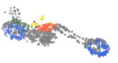
In the neighborhood of r, the convolution kernel design method of point P is show in Figure 1.
Figure 1. The design process diagram of the convolution kernel
Step 1. KNN clustering is adopted to divide hold_filter ${ }_p^r$ into K subsets:
hold_filter ${ }_p^r=\bigcup_{q=1}^K$ hold_filter $_p^r(q)$ (4)
Step 2. Compute the geometric center center(q) of each subset ${{hold_{filter}}_p^r}(q)$:
$\operatorname{center}(q)=\left(x_q, y_q, z_q\right)=\left(\frac{1}{T} \sum_{j=1}^T x_q^j, \frac{1}{T} \sum_{j=1}^T y_q^j, \frac{1}{T} \sum_{j=1}^T z_q^j\right)$ (5)
Step 3. Parameter learning:
$\theta=\left(\frac{\partial f}{\partial x}, \frac{\partial f}{\partial y}, \frac{\partial f}{\partial z}\right)=\left(\frac{p_m-p_n}{\left\|p_m-p_n\right\|}\right)$
$n_\theta=$ sizeof $\left(\right.$ hold_filter $\left.{ }_p^r(q)\right)$
$w_\theta^i=\frac{n_\theta^i}{n_\theta^{i-1}}$
$d_\theta^j=\frac{d_{(p, q)}^j \times n_\theta^j}{\sum_{j=1}^M d_{(p, q)}^j \times n_\theta^j} \times w_\theta^i$ (6)
Step 4. Forming convolutional kernels:
${hold_{ {filter }}}_p^r=\left(r, \theta^j, d_\theta^j, n_\theta^j, w_\theta^j, x, y, z\right)^r, j=1,2,3, \ldots, K$ (7)
where, $\theta^j, d_\theta^j, n_\theta^j, w_\theta^j, x, y$, and $z$ are learned through training
2.2 Graph convolution algorithm design
The graph convolution calculation is to calculate the direct similarity between the filter kernel and the analyzed point, therefore, the graph convolution calculation of point Q can be expressed as:
$convolution_{ {coff }}= similitude \left(\right.$ $\left.hold\text_filter_p^r, Q\right)+\operatorname{correct}\left(\right.$ $\left.hold\text_filter_p^r, Q\right)$ (8)
According to the requirements of similarity calculation in this paper, combined with the definition of vector inner product, the inner product of self-defined matrices A and B is defined as: if matrix A is expressed as $\alpha_i, i=1,2,3, \ldots, K_1$ by row vector, and matrix B as row vector $b_j, j=1,2,3, \ldots, K_2$, then the inner product is:
$A \odot B=\frac{1}{N} \sum_{\theta_i=\theta_j \text { and } \theta_i \neq \Phi, \text { and } \theta_j \neq \Phi} \quad a_i \odot b_j$ (9)
where, N represents the number of rows whose corresponding rows of matrices A and B are not zero vectors, and Φ represents an empty set. Therefore, similar calculations in graph convolution are expressed as:
similitude(hold_filter $\left.{ }_p^r, Q\right)=$ hold_filter ${ }_p^r \odot Q$ (10)
The modified part of the similarity calculation is expressed as:
$\operatorname{correct}\left(\right.$ hold_filter $\left.{ }_p^r, Q\right)=$
$\frac{1}{\max (\text { size }(\text { hold_filter }_p^r), \text { size }(Q))} \times$
jacard $($ hold_filterer $(\theta), Q(\theta))=$
$\frac{1}{\max (\operatorname{size}(\text { hold_filter }_p^r), \operatorname{size}(Q))} \times \frac{\text { hold_filter }(\theta) \cap Q(\theta)}{\text { hold_filter }(\theta) \cup Q(\theta)}$ (11)
where, correct $\left({{hold_{\text {filter}}}_p^r}, Q\right)$ is the matrix ${hold_{filter}}_p^r$. The modification of Q graph convolution increases the similarity of graph convolution. To sum up, the graph convolutional coefficient is:
convolution $_{\text {coff }}=$ hold_filter $_p^r \odot Q+$
$\frac{1}{\max (\operatorname{size}(\text { hold_filter } \quad _p^r), \quad \operatorname{size}(Q))} \times \frac{\text { hold_filter }(\theta) \cap Q(\theta)}{\text { hold_filter }(\theta) \cup Q(\theta)}$ (12)
Thus, 3D_RFGCN,3D receptive field graph convolution algorithm can be expressed as:
|
Input: Matrix hold_filterrp, and Q |
|
Proc: S1: Solve graph convolutional similarity by similitude (hold_filter $\left.{ }_p^r, Q\right)=$ hold_filter $_p^r \odot Q$ S2: Solve graph convolutional modification coefficient by correct $\left(\right.$ hold_filter $\left.{ }_p^r, Q\right)=$ $\frac{1}{\max \left(\text { size }\left(\text { hold_filter }{ }_p^r\right), \text { size }(Q)\right)} \times \frac{\text { hold_filter }(\theta) \cap Q(\theta)}{\text { hold_filter }(\theta) \cup Q(\theta)}$ S3: Solve graph convolutional coefficient by convolution $_{\text {coff }}=$ similitude $\left.{\text {(hold_filter }}{ }_p^r, Q\right)+$ correct $\left(\right.$ hold_filter $\left._p^r, Q\right)$ |
|
Output: Solve graph convolutional coefficient convolution $_{\text {coff }}$. |
2.3 Maximum pooling layer
Maximum pooling: When $\forall r \in R$, $\left\{\right.$ hold_filter $\left._p^r\right\}$ represents the set of kernels at different scales r, $\forall p \in \bar{M}_p^r$. Then, the maximum convolution $\mathrm{z}$ of point $\mathrm{p}$ is:
Max_Pool_layer $\left(q\right.$, hold_filter $\left.{ }_p^r\right)=$
$\max _r\left(\right.$ convolution $_{\text {coff }}\left(p\right.$, hold $\left.\left._{\text {filter }_p^r}\right)\right)$ (13)
In the algorithm, the layer formed according to this formula is called the maximum pooling layer, which realizes feature aggregation at different scales.
2.4 The overall structure of the algorithm
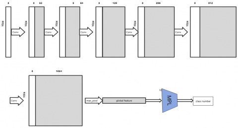
2.4.1 Classification algorithm design
In order to identify which known category the input 3D point cloud data s belongs to, the algorithm in this paper fuses the 3D_RFGCN layer and the Max_Pool_layer layer into one layer, and realizes the classification through a multi-layer perceptron (MLP). The standard soft_max loss function and gradient descent method are used for parameter learning of this algorithm. Therefore, the classification algorithm is designed as Figure 2:
Figure 2. Classification algorithm structure
2.4.2 Semantic segmentation algorithm design
The 3D point cloud data can be semantically segmented using the algorithm shown in this research. We propose a shared MLP method for point-by-point classification in order to accomplish this goal. The characteristics of 3D point cloud data between different layers do not match because the algorithm uses a pooling mechanism. Accordingly, this paper defines the following aggregation operations:
$p_{\bar{n}}^{j+1}=\operatorname{argmin}\left\{\left\|p-p_n^j\right\| \mid \forall p \in p^{j+1}\right\}$ (14)
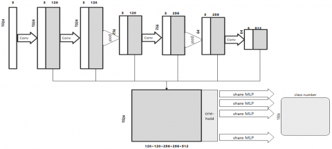
Therefore, the generated pooled features are 2, and the corresponding semantic segmentation network is as Figure 3.
Figure 3. Segmentation algorithm structure
2.4.3 Algorithm invariance
Although previous works like [14, 21, 23-30] report good geometric invariance performance, they typically take into account global coordinates or call for point cloud normalization to reduce this data variance, which will limit their immutability. Through the use of 3D convolution kernels, the text algorithm learns relative quantity features such as directional information and directional selectivity in the local receptive field. The formation of these features is independent of specific positions and distances, and the algorithm uses a pooling mechanism to further increase its geometric invariance. As a result, the algorithm presented in this paper demonstrates strong shift, scale, and rotation invariance.
3.1 Classification algorithm
3.1.1 Datasets
ModelNet40 dataset, which contains 40 categories with a total of 12311 models. According to the experimental needs of the classification algorithm, each category of the data set is divided into a training set and a test set according to 7:3, and the ratio of sample data is: training set:test set=8613:2698; and 1024 samples are resampled from each model Points form a new training and testing set.
3.1.2 Network parameter configuration
In the parameter setting of the three-dimensional graph convolutional neural network in this paper, the feature extraction is 5 layers, and the order of convolution kernels from the bottom layer to the top layer is (32, 64, 128, 256, 1024); the number of supports is S=1, , The number of domain nodes is M=32; the maximum pooling layer of the network is 3; the sampling rate is 4; the output result is a 1024-dimensional vector; the learning rate is 0.00001; batch_size=8; the optimization method is ADAM.
3.1.3 Experimental results
On the same data set, compare the classification performance of our algorithm with the traditional algorithms PointNet [12], PointNet++ [12], DGCNN [21], KPConv [24] and 3D-GCN [23]. The experimental results are shown in Table 1.
The data in the above table demonstrates that when numerous state-of-the-art methods are compared with the algorithm in this article, the algorithm in this paper has comparable or good performance when there is no geometric change in the test data.
A 3D point cloud dataset with 1024 sample points is created, and the point cloud data is standardized to a unit sphere with zero mean without data augmentation in order to assess the model's invariance. The geometric invariance of the algorithm in this study and the technique above is confirmed under the three conditions of translation, stretching, and rotation. The graphic displays the outcomes of the experiment:
Table 1. Classification performance comparison
|
Algorithm |
INPUT |
Point |
Acc(%) |
Algorithm |
INPUT |
Point |
Acc(%) |
|
ECC [29] |
xyz |
1K |
87.4 |
SO-Net [26] |
xyz |
2k |
90.9 |
|
PointNet [11] |
xyz |
1K |
89.2 |
KPConv [25] |
xyz |
6.8k |
92.9 |
|
Kd-Net(depth=10) [28] |
xyz |
1K |
90.6 |
PointNet++ [13] |
Xyz,normal |
5k |
91.9 |
|
PointNet++ [12] |
xyz |
1K |
90.7 |
So-Net [26] |
Xyz,normal |
5k |
93.4 |
|
KCNet [21] |
xyz |
1K |
91.0 |
3D-GCN [24] |
xyz |
1k |
92.1 |
|
MRTNet [27] |
xyz |
1K |
91.2 |
ours |
xyz |
1k |
94.9 |
|
DGCNN [20] |
xyz |
1K |
92.9 |
|
|
|
|
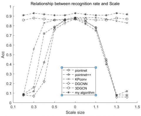
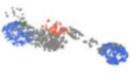
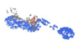
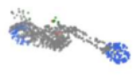
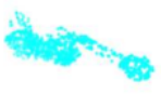
(a) Shift
(b) Scala
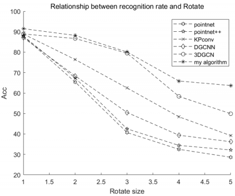
(c) Rotate
Figure 4. Evaluation of invariant properties on ModelNet40, (a) Parallel shift: Object moves randomly within distance (unshifted version denoted as 0) (b) Scale: Object scaled to a different size (original size denoted as 1), (c) Rotation: An object rotated in an upward direction (degrees are indicated in this figure).
Note that the DGCNN in [21] is pre-trained on objects with scaling variables (i.e., the scaling range is within [0.5, 1.5]), but it cannot handle scaling variables that are not shown as shown in (b).
The Figure 4 shows that extracting features from global coordinates causes PointNet and DGCNN to perform much worse with coordinate shift. The only model that can identify with sufficient performance given the scale variables is my algorithm, which performs better in terms of shape rotation invariance. The efficacy and robustness of the suggested approach are thus supported by the aforementioned experiments.
3.2 3D model segmentation algorithm
3.2.1 Datasets
The ShapeNetPart dataset [31] is used in this study as the verification database to assess the algorithm's capacity for 3D object segmentation. The collection consists of 16 different item categories represented by 16881 CAD models, with each object point corresponding to a part label. Each object type has access to 2 to 6 part categories, for a total of 50 categories. This experiment extracts 1024 points from each 3D model for training and testing to compare with conventional algorithms.
3.2.2 Method of evaluation
The mean intersection-over-union ratio (mIoU), which represents the average IoU for each part type in the object category, is used in this study to assess segmentation performance.
IoU, a notion utilized in target identification, is short for Intersection over Union. IoU determines the intersection and union ratio, or overlap rate, between "predicted boundary" and "actual border." The best scenario is total overlap, or a ratio of 1.
$\operatorname{IoU}\left(S_{\text {Predict }}, S_{\text {True }}\right)=\frac{S_{\text {Predict }} \quad \cap \quad S_{\text {True }}}{S_{\text {Predict }} \quad \cup \quad S_{\text {True }}}$ (15)
The average of the IoUd of all shape instances in the object category is known as the joint mean intersection (mIoU), and it is written as follows:
$m I o U=\frac{1}{N} \sum_{i=1}^N \operatorname{IoU}(i)$ (16)
where, N represents the number of instances in the object. In this experiment N=16.
3.2.3 Network parameter configuration
In Figure 3, the model architecture is displayed. The feature extraction portion is composed of two 3D Graph Max pooling layers with fixed sample rate r=6 and five layers with kernel numbers (128, 128, 256, 512) at pertinent layers. We set the neighbor number M=80 for the receptive field in 3D-GCN and the support number S=1 for each core. Features for segmentation are concatenated from layer outputs at various scales, as discussed in Section 2.3. We also have a one-hot vector indicating the object type related to the aforementioned features, which is then followed by three shared MLP layers to categorize the segmented labels for each point, as in PointNet [21]. We use the ADAM optimizer to train b our algorithm with a learning rate of 0.001, decaying by half every 10 epochs.
3.2.4 Experimental results
The segmentation performance of the algorithm is shown in Table 2.
The proposed algorithm, which does not use global coordinates, produces results that are comparable to or even superior to those of more recent methods, according to experimental findings. Therefore, the proposed method has good segmentation performance.
The results of the geometric invariance verification are shown in Table 3:
Table 2. The segmentation performance of the algorithm
|
Method |
Class mIOU |
Instance mIOU |
Air plane |
Bag |
Cap |
Car |
Chair |
Ear phone |
Guitar |
Knife |
Lamp |
Laptop |
Motor bike |
Mug |
Pistol |
Rocket |
Skate board |
Table |
|
Kd-Net [31] |
77.4 |
82.3 |
80.1 |
74.6 |
74.3 |
70.3 |
88.6 |
73.5 |
90.2 |
87.2 |
81.0 |
84.9 |
87.4 |
86.7 |
78.1 |
51.8 |
69.9 |
80.3 |
|
MRTNet [27] |
79.3 |
83.0 |
81.0 |
76.7 |
87.0 |
73.8 |
89.1 |
67.6 |
90.6 |
85.4 |
80.6 |
95.1 |
64.4 |
91.8 |
79.7 |
87.0 |
69.1 |
80.6 |
|
PointNet [11] |
80.4 |
83.7 |
83.4 |
78.7 |
82.5 |
74.9 |
89.6 |
73.0 |
91.5 |
85.9 |
80.8 |
95.3 |
65.2 |
93.0 |
81.2 |
57.9 |
72.8 |
80.6 |
|
KCNet [20] |
82.2 |
84.7 |
82.8 |
81.5 |
86.4 |
77.6 |
90.3 |
76.8 |
91.0 |
87.2 |
84.5 |
95.5 |
69.2 |
94.4 |
81.6 |
60.1 |
75.2 |
81.3 |
|
RS-Net [22] |
81.4 |
84.9 |
82.7 |
86.4 |
84.1 |
78.2 |
90.4 |
69.3 |
91.4 |
87.0 |
83.5 |
95.4 |
66.0 |
92.6 |
81.8 |
56.1 |
75.8 |
82.2 |
|
SO-Net [25] |
81.0 |
84.9 |
82.8 |
77.8 |
88.0 |
77.3 |
90.6 |
73.5 |
90.7 |
83.9 |
82.8 |
94.8 |
69.1 |
94.2 |
80.9 |
53.1 |
72.9 |
83.0 |
|
PointNet++ [12] |
81.9 |
85.1 |
82.4 |
79.0 |
87.7 |
77.3 |
90.8 |
71.8 |
91.0 |
85.9 |
83.7 |
95.3 |
71.6 |
94.1 |
81.3 |
58.7 |
76.4 |
82.6 |
|
DGCNN [29] |
82.3 |
85.2 |
84.0 |
83.4 |
86.7 |
77.8 |
90.6 |
74.7 |
91.2 |
87.5 |
82.8 |
95.7 |
66.3 |
94.9 |
81.1 |
63.5 |
74.5 |
82.6 |
|
KPConv deform [24] |
85.1 |
86.4 |
84.6 |
86.3 |
87.2 |
81.1 |
91.1 |
77.8 |
92.6 |
88.4 |
82.7 |
96.2 |
78.1 |
95.8 |
85.4 |
69.0 |
82.0 |
83.6 |
|
3D GCN [23] |
82.1 |
85.1 |
83.1 |
84.0 |
86.6 |
77.5 |
90.3 |
74.1 |
90.9 |
86.4 |
83.8 |
95.6 |
66.8 |
94.8 |
81.3 |
59.6 |
75.7 |
82.8 |
|
My algorithm |
82.5 |
85.9 |
84.2 |
85.0 |
86.9 |
76.9 |
90.9 |
75.12 |
91.1 |
87.2 |
83.1 |
96.2 |
68.8 |
94.2 |
82.1 |
58.8 |
76.5 |
82.9 |
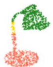
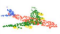
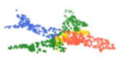
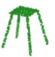
Table 3. The results of the geometric invariance verification of the proposed algorithm
|
Object |
GT |
KPConv [25] |
shift |
scaling |
PointNet++ [13] |
shift |
scaling |
|
Airplan |
|||||||
|
chair |
|||||||
|
Motorbike |
|||||||
|
Lamp |
|||||||
|
Object |
GT |
3D GCN [24] |
shift |
scaling |
My method |
shift |
scaling |
|
Airplan |
|||||||
|
chair |
|||||||
|
Motorbike |
|||||||
|
Lamp |
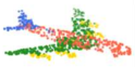
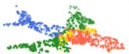
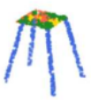
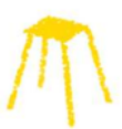
Part segmentation is visualized using ShapeNetPart. We contrast the results of our segmentation with those from PointNet++ [23] and KPConv [30]. To evaluate the invariance capabilities of each model, additional displacement (by a factor of 100) and scale (by a factor of 10) alterations are shown. Keep in mind that the designation for the ground truth element is GT.
The "Graph Convolution Algorithm Based on Visual Selectivity" is suggested in this research. The program creates a theoretical feature graph convolution algorithm based on relative amounts and presents a new graph convolutional kernel and its design process based on the visual selectivity feature. The algorithm's geometric invariance is established, and 3D point cloud processing is where it is used. Verify the performance advantages of this algorithm over the PointNet [12], PointNet++ [13], DGCNN [21], KPConv [25], and 3D-GCN [24] algorithms on the ModelNet40 and ShapeNetPart datasets. Also, confirm the algorithm's geometric invariance.
The algorithm's performance will be improved in the future in the following two ways:
(1) Algorithm parameter setting and performance optimization are realized based on the number and mode of connections between human visual cells.
(2) Examine how attention mechanisms and visual selectivity can be combined, then either enhance the existing algorithm or suggest a brand-new one.
This work is supported by the Key R & D Projects in Hebei Province of China (Grant No.: 19210111D); Science and technology planning project of Hebei Province of China (Grant No.: 15210135); The social science foundation of Hebei province of China (Grant No.: HB18TJ004 and Grant No.: HB21YS014); the Key R&D Projects in Hebei Province of China (Grant No.: 20310301D); The Higher Education Teaching Reform Research and Practice Project of Hebei Province (Grant No.: 2019GJJG510).
[1] Zhu, Y., Mottaghi, R., Kolve, E., Lim, J.J., Gupta, A., Li, F.F., Farhadi, A. (2017). Target-driven visual navigation in indoor scenes using deep reinforcement learning. In 2017 IEEE International Conference on Robotics and Automation (ICRA), 3357-3364. https://doi.org/10.1109/ICRA.2017.7989381
[2] Qi, C.R., Liu, W., Wu, C., Su, H., Guibas, L.J. (2018). Frustum pointnets for 3d object detection from RGB-d data. In Proceedings of the IEEE Conference on Computer Vision and Pattern Recognition, pp. 918-927.
[3] Luo, W., Yang, B., Urtasun, R. (2018). Fast and furious: Real time end-to-end 3d detection, tracking and motion forecasting with a single convolutional net. In Proceedings of the IEEE Conference on Computer Vision and Pattern Recognition, pp. 3569-3577.
[4] El hazzat, S., Saaidi, A., Satori, K. (2014). Multi-view passive 3D reconstruction: Comparison and evaluation of three techniques and a new method for 3D object reconstruction. In 2014 International Conference on Next Generation Networks and Services (NGNS), pp. 194-201. https://doi.org/10.1109/NGNS.2014.6990252
[5] Wu, Z., Song, S., Khosla, A., Yu, F., Zhang, L., Tang, X., Xiao, J. (2015). 3d shapenets: A deep representation for volumetric shapes. In Proceedings of the IEEE Conference on Computer Vision and Pattern Recognition, pp. 1912-1920.
[6] Szeliski, R., Lavallée, S. (1996). Matching 3-D anatomical surfaces with non-rigid deformations using octree-splines. International Journal of Computer Vision, 18(2): 171-186. https://doi.org/10.1007/BF00055001
[7] Seitz, S.M., Curless, B., Diebel, J., Scharstein, D., Szeliski, R. (2006). A comparison and evaluation of multi-view stereo reconstruction algorithms. In 2006 IEEE Computer Society Conference on Computer Vision and Pattern Recognition (CVPR'06), 1: 519-528. https://doi.org/10.1109/CVPR.2006.19
[8] Chen, X., Ma, H., Wan, J., Li, B., Xia, T. (2017). Multi-view 3d object detection network for autonomous driving. In Proceedings of the IEEE Conference on Computer Vision and Pattern Recognition, pp. 1907-1915. https://doi.org/10.48550/arXiv.1611.07759
[9] Khamsehashari, R., Schill, K. (2021). Improving deep multi-modal 3d object detection for autonomous driving. In 2021 7th International Conference on Automation, Robotics and Applications (ICARA), pp. 263-267. https://doi.org/10.1109/ICARA51699.2021.9376453
[10] Wu, Z., Song, S., Khosla, A., Yu, F., Zhang, L., Tang, X., & Xiao, J. (2015). 3d shapenets: A deep representation for volumetric shapes. In Proceedings of the IEEE Conference on Computer Vision and Pattern Recognition, pp. 1912-1920. https://doi.org/10.1109/CVPR.2015.7298801
[11] Huang, F., Wang, Z., Wu, J., Shen, Y., Chen, L. (2021). Residual triplet attention network for single-image super-resolution. Electronics, 10(17): 2072. https://doi.org/10.3390/electronics10172072
[12] Qi, C.R., Su, H., Mo, K., Guibas, L.J. (2017). Pointnet: deep learning on point sets for 3d classification and segmentation. In Proceedings of the IEEE Conference on Computer Vision and Pattern Recognition, pp. 652-660.
[13] Qi, C.R., Yi, L., Su, H., Guibas, L.J. (2017). Pointnet++: Deep hierarchical feature learning on point sets in a metric space. Advances in Neural Information Processing Systems, 30.
[14] Li, J., Pan, B., Cherkashin, E., Liu, L., Sun, Z., Zhang, M., Li, Q. (2020). 3D point cloud multi-target detection method based on PointNet++. In International Conference on Computer Engineering and Networks, 1279-1290. https://doi.org/10.1007/978-981-15-8462-6_147
[15] Chen, Y., Liu, G., Xu, Y., Pan, P., Xing, Y. (2021). PointNet++ network architecture with individual point level and global features on centroid for ALS point cloud classification. Remote Sensing, 13(3): 472. https://doi.org/10.3390/rs13030472
[16] Chai, K.Y., Stenzel, J., Jost, J. (2020). Generation, classification and segmentation of point clouds in logistic context with PointNet++ and DGCNN. In 2020 3rd International Conference on Intelligent Robotic and Control Engineering (IRCE), pp. 31-36. https://doi.org/10.1109/IRCE50905.2020.9199248
[17] Chen, Y., Xu, Y., Xing, Y., Liu, G. (2021). DGCNN network architecture with densely connected point pairs in multiscale local regions for ALS point cloud classification. IEEE Geoscience and Remote Sensing Letters, 19: 1-5. https://doi.org/10.1109/LGRS.2021.3102599
[18] Liang, Z., Yang, M., Deng, L., Wang, C., Wang, B. (2019). Hierarchical depthwise graph convolutional neural network for 3d semantic segmentation of point clouds. In 2019 International Conference on Robotics and Automation (ICRA), pp. 8152-8158. https://doi.org/10.1109/ICRA.2019.8794052
[19] Feng, M., Gilani, S.Z., Wang, Y., Zhang, L., Mian, A. (2020). Relation graph network for 3D object detection in point clouds. IEEE Transactions on Image Processing, 30: 92-107. https://doi.org/10.1109/TIP.2020.3031371
[20] Feng, M., Zhang, L., Lin, X., Gilani, S.Z., Mian, A. (2020). Point attention network for semantic segmentation of 3D point clouds. Pattern Recognition, 107: 107446. https://doi.org/10.1016/j.patcog.2020.107446
[21] Wang, Y., Sun, Y., Liu, Z., Sarma, S.E., Bronstein, M.M., Solomon, J.M. (2019). Dynamic graph CNN for learning on point clouds. ACM Transactions on Graphics (tog), 38(5): 1-12. https://doi.org/10.1145/3326362
[22] Shen, Y., Feng, C., Yang, Y., Tian, D. (2018). Mining point cloud local structures by kernel correlation and graph pooling. In Proceedings of the IEEE Conference on Computer Vision and Pattern Recognition, pp. 4548-4557. https://doi.org/10.48550/arXiv.1712.06760
[23] Liu, Y., Fan, B., Xiang, S., Pan, C. (2019). Relation-shape convolutional neural network for point cloud analysis. In Proceedings of the IEEE/CVF Conference on Computer Vision and Pattern Recognition, pp. 8895-8904. https://doi.org/10.48550/arXiv.1904.07601
[24] Lin, Z.H., Huang, S.Y., Wang, Y.C.F. (2020). Convolution in the cloud: Learning deformable kernels in 3d graph convolution networks for point cloud analysis. In Proceedings of the IEEE/CVF Conference on Computer Vision and Pattern Recognition, pp. 1800-1809.
[25] Thomas, H., Qi, C.R., Deschaud, J.E., Marcotegui, B., Goulette, F., Guibas, L.J. (2019). Kpconv: Flexible and deformable convolution for point clouds. In Proceedings of the IEEE/CVF International Conference on Computer Vision, pp. 6411-6420. https://doi.org/10.48550/arXiv.1904.08889
[26] Li, J., Chen, B.M., Lee, G.H. (2018). So-net: Self-organizing network for point cloud analysis. In Proceedings of the IEEE Conference on Computer Vision and Pattern Recognition, pp. 9397-9406.
[27] Huang, Q., Wang, W., Neumann, U. (2018). Recurrent slice networks for 3d segmentation of point clouds. In Proceedings of the IEEE Conference on Computer Vision and Pattern Recognition, pp. 2626-2635. https://doi.org/10.48550/arXiv.1802.04402
[28] Gadelha, M., Wang, R., Maji, S. (2018). Multiresolution tree networks for 3d point cloud processing. In Proceedings of the European Conference on Computer Vision (ECCV), pp. 103-118. https://doi.org/10.48550/arXiv.1807.03520
[29] Klokov, R., Lempitsky, V. (2017). Escape from cells: Deep KD-networks for the recognition of 3d point cloud models. In Proceedings of the IEEE International Conference on Computer Vision, pp. 863-872. https://doi.org/10.48550/arXiv.1704.01222
[30] Simonovsky, M., Komodakis, N. (2017). Dynamic edge-conditioned filters in convolutional neural networks on graphs. In Proceedings of the IEEE Conference on Computer Vision and Pattern Recognition, pp. 3693-3702.
[31] Yi, L., Kim, V.G., Ceylan, D., Shen, I.C., Yan, M., Su, H., Guibas, L. (2016). A scalable active framework for region annotation in 3d shape collections. ACM Transactions on Graphics (ToG), 35(6): 1-12. https://doi.org/10.1145/2980179.2980238