Harun Bingol
© 2022 IIETA. This article is published by IIETA and is licensed under the CC BY 4.0 license (http://creativecommons.org/licenses/by/4.0/).
OPEN ACCESS
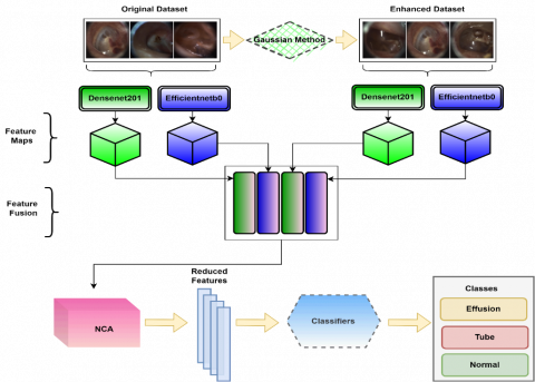
Otitis media with effusion (OME) is defined as a middle ear disease that occurs with the accumulation of fluid in the posterior part of the eardrum, usually without any symptoms. When OME disease is not treated, some negative consequences arise that deeply affect the education, social and cultural life of the patient. OME disease is a difficult issue to diagnose by specialists. In this article, autoendoscopic images of the eardrum have been classified using deep learning methods to help specialists in the diagnosis of OME. In this study, a hybrid deep model based on artificial intelligence is proposed. In the proposed hybrid model, feature maps were obtained using Efficientnetb0 and Densenet201 architectures from both the original dataset and the improved dataset using the gaussian method. Then, the merging process was applied to these feature maps. Unnecessary features are eliminated by applying NCA dimension reduction to the combined feature map. The most valuable features obtained at the end of the optimization process are classified in different machine learning classifiers. The proposed model reached a very competitive accuracy value of 98.20% in the SVM classifier.
CNN, Gaussian method, Otoendoscopic images, NCA, otitis media with effusion
OME is a serious disease that can cause hearing loss in children today [1]. OME is a disease in which acute infection is not observed, but fluid formation in the middle ear is observed [2]. Due to their nature, people feel the need to hear the sounds that emerge as a result of the events happening around them. OME causes speech disorders and hearing loss in patients. Speech impairment and hearing loss seriously affect the patient's life. For these reasons, the patient will start treatment earlier with the early diagnosis of OME. Thus, the patient will be able to integrate into social life. In addition, the patient will have a chance to receive better education. It is actually not a very correct approach to look at this situation only from the point of view of the patient. Every year, billions of dollars are spent on healthcare in the United States for the treatment of OME, and millions of boxes of antibiotics are used [3, 4]. Since this disease does not show severe symptoms, it is likely to be overlooked by experts [5]. In addition, when the disease is diagnosed, it is very important to follow up with certain periods in terms of the course of the disease. For the diagnosis of OME, otolaryngologists examine eardrum otoendoscopic images. For this disease, which is frequently observed in children and does not show any symptoms, other specialists such as pediatricians and practitioners can examine eardrum otoendoscopic images. However, these specialists are not as successful as otolaryngologists in diagnosing a disease related to the eardrum. Thus, erroneous diagnosis situations, which is an undesirable situation, may occur. Computer-aided systems should be used to prevent erroneous diagnosis situations that may arise in this way [6]. In recent years, computer-aided disease assessment applications have been widely used in the biomedical field [7-9].
1.1 Related works
Some studies in the literature using deep learning methods related to the diagnosis and classification of OME are as follows;
Wu et al., in their study, performed classification using Xception and MobilenetV2 deep architectures in the dataset they created from otoendoscopic images obtained from their own institutes and obtained accuracy values of 97.45% and 95.72%, respectively. The researchers tested the pre-trained deep models they used in the study only on their own datasets [10].
Sundgaard et al. used deep learning techniques to detect otitis media on a dataset containing 1336 otoscopy images of the tympanic membrane in their study. They stated that the accuracy rate of classifying the tympanic membrane images of the model they proposed was 85%. The researchers could compare the model they proposed in the study with the CNN architectures accepted in the literature so that the performance of the proposed model could be seen more clearly. In this way, the performance of the proposed model could be observed more clearly [11].
Crowson et al. tried to classify OME with deep learning models using a total of 338 ear images, 126 normal and 212 abnormal, taken from children for the diagnosis of OME. They used the Resnet34 architecture during the experiments. The researchers used the Resnet34 architecture in the study and obtained an accuracy value of 83.8%. Therefore, the accuracy value remained low [12].
Seneras et al. stated that they used two different deep learning architectures in the detection of eardrum abnormalities in their study. They stated that the accuracy rate they obtained was 84.4% in the first architecture, Network1, and 82.6% in the second architecture, Network2 [13].
Eroglu and Yildirim in their study, tried to classify eardrum images using deep learning techniques. During the experiments, a dataset containing 3 classes, 1 of which was normal, was used. The accuracy rate of their proposed model in classifying OME was stated as 94.27% [5].
In their study, Khan et al. stated that they performed the classification process with 95% accuracy using deep learning methods on 2484 autoendoscopic images collected by them for the diagnosis of middle ear infection and eardrum. In this study, rotation and translation processes from data augmentation methods were applied. These methods are not suitable for use as they cause memorization of the proposed model [14].
Camalan et al. used deep learning methods in the classification of OME in their study. The dataset they used during the experiments consists of normal, effusion, and tube classes containing autoendoscopic images. The dataset contains a total of 454 images. They stated that the accuracy rate they obtained in the classification of OME was 80.58%. Achieved performance criteria can be increased with new models to be developed [15].
1.2 Contribution and Novelty
In this study, it was aimed to diagnose OME by using autoendoscopic images of the eardrum. In the study, first of all, the images in the data set were improved using the Gaussian method. Then, feature maps were extracted from both the original dataset and the images in the enhanced dataset. Densenet201 and Efficientnetb0 architectures were used in feature extraction. The feature maps obtained using these two architectures are combined. In this way, different features of the same image are brought together. Therefore, the performance rates of the models have increased.
NCA dimension reduction method was applied to the feature map obtained in the last step. Since the number of features is reduced with this optimization method, the model runs faster. Finally, the optimized feature map was classified in different classifiers.
1.3 Organization of paper
In the first part of the article, general information about OME disease and its treatment is given. In the second part, detailed information about the dataset used in the study, Gaussian image enhancement method, NCA size reduction method, proposed hybrid deep model, and machine learning classifiers are given. In the third section, experimental results are given. In the fourth chapter, the experimental results are evaluated. In the fifth and last chapter, the results of the study are discussed.
The dataset used in the paper, CNN models, supervised learning methods, NCA size reduction method, Gaussian image enhancement method, and the model we proposed are explained.
2.1 Dataset description
A publicly available dataset was used during the experiments. This dataset contains a total of 454 eardrum images. There are 3 classes in total, effusion, tube, and normal in the dataset [15]. In Table 1, the number of images in each class is given. In addition, preprocessing steps were not carried out on the images in the dataset. Some tympanic images of the 3 classes in the dataset are shown in Figure 1.
Figure 1. Examples of endoscopic images in the dataset
Table 1. The number of images in each class in the dataset
|
Classes |
Effusion |
Tube |
Normal |
|
Number of images |
179 |
96 |
179 |
2.2 Deep models, Gaussian method, machine learning methods and NCA
Deep learning techniques were used to classify the eardrum images effectively. Deep models have been used frequently in recent years, especially in the fields of biomedical image processing and disease diagnosis. Thanks to deep learning, time is saved and less expert knowledge is needed. It does not need expert knowledge while performing the classification operations of deep models. In other words, unlike classical machine learning methods, feature maps are automatically generated in deep learning techniques, and manual selection is not performed. In addition, machine learning methods, unlike deep learning methods, perform data preprocessing stages. Thus, it brings the additional cost to the system in terms of hardware and takes extra time. This is another advantage of deep learning methods. In this study, the Gaussian method was applied to the original dataset in order to increase the accuracy while classifying the eardrum images. Gaussian method is a method frequently used for image enhancement in the literature. Successful results were obtained in the classification of OME images by applying the Gaussian method to the original images in the dataset. The mathematical expression of the Gaussian method is shown in Eq. (1). Thanks to the improved dataset, the features to be obtained before the classification was obtained more efficiently.
$P_G(Z)=\frac{1}{\alpha \sqrt{2 \pi}} e^{-\frac{(z-\mu)^2}{2 \sigma^2}}$ (1)
The gray level, mean value and standard deviation values are shown in Eq. (1) as Z, $\mu$, and $\sigma$, respectively. The original image with noise may have dark pixels in the bright regions and bright pixels in the dark regions. The Gaussian method can be applied to obtain the original image. Thus, the noise caused by some bit errors that may occur during the conversion of the data or during the transmission of the data with tools such as ADC (Analog Digital Converter) can be removed [16-18].
Both the original dataset and the Gauss-improved dataset were used together while extracting the feature maps of tympanic membrane images. Two different deep models were used as the base while creating the hybrid model we suggested. These models are the Efficientnetb0 and Densenet201 architectures.
The feature maps obtained from the developed hybrid method are classified by Support Vector Machines (SVM), which is one of the supervised machine learning methods [19, 20]. Furthermore, to measure the performance values of other classifiers, Decision Trees (DT) [21], k-NearestNeighbors (KNN) [22], Naive Bayes (NB) [23], Subspace Ensemble (SE) [24], and Diskriminant Analysis (DA) [25] classifiers were used. NCA method was preferred for dimension reduction in feature maps obtained with deep models. Since feature maps have been reduced in size by the NCA, processing of these features will take less time. These features will also be easier to understand. The NCA approach will remove unnecessary features.
In order to evaluate the performance metrics of the proposed hybrid model, firstly, 8 different pre-trained deep models were used to obtain results. The first of these is the Efficientnetb0 architecture. The Efficientnetb0 architecture was proposed by Tan and Le in 2019. In this proposed model, it is stated that the depth as well as the width and resolution factors affect the performance. The biggest difference of this model from other models developed before it is that for the first time, width and resolution parameters are also taken into account [26]. The other architecture, MobilenetV2, was proposed by Howard et al. in 2017. This architecture is designed for use in mobile networks with lower data processing capability [27]. The InceptionV3 architecture was developed by Szegedy et al. This model roughly consists of three parts: the initial block, the convolution block, and the classifier block. Consisting of 315 layers, this architecture takes input images in 299x299 size [28]. Alexnet architecture was developed in 2012 by Krizhevsky et al. It won the ImageNet competition held in 2012, causing deep learning to attract the attention of the scientific World [29]. Resnet50 architecture, which was developed by He et al. in 2015, became the winner of the ImageNet competition with an error rate of 3.6%. Resnet50 architecture, which has 26 million parameters, consists of 152 layers [30]. Densenet201 architecture was developed by Huang et al. in 2017. The main advantage of this architecture is that this model is denser and more efficient as it uses short links between layers. This allowed the use of small filters [31]. Googlenet, on the other hand, won the ImageNet competition held in 2014 with an error rate of 6.66%. This architecture was the first to move away from the tradition of sequentially ordering layers. In this architecture, parallel layers are used in order to reduce the memory cost and reduce the probability of memorizing the network [32]. The last used Shufflenet architecture is designed for mobile devices with limited computing power, similar to the MobilenetV2 architecture. The error rate of this architecture is stated as 7.8% [33, 34].
2.3 Proposed model
In the study, a hybrid model is proposed for the classification of OME images. In order to increase the performance of the proposed model, Gaussian image enhancement technique was applied to the OME images in the dataset. Then, separate feature maps were obtained by using 8 different deep models to create the proposed hybrid model. Then, 2 models with the highest performance ratio among these models (Efficientnetb0 and Densenet201) were used as the base in the proposed hybrid model. Using these models, feature maps were obtained from both the original dataset and the improved dataset. These resulting feature maps were then combined. In this way, different features of the same image are brought together.
NCA dimension reduction method was applied to the feature map that emerged after this step. The size of the feature map obtained after merging was 454x4000, while the size of the feature map obtained after the NCA size reduction method was 454x102. The resulting feature map was classified into 6 different machine learning classifiers. The block diagram of the proposed model is shown in Figure 2.
Figure 2. Block representation of the proposed model
When Figure 2 is examined, the "efficientnet-b0|model|head|dense|MatMul" layer of this architecture is used while obtaining the feature map using the Efficientnetb0 architecture. In Densenet201 architecture, the feature map was obtained from the "fc1000" layer.
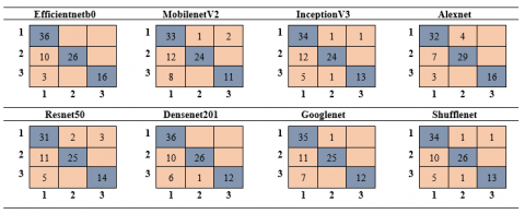
In this study, constant coefficients were used in all experiments. The results are obtained using fixed parameters in both deep learning architectures and machine learning classifiers. Again in the experiments, the cross-validation coefficient was determined as 5. The experiments were carried out on a computer with an i5 processor, 16 GB RAM, 4 GB graphics card and Windows 10 operating system. Confusion matrices were used to measure the performance of both the proposed hybrid model and other deep models. The performances of the methods were compared using the metrics Precision (Pre), Sensitivity (Sens), F-score (F1), Accuracy (Acc), Specific (Spc), False Discovery Rate (FDR), False Negative Rate (FNR), False Positive Rate (FPR). Effusion, normal, and tube classes in the confusion matrix are represented as 1, 2, and 3 respectively.
3.1 Results of pre-trained deep models
Eight different pre-trained state-of-the-art models were used in this study. It is very important to use the same parameters in all experiments in order to compare the results in the most accurate way. In this respect, we used the same parameters in the experiments. Table 2 lists the training parameters employed in these state-of-the-art models.
Table 2. Training parameters used in state-of-the-art methods
|
Environment |
Max Epochs |
Mini Batch Size |
Learn Rate |
Optimization |
|
Matlab 2021b |
5 |
8 |
1e-4 |
Sgdm |
The dataset is divided into 20% testing and 80% training. The values of the accuracy obtained from the deep architectures are listed in Table 3.
Table 3. Accuracy values of state-of-the-art models
|
Efficientnetb0 |
InceptionV3 |
MobilenetV2 |
Resnet50 |
|
85.71% |
78.02% |
74.73% |
76.92% |
|
Alexnet |
Googlenet |
Densenet201 |
Shufflenet |
|
84.62% |
79.12% |
81.32% |
80.22% |
When the confusion matrices acquired from the networks trained with state-of-the-art architectures are examined, the Efficientnetb0 is found to be the best model, with an accuracy of 85.71 percent. While the Efficientnetb0 model successfully recognized 78 of the 91 test data, it wrongly classified 13 of them.
Table 4. Confusion matrices get from state-of-the-art architectures
Table 5. Deep models + NCA + supervised learning methods
|
Deep Models / Feature Counts |
Accuracy Values obtained from the Algorithms (%) |
|||||
|
DT |
DA |
NB |
SVM |
KNN |
SE |
|
|
Efficientnetb0(39) |
79.50 |
90.50 |
88.50 |
92.50 |
89.20 |
90.10 |
|
MobilenetV2(77) |
70.70 |
88.50 |
86.60 |
89.90 |
90.50 |
90.30 |
|
InceptionV3(31) |
72.00 |
87.40 |
85.50 |
89.40 |
88.30 |
87.00 |
|
Alexnet (42) |
74.70 |
88.30 |
85.70 |
89.20 |
86.30 |
88.10 |
|
Resnet50(43) |
72.90 |
85.20 |
89.20 |
90.50 |
89.00 |
88.80 |
|
Densenet201(107) |
74.90 |
89.90 |
88.10 |
91.00 |
89.60 |
89.60 |
|
Googlenet(112) |
72.20 |
84.40 |
84.80 |
88.10 |
88.30 |
86.80 |
|
Shufflenet(147) |
73.60 |
86.10 |
85.00 |
89.40 |
87.20 |
89.60 |
Effusion was class in which the best results are obtained from the Efficientnetb0 model with an accuracy of 100 percent. All 36 Effusion images were succesfully classified by the Efficientnetb0 model. The Efficientnetb0 model succesfully classified 26 of 36 Normal images, and incorrectly classified 10 as Effusion. Finally, 16 of the 19 Tube images were correctly classified and 3 of Tube images were incorrectly classfied as Effusion by the the Efficientnetb0 model.
Furthermore, Confusion Matrices obtained using pre-trained deep architectures show that, MobilenetV2 seems the worst model with 74.73% accuracy. 68 of 91 test data were correctly classified and 23 data were incorrectly classified by MobilenetV2. MobilenetV2 model showed better performance in Effusion class. The MobilenetV2 architecture correctly classified 33 of the 36 Effusion images, , incorrectly predicted 1 as normal and 2 as tube. MobilenetV2 architecture correctly classified 24 of 36 images in Normal class and classified 12 of them as Effusion. The MobilenetV2 model successfully classified 11 of the 19 images belonging to Tube class and misclassified 8 of these images as Effusion.
It is seen in the fine-tuning tests performed on the same dataset and using fixed parameters that the classification performances of deep models may differ.
3.2 NCA, deep architecture, and feature extraction
Feature maps were obtained with pre-trained deep architectures in the second step of the study. NCA algorithm optimized the obtained feature maps and they were classified in traditional supervised learning methods. Default values for the parameters are utilized for feature selection in the NCA algorithm. For estimating the feature weights, Stochastic Gradient Descent (SGD) was chosen as the solvent. The value of the Verbosity Level Indicator (Verbose) is chosen as 1 for rapid results. The size of the feature maps get using state-of-the-arts models is 454x1000 in each model. When the NCA algorithm is separately performed to the extracted features, the obtained new feature map size is 454x39 in Efficientnetb0, 454x77 in MobilenetV2, 454x31 in InceptionV3, 454x42 in Alexnet, 454x43 in Resnet50, 454x107 in Densenet201, 454x112 in Googlenet and 454x147 in Shufflenet. Table 5 lists the accuracy values obtained from deep models.
The highest values for the accuracy metric were achieved by the Densenet201 and Efficientnetb0 architectures, as demonstrated in Table 5. Thus, these two architectural models are utilized in the proposed methodology. Confusion matrices obtained from two architectures are listed in Table 6.
Table 6. Confusion matrices
In addition, Table 5 shows that Densenet201 reached the second-highest accuracy rate with 91%. When Table 6 is examined, Densenet201 architecture correctly classified 166 of 179 Effusion images, while it misclassified 12 as Normal class and 1 as Tube class. Again, while this architecture correctly classified 158 of 179 Normal class images, 21 of them were incorrectly classified as Effusion class. While the Densenet201 architecture correctly classified 89 of the 96 Tube class images, 7 of them were incorrectly classified as Effusion class.
3.3 Proposed model
Feature maps were obtained using Densenet201 and Efficientnetb0 architectures from both the original dataset and the dataset, which was improved using the Gaussian method. Then, these features were combined and a feature map was obtained. The size of the feature map formed after merging was 454x4000. For eliminating the worthless features from the feature map, NCA algorithm was utilized. Default parameter values were used for the NCA algorithm. SGD was chosen as the solvent and value for Verbose was selected as 1. The new feature map size formed after the optimization is 454x102. Table 7 lists the accuracy values obtained from traditional supervised learning algorithms in the proposed model.
The features extracted from the proposed hybrid model are classified by different supervised intelligent classifaction methods. SVM (Quadratic Version) achieved the best results with an accuracy value of 98.20%. DTs seems the worst algorithm with an accuracy value with 83.90% for this task. SVM, SE, and DA seem the most successfull classifiers methods. Table 8 lists the confusion matrices obtained from the used supervised learning methods.
SVM, SE, and DA algorithms seem the best succesfull methods with the highest accuracy rates obtained from the proposed model. For example, SVM method succescfully classified 446 of 454 otoendoscopic images of the eardrum while insuccesfully classified the rest. Performance metrics of the proposed model are listed in Table 9.
When the obtained values for the performance metrics data are checked, it seems that the only accuracy value is not an appropirate for performance comparison. While the highest Sensitivity value with 100% was obtained in the Tube class, the highest accuracy value with 98.32% was obtained in the Effusion class and Normal class by the proposed model. Thus, the proposed model in this study achieved the best success for diagnosing otoendoscopic images of the eardrum. Therefore, it is thought that the proposed model can be used in the diagnosis of tympanic otoendoscopic images.
Eight deep network architectures and six intelligent supervised classifiers were used for classification of the tympanic otoendoscopic images. The model proposed in this study seems to achieve the highest values for the accuracy. Values for the accuracy metric obtained from deep neural architecture and intelligent supervised learning methods are listed in Table 10.
Table 7. Accuracy values obtained from the proposed model
|
|
Accuracy Values Obtained from the Algorithms (%) |
|||||
|
DT |
DA |
NB |
SVM |
KNN |
SE |
|
|
Proposed Model |
83.90 |
97.80 |
97.60 |
98.20 |
97.40 |
98.00 |
Table 8. Confusion matrices obtained from the proposed model
Table 9. Performance metric values of the proposed model
|
|
Acc.(%) |
Spc.(%) |
Sens.(%) |
Pre.(%) |
FPR(%) |
F1(%) |
FNR(%) |
FDR(%) |
|
Effusion |
98.32 |
98.90 |
97.23 |
98.32 |
1.09 |
97.77 |
2.76 |
1.67 |
|
Normal |
98.32 |
98.90 |
98.32 |
98.32 |
1.09 |
98.32 |
1.67 |
1.67 |
|
Tube |
97.92 |
99.44 |
100.00 |
97.91 |
0.55 |
98.94 |
0.00 |
2.08 |
Table 10. Values of the performance metrics obtained from the deep architectures
|
|
Softmax(%) |
DA(%) |
DT(%) |
KNN(%) |
NB(%) |
SVM(%) |
SE(%) |
|
Efficientnetb0 |
85.71 |
90.50 |
79.50 |
89.20 |
88.50 |
92.50 |
90.10 |
|
MobilenetV2 |
74.73 |
88.50 |
70.70 |
90.50 |
86.60 |
89.90 |
90.30 |
|
InceptionV3 |
78.02 |
87.40 |
72.00 |
88.30 |
85.50 |
89.40 |
87.00 |
|
Alexnet |
84.62 |
88.30 |
74.70 |
86.30 |
85.70 |
89.20 |
88.10 |
|
Resnet50 |
76.92 |
85.20 |
72.90 |
89.00 |
89.20 |
90.50 |
88.80 |
|
Densenet201 |
81.32 |
89.90 |
74.90 |
89.60 |
88.10 |
91.00 |
89.60 |
|
Googlenet |
79.12 |
84.40 |
72.20 |
88.30 |
84.80 |
88.10 |
86.80 |
|
Shufflenet |
80.22 |
86.10 |
73.60 |
87.20 |
85.00 |
89.40 |
89.60 |
|
Proposed Model |
- |
97.80 |
83.90 |
97.40 |
97.60 |
98.20 |
98.00 |
Table 11. Studies on classification of eardrum images
|
Reference |
Method |
Number of Images |
Number of Class |
Acc(%) |
|
Wu et al. [10] |
Xception |
12203 |
3 |
97.45 |
|
|
MobilenetV2 |
12203 |
3 |
95.72 |
|
Sundgaard et al. [11] |
InceptionV3 |
1336 |
3 |
85.00 |
|
Crowson et al. [12] |
Resnet34 |
338 |
2 |
83.80 |
|
Seneras et al. [13] |
InceptionV3 |
409 |
2 |
84.40 |
|
Eroglu and Yildirim [5] |
(Efficientnetb0 + Darknet53 + Densenet201) + NCA + SVM |
454 |
3 |
94.27 |
|
Khan et al. [14] |
Grad-CAM+Densenet161 |
2484 |
3 |
95.00 |
|
Camalan et al. [15] |
Inception-Resnet-V2 |
454 |
3 |
80.58 |
|
Proposed Model |
(Efficientnetb0 + Densenet201) + Gaussian Method + NCA + SVM |
454 |
3 |
98.20 |
Acute Otitis Media (AOM) is defined as a fluid collection in the middle ear, in other words, mucositis [35, 36]. It has been reported that effusions lasting more than 4 months are seen in 1/3 of children with AOM. Thus, the Otitis Media with Effusion (OME) situation arises [37]. OME is usually seen in children aged 7 months to 6 years without any signs of acute infection [38]. OME can cause deafness in children if left untreated. Long-term deafness in children also brings speech disorders. In some cases, OME can cause pain due to pressure in the middle ear of the patient [39]. Since this disease does not show serious symptoms, it can sometimes be overlooked by specialists. Surgical methods are generally used in the treatment of OME. The fluid collected in the middle ear is drained by applying myringotomy to the eardrum, that is, by opening a small hole. Since this hole opened in the eardrum will close very early, a tympanostomy tube is placed in this hole. The main task of the tube is to ventilate the middle ear cavity by preventing the opening of the hole from closing. Another benefit of tympanostomy tube insertion in OME cases is to contribute to the development of mastoid cells. It has also been demonstrated by some studies that mastoid cell size is effective on OME prognosis [40-42]. Early diagnosis of OME is extremely important. When otolaryngologists examine otoendoscopic images, they can diagnose approximately 70% correctly. In addition, pediatricians can make an accurate diagnosis of approximately 50%. General practitioners can diagnose OME with approximately 45% accuracy [5].
Deep learning methods have been widely used in the classification of disease images in the biomedical field, especially in the last 10 years [43, 44]. Classification of tympanic autoendoscopic images is not always easy. Dirty middle ear or thick eardrum complicates the classification process. It is known that computer-aided systems are extremely beneficial to overcome all these negativities.
When Table 11 is examined, an accuracy value of 98.20% was obtained in the hybrid model we proposed. It will be seen that this accuracy value is a very competitive value when compared with the literature. The results of the experiments show that the hybrid deep model we have proposed can be used in the classification of otoendoscopic images of the eardrum.
The main benefit of this study is the detection of OME with the help of computer-aided systems in rural areas where there are not enough otolaryngologists. Thanks to the proposed hybrid model, the workload of otolaryngologists and other medical professionals will be alleviated. In this way, otolaryngologists will be able to serve more patients. Thanks to the proposed hybrid model, the probability of success of the treatment process will increase since patients will be diagnosed earlier.
There are some limitations of this study. The most important of these is that the number of images in the dataset is not enough. In our future studies, it is among our aims to include more experts on OME in the study team and to work with eardrum images of more patients from different regions.
Because OME is a prevalent disease that can lead to serious problems if left untreated, it’s critical to get it diagnosed and treated as soon as possible. In addition, during the patient’s follow-up, the eardrum and tube should be examined. The variations in interpretation between doctors will be avoided with the model we have provided for the diagnosis and follow-up of endoscopic pictures of the eardrum, and the patient’s treatment process will begin sooner.
We thank the researchers who shared the dataset.
[1] Davidson, J., Hyde, M.L., Alberti, P.W. (1989). Epidemiologic patterns in childhood hearing loss: A review. International Journal of Pediatric Otorhinolaryngology, 17(3): 239-266. https://doi.org/10.1016/0165-5876(89)90051-7
[2] Rosenfeld, R.M., Shin, J.J., Schwartz, S.R., Coggins, R., Gagnon, L., Hackell, J.M., Hoelting, D., Hunter, L.L., Kummer, A.W., Payne, S.C., Poe, D.S., Veling, M., Vila, P.M., Walsh, S.A., Corrigan, M.D. (2016). Clinical practice guideline: Otitis media with effusion (update). Otolaryngology–Head and Neck Surgery, 154(1_suppl): S1-S41. https://doi.org/10.1177/0194599815623467
[3] Altıntaş, M., Muluk, N.B., Peng, K.A. (2021). What is the significance of rhinitis in otitis media with effusion? Challenges in Rhinology, 159-168. https://doi.org/10.1007/978-3-030-50899-9_18
[4] Samuels, T.L., Khampang, P., Espahbodi, M., McCormick, C.A., Chun, R.H., McCormick, M.E., Yan, K., Kerschner, J.E., Johnston, N. (2022). Association of pepsin with inflammatory signaling and effusion viscosity in pediatric otitis media. The Laryngoscope, 132(2): 470-477. https://doi.org/10.1002/lary.29749
[5] Eroğlu, O., Yildirim, M. (2021). Automatic detection of eardrum otoendoscopic images in patients with otitis media using hybrid‐based deep models. International Journal of Imaging Systems and Technology, 32(3): 717-727. https://doi.org/10.1002/ima.22683
[6] Cengil, E., Çınar, A., Yıldırım, M. (2022). A hybrid approach for efficient multi‐classification of white blood cells based on transfer learning techniques and traditional machine learning methods. Concurrency and Computation: Practice and Experience, 34(6): e6756. https://doi.org/10.1002/cpe.6756
[7] Eroğlu, Y., Yildirim, M., Çinar, A. (2021). Convolutional Neural Networks based classification of breast ultrasonography images by hybrid method with respect to benign, malignant, and normal using mRMR. Computers in Biology and Medicine, 133: 104407. https://doi.org/10.1016/j.compbiomed.2021.104407
[8] Eroğlu, O., Eroğlu, Y., Yıldırım, M., Karlıdag, T., Çınar, A., Akyiğit, A., Kaygusuz, İ., Yıldırım, H., Keleş, E., Yalçın, Ş. (2022). Is it useful to use computerized tomography image-based artificial intelligence modelling in the differential diagnosis of chronic otitis media with and without cholesteatoma? American Journal of Otolaryngology, 43(3): 103395. https://doi.org/10.1016/j.amjoto.2022.103395
[9] Yaman, O., Tuncer, T. (2022). Exemplar pyramid deep feature extraction based cervical cancer image classification model using pap-smear images. Biomedical Signal Processing and Control, 73: 103428. https://doi.org/10.1016/j.bspc.2021.103428
[10] Wu, Z., Li, Z.Q., Li, L., Pan, H.G., Chen, G.W., Fu, Y.P., Qiu, Q.H. (2021). Deep learning for classification of pediatric otitis media. The Laryngoscope, 131(7): E2344-E2351. https://doi.org/10.1002/lary.29302
[11] Sundgaard, J.V., Harte, J., Bray, P., Laugesen, S., Kamide, Y., Tanaka, C., Paulsen, R.R., Christensen, A.N. (2021). Deep metric learning for otitis media classification. Medical Image Analysis, 71: 102034. https://doi.org/10.1016/j.media.2021.102034
[12] Crowson, M.G., Hartnick, C.J., Diercks, G.R., Gallagher, T.Q., Fracchia, M.S., Setlur, J., Cohen, M.S. (2021). Machine learning for accurate intraoperative pediatric middle ear effusion diagnosis. Pediatrics, 147(4): e2020034546. https://doi.org/10.1542/peds.2020-034546
[13] Senaras, C., Moberly, A.C., Teknos, T., Essig, G., Elmaraghy, C., Taj-Schaal, N., Yua, L., Gurcan, M.N. (2018). Detection of eardrum abnormalities using ensemble deep learning approaches. Medical Imaging 2018: Computer-Aided Diagnosis. 2018. International Society for Optics and Photonics. https://doi.org/10.1117/12.2293297
[14] Khan, M.A., Kwon, S., Choo, J., Hong, S.M., Kang S.H., Park, I., Kim, S.K., Hong, S.J. (2020). Automatic detection of tympanic membrane and middle ear infection from Oto-endoscopic images via convolutional neural networks. Neural Networks, 126: 384-394. https://doi.org/10.1016/j.neunet.2020.03.023
[15] Camalan, S., Niazi, M.K.K., Moberly, A.C., Teknos, T., Essig, G., Elmaraghy, C., Taj-Schaal, N., Gurcan, M.N. (2020). OtoMatch: Content-based eardrum image retrieval using deep learning. Plos One, 15(5): e0232776. https://doi.org/10.1371/journal.pone.0232776
[16] Loh, Y.P., Liang, X., Chan, C.S. (2019). Low-light image enhancement using Gaussian Process for features retrieval. Signal Processing: Image Communication, 74: 175-190. https://doi.org/10.1016/j.image.2019.02.001
[17] Ma, J., Fan, X., Ni, J., Zhu, X., Xiong, C. (2017). Multi-scale retinex with color restoration image enhancement based on Gaussian filtering and guided filtering. International Journal of Modern Physics B, 31(16-19): 1744077. https://doi.org/10.1142/S0217979217440775
[18] Hanumantharaju, M., Ravishankar, M., Rameshbabu, D. (2013). Design of novel algorithm and architecture for Gaussian based color image enhancement system for real time applications. In: Unnikrishnan, S., Surve, S., Bhoir, D. (eds) Advances in Computing, Communication, and Control. ICAC3 2013. Communications in Computer and Information Science, vol 361. Springer, Berlin, Heidelberg. https://doi.org/10.1007/978-3-642-36321-4_56
[19] Suykens, J.A.K., Vandewalle, J. (1999). Least squares support vector machine classifiers. Neural Processing Letters, 9(3): 293-300. https://doi.org/10.1023/A:1018628609742
[20] Özyurt, F., Sert, E., Avci, D. (2022). Ensemble residual network features and cubic-SVM based tomato leaves disease classification system. Traitement du Signal, 39(1): 71-77. https://doi.org/10.18280/ts.390107
[21] Safavian, S.R., Landgrebe, D. (1991). A survey of decision tree classifier methodology. IEEE Transactions on Systems, Man, and Cybernetics, 21(3): 660-674. https://doi.org/10.1109/21.97458
[22] Keller, J.M., Gray, M.R., Givens, J.A. (1985). A fuzzy k-nearest neighbor algorithm. IEEE Transactions on Systems, man, and Cybernetics, SMC-15(4): 580-585. https://doi.org/10.1109/TSMC.1985.6313426
[23] Rish, I. (2001). An empirical study of the naive Bayes classifier. IJCAI 2001 Workshop on Empirical Methods in Artificial Intelligence.
[24] Kodovsky, J., Fridrich, J., Holub, V. (2011). Ensemble classifiers for steganalysis of digital media. IEEE Transactions on Information Forensics and Security, 7(2): 432-444. https://doi.org/10.1109/TIFS.2011.2175919
[25] Alkan, A., Günay, M. (2012). Identification of EMG signals using discriminant analysis and SVM classifier. Expert Systems with Applications, 39(1): 44-47. ttps://doi.org/10.1016/j.eswa.2011.06.043
[26] Tan, M., Le, Q. (2019). Efficientnet: Rethinking model scaling for convolutional neural networks. International Conference on Machine Learning. PMLR.
[27] Howard, A.G., Zhu, M., Chen, B., Kalenichenko, D., Wang, W., Weyand, T., Andreetto, M., Adam, H. (2017). Mobilenets: Efficient convolutional neural networks for mobile vision applications. arXiv preprint arXiv:1704.04861.
[28] Szegedy, C., Ioffe, S., Vanhoucke, V., Alemi, A. (2017). Inception-v4, inception-ResNet and the impact of residual connections on learning. Thirty-first AAAI Conference on Artificial Intelligence, pp. 4278-4284.
[29] Krizhevsky, A., Sutskever, I., Hinton, G.E. (2012). ImageNet classification with deep convolutional neural networks. Communications of the ACM, 60(6): 84-90. https://doi.org/10.1145/3065386
[30] He, K., Zhang, X., Ren, S., Sun, J. (2016). Deep residual learning for image recognition. 2016 IEEE Conference on Computer Vision and Pattern Recognition (CVPR), pp. 770-778. https://doi.org/10.1109/CVPR.2016.90
[31] Huang, G., Liu, Z., Van Der Maaten, L., Weinberger, K.Q. (2017). Densely connected convolutional networks. 2017 IEEE Conference on Computer Vision and Pattern Recognition (CVPR), pp. 2261-2269. https://doi.org/10.1109/CVPR.2017.243
[32] Szegedy, C., Liu, W., Jia, Y., Sermanet, P., Reed, S., Anguelov, D., Erhan, D., Vanhoucke, V., Rabinovich, A. (2015). Going deeper with convolutions. 2015 IEEE Conference on Computer Vision and Pattern Recognition (CVPR), pp. 1-9. https://doi.org/10.1109/CVPR.2015.7298594
[33] Zhang, X., Zhou, X., Lin, M., Sun, J. (2018). ShuffleNet: An extremely efficient convolutional neural network for mobile devices. 2018 IEEE/CVF Conference on Computer Vision and Pattern Recognition, pp. 6848-6856. https://doi.org/10.1109/CVPR.2018.00716
[34] Özyurt, F. (2021). Automatic detection of COVID-19 disease by using transfer learning of light weight deep learning model. Traitement du Signal, 38(1): 147-153. https://doi.org/10.18280/ts.380115
[35] Teele, D.W., Rosner, J.O.K. (1989). Epidemiology of otitis media during the first seven years of life in children in greater Boston: A prospective, cohort study. Journal of Infectious Diseases, 160(1): 83-94. https://doi.org/10.1093/infdis/160.1.83
[36] Damoiseaux, R.A., Rovers, M.M., Van Balen, F.A.M., Hoes, A.W., de Melker, R.A. (2006). Long-term prognosis of acute otitis media in infancy: Determinants of recurrent acute otitis media and persistent middle ear effusion. Family Practice, 23(1): 40-45. https://doi.org/10.1093/fampra/cmi083
[37] Morris, P.S., Leach, A.J., Silberberg, P., Mellon, G., Wilson, C., Hamilton, E., Beissbarth, J. (2005). Otitis media in young Aboriginal children from remote communities in Northern and Central Australia: A cross-sectional survey. BMC Pediatrics, 5(1): 1-10. https://doi.org/10.1186/1471-2431-5-27
[38] Chonmaitree, T., Revai, K., Grady, J.J., Clos, A., Patel, J.K., Nair, S., Fan, J., Henrickson, K.J. (2008). Viral upper respiratory tract infection and otitis media complication in young children. Clinical Infectious Diseases, 46(6): 815-823. https://doi.org/10.1086/528685
[39] Griffin, G., Flynn, C.A. (2011). Antihistamines and/or decongestants for otitis media with effusion (OME) in children. Cochrane Database of Systematic Reviews, 2011(9): CD003423. https://doi.org/10.1002/14651858.CD003423.pub3
[40] Prymula, R., Peeters, P., Chrobok, V., Kriz, P., Novakova, E., Kaliskova, E., Kohl, I., Lommel, P., Poolman, J., Prieels, J., Schuerman, L. (2006). Pneumococcal capsular polysaccharides conjugated to protein D for prevention of acute otitis media caused by both Streptococcus pneumoniae and non-typable Haemophilus influenzae: A randomised double-blind efficacy study. The Lancet, 367(9512): 740-748. https://doi.org/10.1016/S0140-6736(06)68304-9
[41] Kaleida, P.H., Casselbrant, M.L., Rockette, H.E., Paradise, J.L., Bluestone, C.D., Blatter, M.M., Reisinger, K.S., Wald, E.R., Supance, J.S. (1991). Amoxicillin or myringotomy or both for acute otitis media: Results of a randomized clinical trial. Pediatrics, 87(4): 466-474.
[42] Paradise, J.L. (1980). Otitis media in infants and children. Pediatrics, 65(5): 917-943. https://doi.org/10.1542/peds.65.5.917
[43] Çınar, A., Yıldırım, M., Eroğlu, Y. (2021). Classification of pneumonia cell images using improved ResNet50 model. Traitement du Signal, 38(1): 165-173. https://doi.org/10.18280/ts.380117
[44] Bulla, P., Anantha, L., Peram, S. (2020). Deep neural networks with transfer learning model for brain tumors classification. Traitement du Signal, 37(4): 593-601. https://doi.org/10.18280/ts.370407