Luo Qiu | Qiuhua He | Deqing Yu* | Junde Xie
© 2022 IIETA. This article is published by IIETA and is licensed under the CC BY 4.0 license (http://creativecommons.org/licenses/by/4.0/).
OPEN ACCESS
High resolution images can better reflect the size, shape and structural characteristics of ground objects, but due to factors such as purchase cost and observation period, it is often difficult to meet the practical application needs. Sub-pixel mapping technology can effectively improve the resolution of the results, which solves the above problem to some extent. The relevant algorithms of sub-pixel mapping include mixed pixel decomposition, end pixel extraction, sub-pixel positioning and other sub fields. The most classical sub-pixel positioning methods often use spatial correlation to define the positioning criteria. In this paper, NDWI and OTSU segmentation are used to constrain sub-pixel decomposition to some extent, which improves the performance of PSA algorithm, so as to more accurately extract river shoreline information, improve the resolution of monitoring on shoreline erosion collapse and dynamic change in the bank collapse area, and enhance the applicability of satellite remote sensing in the bank collapse monitoring field.
remote sensing image, sub-pixel positioning, bank collapse, monitoring
Bank collapse is a kind of geological disaster [1] in which the river bank collapses and landslide occurs when the riverbank is simultaneously affected by water erosion and riverbed boundary conditions. Bank collapse brings hidden danger to flood control work, and at the same time causes land loss and difficulties in project construction and maintenance. It is now a hot issue in water conservancy [2]. Therefore, it is of great significance to study the means and methods of effective monitoring on bank collapse.
At present, the research on bank collapse monitoring involves a variety of tools and platforms, including manual inspection, unmanned survey ship, unmanned aerial vehicle, radar, satellite remote sensing, etc. Among them, satellite remote sensing can monitor the bank collapse area in large scale and high frequency, with high application value and potential. Zhou [3] analyzed the collapse of Chaohu Lake shore using remote sensing images. Yang et al. [4] used aerial photos, TM and ETM images to investigate the shore-strap changes of the Yangtze River in Anhui section and the bank collapse thereof. Yao et al. [5] studied the bank collapse situation from 1958 to 2008 using remote sensing data.
Although high-resolution images can better reflect the size, shape and structural characteristics of the ground objects, they are often difficult to meet the demand for observation of bank collapse areas due to such factors as purchase cost and observation period. The sub pixel mapping technology can effectively improve the resolution of the results, which solves the above problem to some extent. The related algorithms of sub-pixel mapping include mixed pixel decomposition, end pixel extraction, sub-pixel location and other sub fields. The most classical sub-pixel positioning methods often use spatial correlation to define the positioning criteria. Mertens et al. [6] use the spatial attraction model to carry out sub-pixel positioning. Each sub-pixel is attracted by different land types in space, and the maximum attraction category is taken as the land type of the sub-pixel. Atkinson et al. put forward the pixel exchange method [7], which first generates a random sub-pixel matrix and then obtains the final positioning result through continuous exchange. With the development of machine learning, many sub-pixel localization methods have been developed. Tatem et al. [8] use Hopfield neural network to conduct sub-pixel positioning. Chen et al. [9] proposed a sub-pixel localization method for offset images combining with BP neural network, effectively solving the problems of inconsistency between the relevant assumptions of spatial relations and reality, as well as the saw-tooth effect. Arun et al. [10] used CNN network and LineNet network for soft classification during sub-pixel positioning. He et al. [11] proposed a convolutional neural network framework for sub-pixel location. Song et al. [12] proposed a new SSM framework for hyper-spectral images, using the theory of multi-objective optimization to solve the sub-pixel positioning problem.
For the monitoring of bank collapse, this paper abstracts it as a generalized problem of water extraction, and further evaluates the specific situation of bank collapse by extracting the shoreline. In the research field related to water body and shoreline extraction, Zhang et al. [13] conducted sub-pixel mapping experiment using MYD09G daily surface reflectance data, which can effectively extract the water body in the Dongting Lake area. He [14] used spatial mapping table to locate sub-pixels of water bodies. Chang et al. [15] used DEM to obtain river network classification data, which are taken as a supplement for input to obtain a flood inundation map with higher accuracy. Hong et al. [16] proposed an automatic sub-pixel coastline extraction method based on hyper-spectral satellites.
At present, there are few researches on the sub-pixel algorithms that are applied to bank collapse. In this paper, aiming at the problem of insufficient resolution of commonly used satellite remote sensing, mixed pixel decomposition and sub-pixel positioning technology are used to more accurately extract river shoreline information, improve the monitoring resolution, and enhance the applicability of satellite remote sensing in the field of bank collapse monitoring.
2.1 Linear mixed pixel decomposition
In the linear mixed pixel decomposition method, the spectrum of mixed pixels is formed by the linear combination of various pure ground objects and are calculated considering the practical significance and additional conditions [17, 18].
The reflectivity of the mixed pixel is equal to the weighted sum of reflectivity between the end cells, and the mathematical expression is:
$f_k=\sum_{i=1}^n p_i \times r_{i, k}+\varepsilon_k$ (1)
In the above formula, n represents the number of ground object types, pi,k refers to the abundance value of the ith class of ground object, ri,k refers to the reflectivity of the ith ground object in the kth waveband, fk is the mixed pixel reflectance of the kth waveband and εk is the error term. In the form of matrix, it can be expressed as:
$F=P R+\varepsilon$ (2)
F is the vector composed by the reflectivity of the mixed pixel on each band, α is the abundance vector, and R is the end element reflectivity vector, and ε is the residual. This is the basic expression of linear mixed pixel decomposition.
It is supposed that there are m equations in total, and the solution objective is:
$\min \sum_{k=1}^m\left(f_k-\sum_{i=1}^n p_i \times r_{i, k}\right)^2$ (3)
Considering the actual situation of remote sensing images, two additional constraints must be added, namely, the sum of the weights of the end elements must be 1, and the range of abundance of each land category must be between 0-1, which is expressed by the formula:
$\left\{\begin{array}{l}\sum_{i=1}^n p_i=1 \\ 0 \leq p_i \leq 1\end{array}\right.$ (4)
By using the above three formulas and the fully constrained least square law to solve, the abundance value of various ground objects in each pixel can be achieved.
2.2 Sub-pixel positioning
In this paper, pixel exchange method is used to locate sub-pixels. In the traditional pixel exchange method, the algorithm results are very sensitive to the accuracy of abundance calculation, and the error caused by the abundance results will cause a lot of noise in the location results. In this paper, before adopting sub-pixel location algorithm, NDWI index is added to filter and screen, and all pixels are divided into two parts for processing. Potential pixels are screened by this index, and then sub-pixel location is carried out using exchange method to minimize the dependence of the algorithm on abundance accuracy.
2.2.1 Water pixel pretreatment
In this paper, NDWI is used for preliminary processing of potential pixels. The normalized difference water index (NDWI) is designed to extract water body ranges. The normalization based on the characteristics of water bodies in green waveband and near-infrared band can effectively distinguish water bodies from non-water bodies. The calculation expression is:
$N D W I=\frac{R_g-R_{n i r}}{R_g+R_{n i r}}$ (5)
where, Rg and Rnir are the reflectance of green band and near infrared band respectively.
All water body pixels are divided into two parts for confirmation. For the pixels to be decomposed that meet the requirements of similar non-central pixels in the sliding window, they are divided into boundary pixels for further decomposition, while other pixels retain their original attributes.
The maximum inter class variance (OTSU algorithm) is used to determine the pixel attributes. OTSU was proposed by Japanese scholar Otsu [19]. This method has good adaptability and can easily and quickly calculate the segmentation threshold. The target image is divided into Class A and Class B. First, the inter class variance is defined as:
$\sigma^2=P_a(\operatorname{mean}(A)-M)^2+P_b(\operatorname{mean}(B)-M)^2$ (6)
Among them, mean represents the average value of this category, P represents the probability of belonging to this category, and M represents the average value of the whole image. The ultimate goal of OTSU algorithm is to find a maximum threshold T, which makes σ2 the maximum.
2.2.2 Pixel exchange method
In order to determine the specific location of ground objects, this paper uses the pixel exchange method to carry out sub-pixel positioning. The pixel exchange method was proposed by Atkinson. Its basic principle is to calculate based on the direct space gravity between each sub-pixel and the domain sub-pixel within a certain window size around. In this paper, only water and non-water land types are considered, that is, the specific steps for sub-pixel positioning of each mixed pixel are as follows:
(1) The number of sub-pixels of target objects and the number of sub-pixels of non- target objects are calculated according to the abundance of target objects of mixed pixels. The sub-pixel matrix in the mixed pixel is initialized. In this way, a random s×s sub-pixel matrix is obtained, with 1 representing the target land class and 0 representing the non-target land class. S is the multiple of decomposition.
(2) The space gravity of each sub-pixel is calculated. The pixel number currently calculated is set as k, and the formula for calculating the spatial gravity between the central pixel and the sub-pixel in its neighborhood is as follows:
$S_k=\sum_{i=1}^m \lambda_{k i} C_i$ (7)
Ci is calculated using the following formula:
$C_i=\left\{\begin{array}{l}1, \text { Adjacent pixels belong to the target category} \\ 0, \text { Adjacent pixels do not belong to the target category} \end{array}\right.$ (8)
λij is the weight related to distance, and the calculation formula is:
$\lambda_{i j}=\exp \left(\frac{-d_{i j}}{\alpha}\right)$ (9)
-dij is the Euclidean distance between central pixel i and adjacent pixel j, and α is an exponential parameter, which can be adjusted according to the application.
(1) Pixel exchange. After obtaining the spatial gravity of each sub-pixel in the mixed pixel, the sub-pixel A with the lowest spatial gravity in the target land category and the sub-pixel B with the highest spatial gravity in the non-target land category can be found. We can compare the size of their spatial gravity. If the spatial gravity of A is smaller than that of B, change the code of A to 0 and the code of B to 1, thus completing the exchange.
(2) During the iterative traversal of the whole image, the above process is repeated.
3.1 Study area
Jingjiang River section is from Zhicheng in Hubei Province to Chenglingji in Yueyang County, Hunan Province, in the Yangtze River basin, with a total length of about 360km, and the river course is winding. Large scale bank collapse in this reach has been basically controlled at present, but there are still some small scale of bank collapse.
The study area of this paper is Jianli Bend of Jingjiang River and Dengpanzhou Bend of Songzi River. The longitude range of Jianli Bend is within the range of 112.87°-112.95°, and the latitude range is about 29.73°-28.82°. The longitude of Dengpanzhou Bend is about 111.73°-1121.79°, and the latitude range is about 30.34°-30.39°.
3.2 Data source and preprocessing
The data uses the remote sensing image of Sentinel-2 downloaded by USGS on the same day as the verification data. Sentinel 2 has undergone atmospheric correction and other pre-processing. In this paper, four bands with a resolution of 10 meters are used, including three visible light bands and one near-infrared band. The downloaded data shall go through atmospheric correction and accurate registeration with the verification image of the corresponding date.
The verification data in experimental area I use High-resolution No. 2 data, which has been preprocessed through radiometric calibration, atmospheric correction, ortho correction, fusion, etc., and the original resolution is 1 meter. The validation data in experimental area II uses UAV aerial data with a resolution of 0.25m. For details, see Table 1.
Table 1. Experiment data
|
Experiment area |
Image decomposition |
Image date |
Reference image |
Image date |
|
Jianli Bend |
Sentinel-2 |
Dec.6, 2016 |
High-resolution No. 2 image |
Dec.6, 2016 |
|
Dengpanzhou Bend |
Sentinel-2 |
Oct.10, 2018 |
UAV image |
Oct.9, 2018 |
3.3 Experimental results and analysis
Considering the scope of bank collapse and the surrounding actual situation in the study area, this paper covers vegetation, bare soil and three types of end elements. In the Sentinel 2 image of the current period, pure pixels of various kinds of ground objects are manually extracted. If necessary, UAV images and high resolution images of the previous period can be used as prior data to obtain the corresponding spectral curves of the three types of ground objects.
The experimental results were compared with the original resolution water extraction results, the results obtained through the traditional pixel exchange method, and the extraction method in this paper. Clustering de-noising is performed on the experimental results figures, and the operator size is 3×3, to eliminate the noise in the image. The sub-pixel decomposition scale is all 4, that is, the resolution of the decomposed result is changed from 10 meters to 2.5 meters, and the reference image is resampled to 2.5 meters to keep the resolution of the sub-pixel decomposition results consistent. The research mainly uses five methods: water body extraction based on the original image, the water body extraction based on sentinel 2, SPSAM, PSA, NPSA (NDWI+PSA). Because the reference image is Unmanned Aerial Vehicles imagery in Dengpanzhou area, object -oriented method to extract water bodies is better. And random forest algorithms are adopted in the Jianli Area.
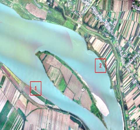
Figure 1 is the schematic diagram of the bank collapse area at the bend of Dengpanzhou, where two bank collapse areas are marked and mainly studied. The following shows the binary image of the results extracted with five methods, in which the black part is non-water body, and the gray part is the extracted water body.
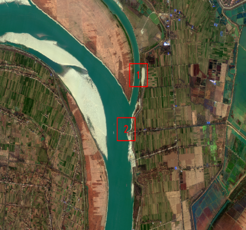
Figure 4 is the diagram of the bank collapse area of Jianli Bend, and two spots in the bank collapse area are studied.
Figure 1. Bank collapse area at the bend of Dengpanzhou (Oct.10, 2018)
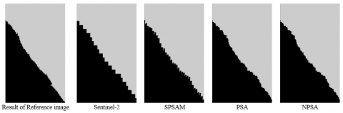
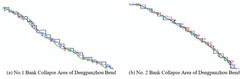
Figure 2. Contrast of enlarged local area of Dengpanzhou No. 1 Bank Collapse Area
Figure 3. Contrast of enlarged local area of Dengpanzhou No. 2 Bank Collapse Area
Figure 4. Sketch map of the bank collapse area in Jianli Bend (Dec. 9, 2016)
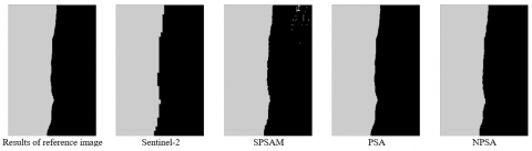
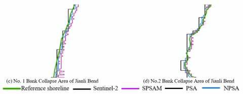
Figure 5. Local magnification and comparison of algorithm results for the No. 1 bank collapse area in Jianli Bend
Figure 6. Local magnification and comparison of algorithm results for the No. 2 bank collapse area in Jianli Bend
It can be seen from the results (see Figure 2, Figure 3, Figure 5, Figure 6) of the above four groups of experiments that the boundary texture through sub-pixel decomposition and location is clear. Under the same scaling, the classification results based on Sentinel 2 image have obvious jagged shape due to the resolution limitation, while the boundary of sub-pixel location results is smooth. Compared with the classification results of the reference image, it can be found that the results obtained by sub-pixel positioning algorithm are closer to the real shoreline curve than those obtained by the original resolution.
By comparing the results of the three sub-pixel positioning algorithms, it can be seen that the three sub-pixel positioning results can improve the resolution of the results to varying degrees, but the SPSAM effect does not show obvious sawtooth, and it is easy to produce some rough “burrs”. Due to the inevitable error in the process of PSA abundance decomposition, more noise is generated. In contrast, NPSA can suppress the noise caused by abundance to a certain extent, and reduce the sensitivity of sub-pixel positioning results to abundance. Especially for the high abundance decomposition error in Jianli bend area, NPSA can still achieve a good sub-pixel mapping effect robustly.
By comparing with the reference results, the commission error and omission error about the water body of each algorithm are obtained, and the overall accuracy is shown in Table 2.
On the whole, SPSAM, PSA and NPSA sub-pixel positioning algorithms can all effectively extract water pixels, and the overall accuracy coefficient can reach a satisfactory level. The specific precision from high to low is NPSA, PSA and SPSAM. On the whole, NPSA is the most effective sub-pixel decomposition algorithm. It can be seen from the analysis of specific categories that the omission error of NPSA water body pixels is the lowest, and the commission error is the highest among the three. The reason is that NPSA combines the classification results of NDWI, so to a certain extent, it inhibits the number of pixel decomposition, thus increasing the number of water body pixels missed, and at the same time, it eliminates some water body sub-pixels on land due to the abundance decomposition error. The results are consistent with the principle of this method.
Table 2. Accuracy of experimental results
|
Study area |
Algorithm |
Commission errors |
Omission errors |
Overall accuracy |
|
Dengpanzhou Bend |
SPSAM |
3.31% |
2.04% |
97.44% |
|
PSA |
2.41% |
2.81% |
97.53% |
|
|
NPSA |
0.61% |
3.63% |
97.99% |
|
|
Jianli Bend |
SPSAM |
9.4% |
0.004% |
96.61% |
|
PSA |
3.60% |
0.07% |
98.62% |
|
|
NPSA |
1.75% |
0.59% |
99.23% |
In this study, we pay more attention to whether the accuracy of shoreline of specific bank collapse area can be improved through sub-pixels, so it is not completely accurate to evaluate only from the perspective of pixels. At the same time, in order to facilitate the comparison of the accuracy of grid data with different resolutions, we further analyze the result accuracy through the changes of specific bank collapse area and surrounding shorelines.
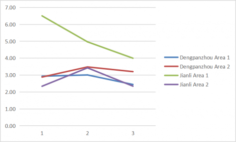
The vector data from the original high-definition reference image or the visual interpretation of the UAV reference image are taken as the shoreline, and the three kinds of water body results are changed into vector boundaries. Figure 7 and Figure 8 are the superposition of the four kinds of boundary extraction results.
In order to avoid the error caused by the processing, the original data of all vectors are raster converted without smoothing. The 0.2-m UAV image is used for the shoreline of Dengpanzhou, and the 1m image of GF2 is used for Jianli Bend to extract the vector boundary directly through visual interpretation. The extracted result is regarded as the real shoreline, and the accuracy of other results is evaluated with RMSE. For the two long-term stable points (house corners, etc.) on the shore in the parallel direction of the shoreline, the verification points shall be selected at a certain interval, and the vertical line shall intersect the extracted shoreline to calculate the distance.
The formula is as follows:
$R M S E=\sqrt{\frac{1}{n} \sum_1^n\left(d_i-D_i\right)^2}$ (10)
where, di is the distance from the verification point to the shoreline extracted by the algorithm; Di is the distance from the verification point to the reference shoreline.
As can be seen from Table 3, the result of SPSAM is relatively the worst. In both Dengpanzhou area 1 and Jianliwan area 1, it is lower than the coastline obtained by the original image of Sentinel 2, so the significance of sub-pixel decomposition is lost in these two areas. Compared with the shoreline extracted in the original classification results, PSA can improve the accuracy of the line to a certain extent, which is generally better than the decomposition results of SPSAM algorithm. However, the RMSE of Jianli bend region 1 is also lower than the original classification accuracy of Sentinel 2 image. NPSA was the optimal value in the three groups of experiments, while in the other group of experiment, it was only inferior to PSA results. In addition, NPSA method was superior to the original image results in all experiments, which was relatively the most robust. There was no case that the accuracy was lower than that before decomposition due to the failure of sub-pixel decomposition.
Table 3. Comparison of results of different algorithms
|
Venue |
Bank Collapse Area |
Algorithm |
RMSE |
|
Dengpanzhou |
Area 1 |
Sentinel-2 |
5.2366 |
|
SPSAM |
3.9304 |
||
|
PSA |
3.8962 |
||
|
NPSA |
2.4427 |
||
|
Area 2 |
Sentinel-2 |
3.5106 |
|
|
SPSAM |
4.2535 |
||
|
PSA |
2.7006 |
||
|
NPSA |
2.9601 |
||
|
Jianliwan |
Area 1 |
Sentinel-2 |
4.5214 |
|
SPSAM |
10.5466 |
||
|
PSA |
5.7548 |
||
|
NPSA |
3.9973 |
||
|
Area 2 |
Sentinel-2 |
4.1628 |
|
|
SPSAM |
3.8087 |
||
|
PSA |
2.7394 |
||
|
NPSA |
2.3454 |
3.4 Discussion
3.4.1 Parameter selection
In the experiment, the exponential parameter of distance and the searching distance for calculating the space gravity are very important parameters. Exponential parameter α is used to measure the importance of distance. For sub-pixel positioning results, too large α and r value will make the water pixel more concentrated, and if α and r value are too small, it is easy to produce broken patterns. For the research scenario in this paper, the accuracy of shoreline prediction results needs to be considered, and it is not easy to analyze whether the clustering or broken pattern caused by α value and r value will exert positive or active impact on the shoreline and obtain definite regularity, and it is generally recommended to test and analyze according to specific images.
The different parameters of this paper are analyzed. Table 4 shows the RMSE results of different α values. α=1, 5, 10, and 15 were used for experiments:
Table 4. Comparison of different α value
|
Area |
Bank collapse area |
α |
RMSE |
Standard deviation |
|
Dengpanzhou |
Area 1 |
1 |
3.0201 |
0.2849 |
|
5 |
3.0487 |
|||
|
10 |
2.4427 |
|||
|
15 |
2.9508 |
|||
|
Area 2 |
1 |
3.3907 |
0.2516 |
|
|
5 |
3.4866 |
|||
|
10 |
2.9601 |
|||
|
15 |
3.0707 |
|||
|
Jianliwan
|
Area 1 |
1 |
4.0246 |
0.2789 |
|
5 |
4.3898 |
|||
|
10 |
3.9973 |
|||
|
15 |
3.7094 |
|||
|
Area 2 |
1 |
3.0801 |
0.3464 |
|
|
5 |
2.8285 |
|||
|
10 |
2.3454 |
|||
|
15 |
3.0801 |
Figure 9. Line chart of different α values
It can be seen from Figure 9 that the values of α has a bottom. When α=10, a fairly good result has been achieved. When α=15, the results in the three areas declined somewhat. Therefore, α=10 is a superior choice.
For the search radius r, a better choice is to make r smaller than the decomposition scale S [6]. Therefore, this paper only considers the r value that is less than the decomposition scale 4. The RMSE calculated from different r values is shown in Table 5.
In this application scenario, r=1 and r=3 both have low RMSE. For the case of r=1, there is a large error in the No.1area of Jianli. Therefore, r=3 is selected for this scenario (As shown in Figure 10).
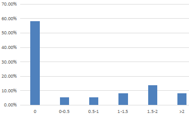
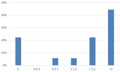
In this paper, the standard deviation is used to measure the fluctuation of results, where the standard deviation of r value is greater than α value in the same area, indicating that the results calculated by different r values fluctuate greatly. Similar results were obtained through analysis of all sample points. As can be seen from Figure 11 (a) above, for different value of α, the standard deviation of more than 50% of the sample points is 0, that is to say, the results of four kinds of parameters calculated for more than 50% of the sample points are consistent, and a total of 92% of the sample points are within the range of 2. The influence of r value is much greater. Figure 11 (b) shows that the sample points larger than 2 are more than 40%. Therefore, it is easier to lower the accuracy of the results if the inappropriate search distance r parameter is selected, so it needs to be taken into account in application.
Table 5. Comparison of different r values
|
Area |
r |
RMSE |
Standard deviation |
|
Dengpanzhou 1 |
1 |
2.9345 |
0.3072 |
|
2 |
3.0075 |
||
|
3 |
2.4427 |
||
|
Dengpanzhou 2 |
1 |
2.8819 |
0.2997 |
|
2 |
3.4807 |
||
|
3 |
3.2033 |
||
|
Jianliwan 1 |
1 |
6.5026 |
1.2634 |
|
2 |
4.9655 |
||
|
3 |
3.9973 |
||
|
Jianliwan 2 |
1 |
2.3393 |
0.6266 |
|
2 |
3.4277 |
||
|
3 |
2.3454 |
Figure 10. Line chart of different r values
(a) Distribution of α value standard deviation
(b) Distribution of r value standard deviation
Figure 11. Distribution of sample point error standard deviation
3.4.2 Application problems
It is easy for the NPSA algorithm to filter out a large amount of noise while filtering out small ponds and pools outside the river area. This is because the segmentation result of the original resolution image is added, causing inevitable information loss. However, in general, these losses have no significant impact on the extraction of the shoreline itself, which is acceptable.
Secondly, in the actual scene, there are many types of artificial surface and riverside soil, and there are many corresponding end element categories, which will affect the solution. As for the type of end element, the type of end element is limited by the number of bands when solving the equation with fully constrained least squares, and based on the consideration of manual workload, a more reasonable choice is to focus on the end element near the river bank.
This paper improves the accuracy of shoreline extraction through pixel positioning, which can better monitor the shoreline erosion, collapse and dynamic changes in the bank collapse area. Among them, the algorithm performance of PSA is improved by constraining the sub-pixel decomposition through dividing NDWI and OTSU. The algorithm experiments were carried out on the bank collapse areas of Dengpanzhou Bend and Jianli Bend in Jingzhou River, and the extraction of image based on Sentinel 2 original resolution, SPSAM extraction, PSA extraction and NDWI+PSA extraction were compared. The results show that both SPSAM and PSA can improve the shoreline extraction accuracy on the whole, but they will produce a lot of noise, especially some shoreline noise is prone to increase the difficulty of shoreline evaluation, and in some application scenarios, the accuracy will decline. NDWI+PSA has good robustness. It can improve shoreline extraction accuracy in a certain extent in multiple scenes, and also remove a lot of noise. It has certain advantages in both visual and quantitative results.
Gratefulness extended to Professor Yu Deqing for providing data and thesis guidance, and to the members of the research team for their inspiration in the process of writing. Here, I would like to express my heartfelt thanks to them all.
Fund: The Open Project of Hunan Provincial Key Laboratory on Remote Sensing Monitoring of Ecological Environment in Dongting Lake Area: “Monitoring of River Bank Collapse in Dongting Lake Area by Combining Multi-platform Remote Sensing Data” (No.: DTH Key Lab.2021-019).
[1] Lai, J.F. (2020). Model test and integrated control technology for river bank collapse in Jiujiang Section of Yangtze River, Nanchang University. https://doi.org/10.27232/d.cnki.gnchu.2020.002098
[2] Zhang, X.N., Jia, D.D., Chen, C.Y. (2021). Features and laws of spatial and temporal distribution of bank collapses in the middle and lower reaches of the Yangtze River. Journal of Basic Science and Engineering, 29(1): 55-63. https://doi.org/10.16058/j.issn.1005-0930.2021.01.005
[3] Zhou, Y.Q. (2005). Study on environmental change of chaohu lake area based on remote sensing. Anhui Normal University, https://doi.org/10.7666/d.D513477
[4] Yang, Z.D., Chen, Y.M., Lu, X.Z., Liu, T.Q., Huang, Y., Zhang, Y.Y. (2010). Remote sensing investigation and study on the changes of bank zone and bank collapse in Anhui Section of the Yangtze River. Remote Sensing for Land & Resources, 2010(S1): 91-97. https://doi.org/10.6046/gtzyyg.2010.s1.21
[5] Yao, Z., Ta, W., Jia, X., Xiao, J. (2011). Bank erosion and accretion along the Ningxia–Inner Mongolia reaches of the Yellow River from 1958 to 2008. Geomorphology, 127(1-2): 99-106. https://doi.org/10.1016/j.geomorph.2010.12.010
[6] Mertens, K.C., De Baets, B., Verbeke, L.P., De Wulf, R.R. (2006). A sub-pixel mapping algorithm based on sub-pixel/pixel spatial attraction models. International Journal of Remote Sensing, 27(15): 3293-3310. https://doi.org/10.1080/01431160500497127
[7] Atkinson, P.M. (2005). Sub-pixel target mapping from soft-classified, remotely sensed imagery. Photogrammetric Engineering & Remote Sensing, 71(7): 839-846. https://doi.org/10.14358/PERS.71.7.839
[8] Tatem, A.J., Lewis, H.G., Atkinson, P.M., Nixon, M.S. (2003). Increasing the spatial resolution of agricultural land cover maps using a Hopfield neural network. International Journal of Geographical Information Science, 17(7): 647-672. https://doi.org/10.1080/1365881031000135519
[9] Chen, L., Wang, T., Zhu, H. (2017). Subpixel Mapping algorithms based on block structural self-similarity learning. Mathematical Problems in Engineering, 2017: Article ID 5254024. https://doi.org/10.1155/2017/5254024
[10] Arun, P.V., Buddhiraju, K.M., Porwal, A. (2018). CNN based sub-pixel mapping for hyperspectral images. Neurocomputing, 311: 51-64. https://doi.org/10.1016/j.neucom.2018.05.051
[11] He, D., Zhong, Y., Wang, X., Zhang, L. (2020). Deep convolutional neural network framework for subpixel mapping. IEEE Transactions on Geoscience and Remote Sensing, 59(11): 9518-9539. https://doi.org/10.1109/TGRS.2020.3032475
[12] Song, M., Zhong, Y., Ma, A., Feng, R. (2019). Multiobjective sparse subpixel mapping for remote sensing imagery. IEEE Transactions on Geoscience and Remote Sensing, 57(7): 4490-4508. https://doi.org/10.1109/TGRS.2019.2891354
[13] Zhang, N., Wang, P., Sang, H.Y., Yan, H.Y., Zhai, L. (2019). Sub-pixel mapping of flood inundation from MODIS data science of surveying and mapping. Mapping Science, 44(02): 164-170. https://doi.org/10.16251/j.cnki.1009-2307.2019.02.026
[14] He, B.T. (2009). Research on MODIS water extraction model and method based on sub-pixel decomposition and reconstruction. Huazhong University of Science and Technology, https://doi.org/10.7666/d.d088161
[15] Huang, C., Chen, Y., Wu, J. (2013). A DEM-based modified pixel swapping algorithm for floodplain inundation mapping at subpixel scale. In 2013 IEEE International Geoscience and Remote Sensing Symposium-IGARSS, pp. 3994-3997. https://doi.org/10.1109/IGARSS.2013.6723708
[16] Hong, Z., Li, X., Han, Y., Zhang, Y., Wang, J., Zhou, R., Hu, K. (2019). Automatic sub-pixel coastline extraction based on spectral mixture analysis using EO-1 Hyperion data. Frontiers of Earth Science, 13(3): 478-494. https://doi.org/10.1007/s11707-018-0702-5
[17] Adams, J.B., Smith, M.O., Johnson, P.E. (1986). Spectral mixture modeling: A new analysis of rock and soil types at the Viking Lander 1 site. Journal of Geophysical Research: Solid Earth, 91(B8): 8098-8112. https://doi.org/10.1029/JB091iB08p08098
[18] Shimabukuro, Y.E., Smith, J.A. (1991). The least-squares mixing models to generate fraction images derived from remote sensing multispectral data. IEEE Transactions on Geoscience and Remote sensing, 29(1): 16-20. https://doi.org/10.1109/36.103288
[19] Otsu, N. (1978). A thresholding selection method from gray-level histogram. IEEE SMC-8, pp62-66. OSTU N. A Thresholding Selection Method from Gray Level Histogram. IEEE SMC-8, 1978: 62-66.