Dilber Çetintaş* | Taner Tuncer
© 2022 IIETA. This article is published by IIETA and is licensed under the CC BY 4.0 license (http://creativecommons.org/licenses/by/4.0/).
OPEN ACCESS
By examining the change of eye movements during reading, it is possible to determine the type of document read. Returning to the previous position (negative saccade), blink, fixation, and position are important indicators in determining the type of document being read. In this paper, a hybrid deep learning model is proposed to determine the type of document read. The MPIIDPEye dataset, which includes eye movement data of 10-minute comic, newspaper and text document readings from 20 participants, was used. First, the eye movements obtained over time were augmented by the non-linear interpolation technique. In order to process the data of each class with convolutional neural network, spectrogram images of the signals were created. Spectrogram images were given as input to Resnet architectures and the features in the Fc1000 layer were combined. Concatenated feature vectors were given as an input to feature selection algorithms. The most effective features in classification accuracy were determined and classified using the SVM algorithm. The classification was carried out for 3 different cases, and the highest accuracy of 98.41% was obtained for case-2, where Fixation, Position, and Blink properties were used.
eye-tracking, fixation, blink, saccade, convolutional neural network
Eye-tracking technology, together with hardware and software developments, allows the collection of features such as focusing, saccade, and blinking from the user. These data are widely used in sciences such as health, psychology and education and help to obtain information about people. For example, a student with distraction or reading difficulties is likely to identify his/her condition in the early stages. Cognitive processes such as letter recognition, distinguishing by solving the connection between letters, word recognition and understanding the meaning of the word, which occur in the brain during reading, are directly related to eye movements [1]. Eye movements during reading can be accessed by fixed eye-tracking devices [1, 2], which are generally adapted to a monitor to be used in a certain place. Thanks to eye-tracking technology, many features such as focusing time, pupil sizes for left and right, coordinates of the focused point, number of blinks and duration can be obtained. Analyzing these values, which can be taken numerically or visually, allows important inferences to be made about the user.
A study of users' visual attention based on eye movements of users viewing web pages with different designs was reported by Sutcliffe and Namoun [3]. The effect of web page layout on visual attention and how it affects anchoring patterns for browsing and searching is shown. An eye-tracking experiment was conducted to examine the hypothesis that subjects who care about the product selection criteria in an advertisement's message pay more attention to the message than those who don't. Eye-tracking data was collected by showing 81 college students ads and websites with the messages "reduces body fat", "low in calories", and "good for dieting". Associated with eye-tracking data on websites where subjects changed their attentional disposition. In studies using 4 different brands of beverages with different calorie values, it was observed that there were differences in fixation times between low-calorie and high-calorie beverages. It was concluded that the fixation time was longer on texts claimed to be beneficial for diet [4]. In which the driver's focus is tried to be found, a data set containing more than 500000 frames are created with the camera attached to the vehicle and the glasses given to the driver [5]. The aim is to predict what a person will pay attention to while driving and which part of the scene around the vehicle is more mission-critical. The results discovered that one of the most important factors in driver attention is experience, and changing environment, light, and weather conditions affect attention. It was stated that the most effective factor on attention was saccade. Ross et al. studied the effect of music on eye movements. Tracking position, fixation, and saccade were compared for slow-moving targets and fast-moving targets, first without music and then with music. There was a significant difference between position and saccadic features in slow tempo, both no-music and musical conditions. In fast tempo, a significant difference was found between the fixation time and saccadic characteristics in both no-music and musical conditions. These results point to the positive effect of music intervention on the pre-motor and motor ocular systems, revealing its effect on visual attention in different tempos. In the absence of music, focus time and saccadic gain show success at similar rates, while in the case of music use, these success rates decrease, and when the tempo is increased, success decreases at a higher rate. It provides evidence of how different musical tempos affect visual cognition in children. The significance of the study is that it adds to and expands existing knowledge of research on children's eye movement tracking by comparing two distinct types of vision targets at different tempos (adagio and allegro), first without music and then with music. This study is part of a larger project examining the tracking and saccadic eye movement patterns of children with autism and how specific musical pitches embedded in targets stimulate attention, concentration and visual fixation in children with learning disabilities. The results of the study also contributed to the creation of specially composed music that was later applied in sensory integration therapy for children with autism [6].
One of the characteristic features of autism spectrum disorder (ASD) is difficulty making or maintaining eye contact. Carette et al. proposed a methodology for visualizing the eye-tracking patterns of individuals with ASD, focusing on children in the early stages of development. Features such as eye focus position on the screen, Eye position in space, Pupil dilation, Fixation, and saccade were used. According to the results obtained, it was emphasized that the diagnosis of developmental disorders can be made with eye-tracking technology [7].
Inoue et al. examined how fluent and non-fluent readers process text and images using eye movement methodology. By examining eye movements, it was observed that the concentration level of good readers was better. Good readers had a wider field of view, while poor readers had a narrower field of view. The most obvious difference between the two was that poor readers could not understand a text by looking at it, and poor readers spent a significant amount of time [8]. When the relationship between mind and blinking was sought during the reading task, it was noticed that the number and duration of blinks varied according to the stimulus/task interaction [9]. Longer blinks on less interesting tasks confirmed the study's hypothesis. Recommendations are presented for researchers who want to accurately derive blink events from continuous, binocular, eye-tracking data.
Ahrens et al. used eye-tracking to record and divert developers' attention during software maintenance. It was aimed to color the codes written in Java language and enable developers to reach the relevant area faster. Although colorings reduce cognitive load, it has been found that developers, especially experienced ones, have attention problems. It was also found that the Saccade number is a good indicator of the relevance of an episode in the context of software maintenance [10].
Arsenovic et al. proposed a new deep learning-based architecture for the eye movement classification task. The proposed architecture is an aggregated approach using deep convolutional neural networks operating in parallel for both eyes separately for visual feature extraction and recurrent layers for temporal information collection. For training and validation, dataset images were collected from a standard webcam and preprocessed automatically using special tools. The overall accuracy of the improved classifier in the validation set was 92%. The overall accuracy in real-time tests was 88% [11].
Al-gawwam and Benaissa used SVM, Adaptive Boost (AdaBoost), Naive Bayes, and Bagging classifiers to reveal the relationship between blinking and depression. They observed that the depressive patient group, whose understanding requires serious clinical experience, performed more blinking movements than the control group. The best results were achieved with the Adaboost classifier, and as a result of the findings, it was observed that depressed people blinked longer and the number of blinks increased as they improved. These findings can be a sign of fatigue, which is an indicator of depression, as well as an indicator of distraction [12].
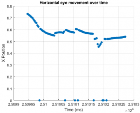
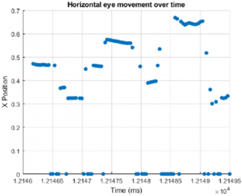
Figure 1. Comic, newspaper, and text position(x)-time change, respectively
Wang et al. performed biometric recognition by eye movement based on the principle that human eye movements when reading text are different between individuals but are constant for a particular individual. A deep learning framework was proposed to assess fixation sequence similarity and a computational model for eye-movement recognition was constructed. Biometric recognition accuracy was 85.4% [13].
Bachurina et al. examined the mental attention capacities of users who tried the Color Matching Task at six different difficulty levels. They presented machine learning methods that take into account measures of task difficulty, reaction time, and eye movement. The results showed that the machine learning models were able to predict performance robustly, with reaction times and difficulty level being the strongest predictors. The accuracy of fixation number, saccade number, available fixation time, and pupil size were independently estimated from eye-tracking indices [14].
1.1 Motivation
Returning to the previous position (negative saccade), blinking, fixation, and position are important indicators in determining and understanding the type of document read. For example, comparing the position of the eye movement of the individual at the time of t and t+1 during reading indicates whether the type of document being read is understood or whether there is a distraction. If the x position at time t+1 goes backward from its position at time t (negative saccade), it is concluded that the text read was not understood. In Figure 1, x positions are given against time while the same user is reading comedy, newspaper, and text documents. These images were drawn by taking 100 eye movements from the start.
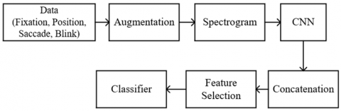
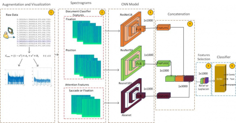
In Figure 1, the horizontal axis indicates the time, while the vertical axis gives the coordinate value of the x point of the eye looking at the monitor. As it can be seen in the figure, the negative saccade movement occurs at least in the comic document and mostly in the text document. Especially in the text type, too much rotation to the starting point (x=0) takes place. In this paper, it has been determined whether features such as negative saccade, blink, fixation and position can be used in determining the type of document read. With the use of these features together, the determination of the type of document read is provided with high accuracy. The proposed method consists of augmentation, spectrogram, CNN model, Concatenation, feature selection and classification stages. The graphical outline of the proposed method is shown in Figure 2.
Figure 2. The block diagram of the proposed method
1.2 Innovations and contributions
- Linear interpolation data augmenting method was applied to each feature in the data set.
- The feature vectors obtained from ResNet architectures were concatenated and a new feature vector was created to determine the document type.
- The feature selection algorithms were used to determine the most dominant features in determining the document type.
- In addition to fixation and position features, saccade and blink eye features, which are important in determining distraction, were also taken into account in the classification.
In this study, the MPIIDPEye [15] dataset containing eye movement data of a total of 20 users, 10 male, and 10 female, was used. The data set was obtained from participants between the ages of 21 and 45. Users were made to read documents in different types of comics, newspapers, and texts, which contain different percentages of visuals. A maximum reading time of 10 minutes was determined for each type. This period varies according to the participant's reading skill. Eye movements of the participants were recorded as a video and no calibration was performed before recording. Not all participants had experience with eye-tracking exercises, and participants were encouraged to read at their usual pace. In the creation of the dataset, the participants did not know what was measured in this activity. After reading the document, 52 feature datasets were created for each participant. In this study, negative saccade, fixation, position, and blink features in the data set were used. The data were divided into 67% training, and 33% test respectively.
2.1 Fixation
Fixation is the condition where the eye stays focused on a certain point. Fixation specifies what the object is and where it is in space. An increase in the fixation time indicates that there is deeper processing or that it is directed to the field of personal interest. When evaluated with ANOVA by taking eye characteristics such as saccade, fixation number, fixation time in a study conducted to predict consumer decisions, the results show that fixation numbers and total fixation time largely predict the consumer's decision [16]. In a machine learning study for emotion classification, only fixation and pupil features are used and as a result of classification with the Support Vector Machine algorithm, 75% accuracy is achieved with fixation, while 57% success rate is achieved with pupil [17].
2.2 Saccade
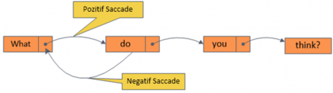
In order for the images in the field of view to be perceived and mapped in the mind, the eye has to constantly move. This is because only the fovea region of the retina perceives it with high acuity. The jumping of both eyes from one point to another together is called a saccade. Saccade duration and width vary depending on the distance between points. As seen in Figure 3, the jump made in the forward direction is called the positive saccade, and the jump made in the reverse direction is called the negative saccade. This feature is an effective indicator of the complexity or distraction of the text [18]. It is detailed in the study of Özer and Özdemir [19] that the reading efficiency decreases as the saccade increase.
2.3 Blink
The anterior part of the cornea is covered with a thin liquid film called the "precorneal tear film". The eyelids need to be opened and closed regularly to spread this tear fluid across the corneal surface. The average blink rate ranges from 12 to 19 cycles per minute at rest [20]; it is affected by environmental factors (e.g., relative humidity, temperature, brightness) as well as physical activity, cognitive workload, or fatigue [21]. As the reading time increases, the blink count starts to increase. This is an indication that the document read is complex or that the document cannot be understood.
2.4 Position
It contains the coordinates of the point where the pupils look during gaze. Since the eyes move from left to right during reading, it is expected to show an increasing trend in the x coordinate. Decrease or repetition of this situation after reaching a certain point indicates that the document read is not understood.
Figure 3. Positive and negative eye saccade movement
In this study, Fixation, position, Blink and Saccade properties were used to determine the type of document read. The flowchart and detailed block diagram of the model developed for this purpose are given in Figure 4 and Figure 5.
The method consists of six subunits. These are augmentation and visualization, Spectrogram, Deep learning, concatenation, feature selection and classification, respectively.
With the proposed model, document classification is completed with a 6-step process.
Step 1: Augmentation from fixation, position, saccade or blink raw signals with linear interpolation method: One of the 20 user-owned features kept in csv format is discussed. The users' values for this property are used for multiplexing. Using the formula specified in Eq. (1), (9) more new data are generated from two consecutive users. A signal graph of each generated value against time is created.
Step 2: Obtain the spectrogram image for each signal: The data in our dataset contains numerical values. In order to make these values more understandable, visuals are created with the spectrogram technique. This technique is obtained by splitting the signals into parts or frames and performing the Fourier transform.
Step 3: Give spectrogram images as input to ResNet architectures. Obtain feature vectors from the fc1000 layer of ResNet architectures: It is given as input value to fixation and position which have focusing properties and saccade and blink Resnet architectures which have attention properties. Before these properties are given as input, three different combinations are determined. These combinations are Case 1: Fixation+Position, Case 2: Fixation+Position+Saccade, Case 3: Fixation+Position+Blink.
Figure 4. The flowchart of the proposed model
Figure 5. The proposed method
Step 4: Concatenate the feature vectors: The 1x1000 dimensional vectors obtained from each model are combined to form a 1x3000 sized feature vector.
Step 5: Select the features with the highest classification accuracy from the concatenate feature vector with feature selection algorithms: Laplacian and Relief algorithms are preferred for feature selection.
Step 6: Classify the feature vectors with the SVM classifier.
Details of each step used for classification are as follows.
Step 1: Non-linear augmentation and visualization
Nonlinear interpolation is a curve fitting method that uses nonlinear polynomials to generate new data from known points. Data augmentation methods, in which new time series are obtained from an interpolated time series, are available in the literature [22, 23]. The data set to MPIIDPEYE was created with the participation of 20 users and the number of data obtained as a result of augmenting are given in Table 1. 209 new data were generated from the data set in each class.
Table 1. Number of data before and after augmenting
|
|
Comic |
Newspaper |
Text |
|
MPIIDPEye |
20 |
20 |
20 |
|
Augmented |
209 |
209 |
209 |
As seen in the table, 20 data numbers belonging to each document at the beginning were obtained as 209 as a result of interpolation. Eq. (1) was used to augment these data with the non-linear interpolation technique.
$C_{\text {new }}(t)=\left(1-u^2\right) \times A(t)+u^2 \times B(t) \quad 0 \leq \mathrm{u} \leq 1$ (1)
where, A and B represent any eye movement data of the two participants, and Cnew is the new data obtained for the incremental value of u. For example; Let the fixation change of two participants A and B be as follows:
A(t)=[0.17, 0.25, 0.48,…]
B(t)=[0.82, 0.72, 0.22, …]
If u=0.4, according to Eq. (1), Cnew(t) is obtained as follows.
Cnew(t)=[0.27, 0.33, 0.44,…]
A(t) is obtained for u=0 and B(t) is obtained for u=1.0. When the increment value is u=0.1, 9 new data are generated from participants A(t) and B(t). The data number is obtained as 209(21x9+20) for 21 binary users randomly selected from 20 participants.
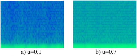
Step 2: Obtaining the spectrogram images
Automatic feature extraction is to automatically extract features from signals or images without the need for hunches. It is standard to use special algorithms or deep networks for this. In this paper, it was preferred to convert the signals to images in order to extract features from the eye signals. Generally preferred visualization methods are heatmap and gaze plot. Unlike these, in the study, eye signals were converted to spectrogram images. A spectrogram is a visual way of representing the signal strength or "height" of a signal over time at the various frequencies available in a given waveform. The function to be converted is multiplied by a nonzero window function. The window is scrolled along the time axis. The Fourier transform of the resulting signal is taken and a two-dimensional representation of the signal is created. Mathematically, this is written as [23]:
$\operatorname{STFT}\{x(t)\}(\tau, \omega) \equiv X(\tau, \omega)$$=\int_{-\infty}^{\infty} x(t) w(t-\tau) e^{-i \omega t} d t$ (2)
where, x[n] and w[n] denote the signal and the window function, respectively. X(τ,ω) is essentially the Fourier transform of x(t)w(t-τ), representing the phase and magnitude of the signal over time and frequency. Figure 6 shows the spectrogram images obtained from the fixation signal for the 0.1 and 0.7 values of u.
The size of the images is 227x227x3 for feeding the obtained spectrogram images into the ResNet models.
Figure 6. Spectrogram images for fixation
Table 2. ResNet18, ResNet50 and ResNet101 model architecture
|
Layer |
18 – layer |
50 – layer |
101 – layer |
|
Conv1 |
7 x 7,64,stride2 |
||
|
Conv2_x |
3x3 maxpool,stride2 |
||
|
$\left[\begin{array}{lll}3 & x & 3,64 \\ 3 & x & 3,64\end{array}\right] \mathrm{x} 2$ |
$\left[\begin{array}{ccc}1 & x & 1,64 \\ 3 & x & 3,64 \\ 1 & x & 1,256\end{array}\right] \mathrm{x} 3$ |
$\left[\begin{array}{ccc}1 & x & 1,64 \\ 3 & x & 3,64 \\ 1 & x & 1,256\end{array}\right] \mathrm{x} 3$ |
|
|
Conv3_x |
$\left[\begin{array}{lll}3 & x & 3,128 \\ 3 & x & 3,125\end{array}\right] \mathrm{x} 2$ |
$\left[\begin{array}{ccc}1 & x & 1,128 \\ 3 & x & 3,128 \\ 1 & x & 1,512\end{array}\right] \mathrm{x} 4$ |
$\left[\begin{array}{ccc}1 & x & 1,128 \\ 3 & x & 3,128 \\ 1 & x & 1,512\end{array}\right] \mathrm{x} 4$ |
|
Conv4_x |
$\left[\begin{array}{lll}3 & x & 3,256 \\ 3 & x & 3,256\end{array}\right] \mathrm{x} 2$ |
$\left[\begin{array}{ccc}1 & x & 1,256 \\ 3 & x & 3,256 \\ 1 & x & 1,1024\end{array}\right] \mathrm{x} 6$ |
$\left[\begin{array}{ccc}1 & x & 1,256 \\ 3 & x & 3,256 \\ 1 & x & 1,1024\end{array}\right] \mathrm{x} 23$ |
|
Conv5_x |
$\left[\begin{array}{lll}3 & x & 3,512 \\ 3 & x & 3,512\end{array}\right] \mathrm{x} 2$ |
$\left[\begin{array}{ccc}1 & x & 1,512 \\ 3 & x & 3,512 \\ 1 & x & 1,2048\end{array}\right] \mathrm{x} 3$ |
$\left[\begin{array}{ccc}1 & x & 1,512 \\ 3 & x & 3,512 \\ 1 & x & 1,2048\end{array}\right] \mathrm{x} 3$ |
Step 3: Deep learning model and feature extraction
Deep learning-focused models have recently proven successful in many clinical applications [24, 25]. These models provide better feature extraction than manually extracted features and traditional mathematical models in medical image processing and machine vision. The most important feature that distinguishes deep learning architectures from traditional artificial neural network models is that the layers within the deep networks can extract the feature map of the data. Thanks to these architectures, feature extraction is provided by applying filters in different sizes and numbers in the data. ResNet18, ResNet50, and ResNet101 were used as feature extractors in this paper. The most different one among the optimizations and innovations made in Deep Networks is the ResNet architecture, where 'residual' connections are made [26]. Table 2 shows the architecture of the ResNet models.
In this paper, fixation, position, saccade and blink properties were evaluated from the 52-featured dataset of the participants during the reading process, and the type of document read was determined. The spectrogram images created in the second step were fed into the ResNet models. The size of the feature vector obtained from the fc1000 layer for each model is 1x1000. The mathematical definition for combining the obtained feature vectors and obtaining the 1x3000 dimensional feature vector is as follows.
Let Ifixation, Iposition, Isaccade display spectrogram images. By feeding these images to the ResNet models, the feature vectors in the fc1000 layer are obtained, respectively,Ffixation, Fposition, Fsaccade.
Ffixation=ResNet18(Ifixation)
Fposition=ResNet50(Iposition)
Fsaccade=ResNet101(Isaccade)
Step 4: Concatenating feature vectors
The resulting feature vectors of 1x1000 are subjected to the concatenate function. Thus, a concatenated feature vector F of 1x3000 is obtained. where, | is the concatenation operator.
F= Ffixation | Fposition| Fsaccade (3)
Step 5: Feature selection
Feature selection is defined as the selection of the best subset that can represent the original dataset. In this paper, Laplacian and ReliefF feature selection algorithms are used to select the best features from the concatenated feature vector.
Laplacian Score: LS is based on the observation that two data points that are close to each other are probably related to the same class [27]. For any data point, the distance (Di, j) is calculated using the nearest neighbor method. The distance is converted into the similarity matrix (Eq. (4)) using the kernel function.
$S_{i, j}=\exp \left(-\left(\frac{D_{i, j}}{\sigma}\right)^2\right)$ (4)
where, σ denotes the scale factor for the kernel function.
The Laplacian score is determined with the help of the equation by calculating the mean ($\tilde{x}_r$) and score (Sr) for each feature.
$\tilde{x}_r=x_r-\frac{x_r^T D_g \mathbf{1}}{\mathbf{1}^T D_g \mathbf{1}}$ (5)
where, xr is the rth feature, Dg is the degree matrix, and 1T=[1,⋯,1]T.
$S_r=\frac{\tilde{x}_r^T S \tilde{x}_r}{\tilde{x}_r^T D_g \tilde{x}_r}$ (6)
$L_r=1-\frac{\tilde{x}_r^T S \tilde{x}_r}{\tilde{x}_r^T D_g \tilde{x}_r}$ (7)
L is the Laplacian matrix, defined as the difference between Dg and S.
ReliefF: The ReliefF algorithm is a feature selection method that calculates the weight values of the features according to the relationship between the features [28]. First, the closest feature values for each class are determined. After calculating the weight of the features, the features are ranked according to their weights. Finally, the best k features are selected. The pseudo-code of the ReliefF algorithm is given in Algorithm 1.
Algorithm 1. Pseudo-code of the ReliefF algorithm
|
Input: a vector of feature values and class value |
|
Output: calculation of weights and selection of k |
|
1. Set all weights W[X]:=0.0; 2. for i:= 1 to m 3. Randomly select an sample Ri 4. Find k nearest hits Hj 5. for each class Cǂ class(Ri) 6. From class C find k nearest missed Mj(C) 7. for X:= 1 to n 8. $W[X]:=W[X]-\sum_{j=1}^k \operatorname{diff}\left(X, R_i, H_j\right) /(m . k)$$+$ $\sum_{c \neq \operatorname{class}\left(R_i\right)} \frac{P(c)}{1-P\left(\operatorname{class}\left(R_i\right)\right)} \sum_{j=1}^k \operatorname{diff}\left(X, R_i, M_j(C)\right) /(m . k)$ 9. end |
Here, $W$ represents the weight (significance) of the $\mathrm{j}^{\text {th }}$ feature, $H_{\mathrm{j}}$ is the relevant feature value in the closest sample with the same class, and $M_{\mathrm{j}}$ is the related feature value in the closest sample with a different class. The diff function calculates distances between samples and features (Eq. (8)). $I_1$ and $I_2$ are samples, $X$ is a feature.
$\operatorname{diff}\left(X, I_1, I_2\right)=\frac{\mid \text { value }\left(X, I_1\right)-\operatorname{value}\left(X, I_2\right) \mid}{\max (X)-\min (X)}$ (8)
Step 6: Classification
The last stage is the classification stage and the support vector machine was used as a classifier. The support vector machine method is based on estimating the most appropriate function to separate the data from each other [29]. SVM performs classification with the aid of a linear or nonlinear function. The goal is to obtain the optimal separation hyperplane that will separate the classes from each other. In other words, it is to maximize the distance between support vectors belonging to different classes [30-32].
In this study, three cases were examined to classify the type of comic book, newspaper, and text document read by the participants. In Case-1, negative saccade, blink, fixation, and position properties obtained from the participants were used separately and classified with pre-trained ResNet architectures. In Case-2, the fixation, position, and blink properties were given as input to the Resnet18, ResNet50 and ResNet 101 models, and classification was carried out with the proposed model. Unlike Case-2, the negative Saccade was used instead of the blink given to the Resnet101 model input in Case-3.
Accuracy, precision, recall, F1-score, and misclassification rate parameters obtained from the confusion matrix were used to determine the classification performance for all three cases. To calculate these performance metrics, the true number of positives (tp), the number of true negatives (tn), the number of false positives (fp), and the number of false negatives (fn) are used for each class. The mathematical equations of the performance parameters are given below.
$\operatorname{Accuracy}(A)=\frac{\mathrm{tp}+\mathrm{tn}}{\mathrm{tp}+\mathrm{tn}+\mathrm{fp}+\mathrm{fn}}$
Precision $(P)=\frac{\mathrm{tp}}{\mathrm{tp}+\mathrm{fp}}$
$\operatorname{Recall}(R)=\frac{\mathrm{tp}}{\mathrm{tp}+\mathrm{fn}}$ (9)
$F 1 \operatorname{Score}(F 1)=\frac{2 \mathrm{tp}}{2 \mathrm{tp}+\mathrm{fp}+\mathrm{fn}}$
Misclassification rate $(M R)=\frac{\mathrm{fp}+\mathrm{fn}}{\mathrm{tp}+\mathrm{tn}+\mathrm{fp}+\mathrm{fn}}$
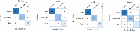
Case-1: fixation, position, negative saccade, and blink signals were classified separately with ResNet models. The confusion matrix obtained as a result of this classification is as in Figure 7. The models with the highest accuracy in the classification of Fixation, Position, Blink, and Saccade properties are ResNet18, ResNet50, ResNet101, and ResNet101, respectively. The average accuracy values obtained are 98.14%, 93.12%, 96.83% and 95.77%, respectively, and the performance parameters according to the classes are as in Table 3. The misclassification rate, which indicates the percentage of incorrect predictions, is 5.3%, 6.2%, 2.9% and 3.8%, respectively
The model in Figure 5 is proposed to achieve higher classification accuracy. The accuracy of the model was examined for case-2 and case-3.
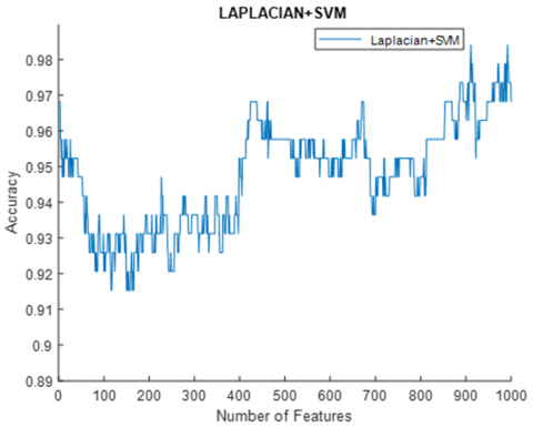
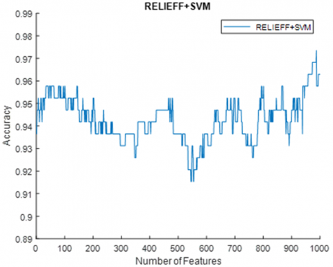
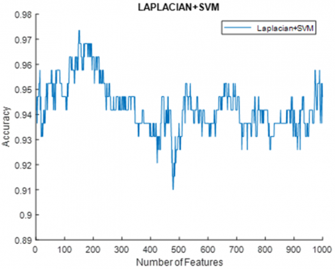
Case-2: Fixation, Position, and Blink signals were fed to ResNet18, Resnet50, and Resnet101 models, respectively. The feature vector formed by concatenating the features obtained from the Fc8 layer is given to the feature selection algorithms. With the help of the feature selection algorithm, the ranks of the features are determined. Among these features, the features that maximize the classification accuracy are selected. With the Laplacian algorithm used for feature selection, maximum accuracy was obtained when the first 911 features of the feature vector ordered according to their rank were used. The classification accuracy obtained was 98.41%. In the case of using the ReliefF algorithm, the maximum accuracy was 97.35% with the use of the first 987 features (Figure 8). The lowest misclassification rate was 1.43%. Table 4 shows the values of the performance parameters obtained according to the classes for case-2.
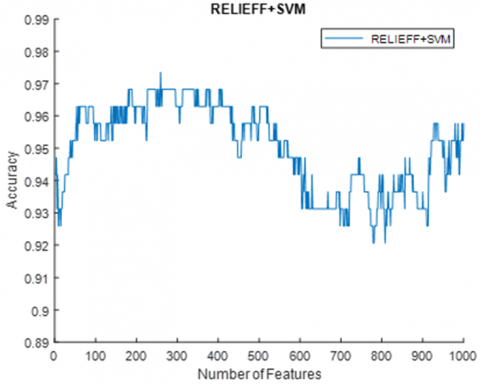
Case-3: Unlike Case-2, Saccade was used instead of Blink in this case. Using the Laplacian and ReliefF feature selection algorithms, the feature vectors were sorted separately according to their rank. Maximum accuracy was obtained by using the first 259 features of the feature vector obtained by the Laplacian algorithm. Maximum accuracy was achieved in the first 150 features with the ReliefF algorithm. The accuracy value obtained for both cases was 97.35% (Figure 9). The calculated misclassification rate value was 2.4%. Table 5 shows the values of the performance parameters obtained for Case-3.
Figure 7. Confusion matrices for Case-1
Table 3. Performance parameters for Case-1
|
|
Resnet18 (Fixation) |
Resnet50(Position) |
||||||
|
|
A(%) |
P(%) |
R(%) |
F1(%) |
A(%) |
P(%) |
R(%) |
F1(%) |
|
Comic |
97.35 |
98.41 |
93.94 |
96.12 |
96.83 |
93.85 |
96.83 |
95.31 |
|
Newspaper |
94.71 |
92.06 |
92.06 |
92.06 |
94.18 |
91.94 |
90.47 |
91.24 |
|
Text |
96.3 |
92.06 |
96.67 |
94.30 |
95.24 |
93.55 |
92.06 |
92.79 |
|
|
Resnet101 (Blink) |
Resnet101(Saccade) |
||||||
|
|
A(%) |
P(%) |
R(%) |
F1(%) |
A(%) |
P(%) |
R(%) |
F1(%) |
|
Comic |
100 |
100 |
100 |
100 |
98.41 |
98.41 |
96.87 |
97.63 |
|
Newspaper |
96.83 |
98.41 |
92.54 |
95.38 |
96.3 |
95.29 |
93.75 |
94.51 |
|
Text |
96.83 |
92.06 |
98.31 |
95.08 |
96.84 |
93.65 |
96.72 |
95.16 |
Table 4. Performance parameters for Case-2
|
|
Laplacian |
Relieff |
||||||
|
|
A(%) |
P(%) |
R(%) |
F1(%) |
A(%) |
P(%) |
R(%) |
F1(%) |
|
Comic |
98.94 |
98.41 |
98.41 |
98.41 |
98.41 |
96.83 |
98.38 |
97.59 |
|
Newspaper |
98.94 |
98.41 |
100 |
99.19 |
98.94 |
96.83 |
100 |
98.38 |
|
Text |
99.47 |
98.41 |
96.87 |
97.63 |
97.35 |
98.41 |
93.94 |
96.12 |
Table 5. Performance parameters for Case-3
|
|
Laplacian |
Relieff |
||||||
|
|
A(%) |
P(%) |
R(%) |
F1(%) |
A(%) |
P(%) |
R(%) |
F1(%) |
|
Comic |
98.41 |
98.41 |
96.87 |
97.63 |
97.88 |
98.41 |
95.38 |
96.87 |
|
Newspaper |
97.88 |
96.83 |
96.83 |
96,83 |
98.41 |
96.83 |
100 |
98.38 |
|
Text |
98.41 |
96.83 |
98.38 |
97.59 |
98.41 |
96.83 |
96.83 |
96.83 |
a) Laplacian
b) ReliefF
Figure 8. Accuracy change according to the features used (case-2)
When all properties were evaluated separately in line with the findings obtained, it was determined that successful classification was performed with the blink property. It was observed that the classification success rate increased even more for case-2 and 3 with attention markers. The highest classification accuracy was achieved with the Fixation, position, and blink properties considered in the second scenario. Instead of 3000 features created by concatenating the feature vector, 1000 features were selected. Thus, faster and higher classification accuracy was achieved. Among the document types, the most successful results were obtained in the field of comics. This result is due to the fact that the comedy document contains more visual images and the focus is higher. The highest rates in the comics document and the lowest in the text document reflect the strong link between visual imagery, attention, and focus. The study shows that the properties that affect attention make a positive contribution to the finding of document differences.
The limitation of this study is that the results obtained cannot be compared with the literature due to the limited data set on eye movements in the literature.
a) Laplacian
b) Laplacian
Figure 9. Accuracy change according to the features used (case-3)
In this paper, document classification was performed with a hybrid model developed with the use of ResNet18, ResNet50, and ResNet101 architectures. Firstly, data augmenting was performed to eliminate the lack of data. Fixation, position, negative saccade, and blink signals were augmented with non-linear interpolation and then converted to spectrogram images. Three scenarios (Case-1, Case-2, Case-3) were examined to demonstrate that documents could be classified from the eye signals used. In Case 1, each feature was evaluated separately. The highest accuracy was obtained with the ResNet101 model using the blink in this scenario. Fixation, position, blink in Case 2, fixation, position, and negative saccade properties in Case 3 were used. 3000 features formed by concatenating the feature vectors were given to the Laplacian and ReliefF feature selection separately, and the features that maximized the classification accuracy were selected. The highest success rate was obtained with Laplacian as 98.41% in the Case-2 scenario. We foresee that the proposed model and the fixation, position, blink, and saccade can be used in subjects such as distraction, determining user interests, and determining the level of reading skill. Another important advantage of the study is the successful application of the non-linear interpolation method to the insufficient number of signal data. As a result, our study is a pioneering study in document classification.
This study proves that some results can be achieved while doing our daily work in front of a screen. Eye defects can be detected by eye movements while users are reading the newspaper, or information about behavioral characteristics can be obtained while shopping online. In fact, autism can be caught early by measuring the attention levels of child users.
Devices used to acquire eye-tracking data are costly and time-consuming. For this reason, studies are always trying to reach a result with a limited number of users. It has been shown that the data can be used by increasing the nonlinear interpolation process. In order to visualize the numerical values obtained in the eye tracking field, heat map, gaze graph and focus map techniques were used in the studies. Unlike these approaches, a new visualization method has been introduced to the field of eye tracking by using the spectrogram technique in the paper.
[1] Rayner, K., Pollatsek, A., Ashby, J., Clifton Jr, C. (2012). Psychology of Reading. Psychology Press. https://doi.org/10.4324/9780203155158
[2] Özer, E., Özdemir, S. (2021). Okuma araştırmalarında geçmişten günümüze göz izleme tekniği. Ankara Üniversitesi Eğitim Bilimleri Fakültesi Özel Eğitim Dergisi.
[3] Sutcliffe, A., Namoun, A. (2012). Predicting user attention in complex web pages. Behaviour & Information Technology, 31(7): 679-695. https://doi.org/10.1080/0144929X.2012.692101
[4] Okano, M., Asakawa, M. (2017). Eye tracking analysis of consumer's attention to the product message of web advertisements and TV commercials. In 2017 5th International Conference on Cyber and IT Service Management (CITSM), pp. 1-5. https://doi.org/10.1109/CITSM.2017.8089270
[5] Palazzi, A., Abati, D., Solera, F., Cucchiara, R. (2018). Predicting the driver's focus of attention: The DR (eye) VE project. IEEE Transactions on Pattern Analysis and Machine Intelligence, 41(7): 1720-1733. https://doi.org/10.1109/TPAMI.2018.2845370
[6] Ross, V., Rosli, S.A., Rudin, A.M.A., Buari, N.H., Ahmad, A., Chen, A.H. (2015). Pursuit position gain, fixation duration and saccadic gain with music intervention in eye motion tracking. In 2015 SAI Intelligent Systems Conference (IntelliSys), pp. 818-821. https://doi.org/10.1109/IntelliSys.2015.7361236
[7] Carette, R., Elbattah, M., Dequen, G., Guérin, J.L., Cilia, F. (2018). Visualization of eye-tracking patterns in autism spectrum disorder: Method and dataset. In 2018 Thirteenth International Conference on Digital Information Management (ICDIM), pp. 248-253. https://doi.org/10.1109/ICDIM.2018.8846967
[8] Inoue, A., Paracha, S. (2016). Identifying reading disorders via eye-tracking technology. In 2016 International Conference on Advanced Materials for Science and Engineering (ICAMSE), pp. 607-610. https://doi.org/10.1109/ICAMSE.2016.7840213
[9] Rahal, R.M., Fiedler, S. (2019). Understanding cognitive and affective mechanisms in social psychology through eye-tracking. Journal of Experimental Social Psychology, 85: 103842. https://doi.org/10.1016/j.jesp.2019.103842
[10] Ahrens, M., Schneider, K., Busch, M. (2019). Attention in software maintenance: an eye tracking study. In 2019 IEEE/ACM 6th International Workshop on Eye Movements in Programming (EMIP), pp. 2-9. https://doi.org/10.1109/EMIP.2019.00009
[11] Arsenovic, M., Sladojevic, S., Stefanovic, D., Anderla, A. (2018). Deep neural network ensemble architecture for eye movements classification. In 2018 17th International Symposium INFOTEH-JAHORINA (INFOTEH), pp. 1-4. https://doi.org/10.1109/INFOTEH.2018.8345537
[12] Al-gawwam, S., Benaissa, M. (2018). Depression detection from eye blink features. In 2018 IEEE International Symposium on Signal Processing and Information Technology (ISSPIT), pp. 388-392. https://doi.org/10.1109/ISSPIT.2018.8642682
[13] Wang, X., Zhao, X., Zhang, Y. (2021). Deep-learning-based reading eye-movement analysis for aiding biometric recognition. Neurocomputing, 444: 390-398. https://doi.org/10.1016/j.neucom.2020.06.137
[14] Bachurina, V., Sushchinskaya, S., Sharaev, M., Burnaev, E., Arsalidou, M. (2022). A machine learning investigation of factors that contribute to predicting cognitive performance: Difficulty level, reaction time and eye-movements. Decision Support Systems, 155: 113713. https://doi.org/10.1016/j.dss.2021.113713
[15] Steil, J., Hagestedt, I., Huang, M.X., Bulling, A. (2019). Privacy-aware eye tracking using differential privacy. In Proceedings of the 11th ACM Symposium on Eye Tracking Research & Applications, pp. 1-9. https://doi.org/10.1145/3314111.3319915
[16] Goyal, S., Miyapuram, K.P., Lahiri, U. (2015). Predicting consumer's behavior using eye tracking data. In 2015 Second International Conference on Soft Computing and Machine Intelligence (ISCMI), pp. 126-129. https://doi.org/10.1109/ISCMI.2015.26
[17] Zheng, L.J., Mountstephens, J., Teo, J. (2021). Eye fixation versus pupil diameter as eye-tracking features for virtual reality emotion classification. In 2021 IEEE International Conference on Computing (ICOCO), pp. 315-319. https://doi.org/10.1109/ICOCO53166.2021.9673503
[18] Cui, H., Liu, X.H., Wang, K.Y., Zhu, C.Y., Wang, C., Xie, X.H. (2014). Association of saccade duration and saccade acceleration/deceleration asymmetry during visually guided saccade in schizophrenia patients. Plos One, 9(5): e97308. https://doi.org/10.1371/journal.pone.0097308
[19] Özer, E., Özdemir, S. (2021). Okuma araştırmalarında geçmişten günümüze göz izleme tekniği. Ankara Üniversitesi Eğitim Bilimleri Fakültesi Özel Eğitim Dergisi. https://doi.org/10.21565/ozelegitimdergisi.844707
[20] Karson, C.N., Berman, K.F., Donnelly, E.F., Mendelson, W.B., Kleinman, J.E., Wyatt, R.J. (1981). Speaking, thinking, and blinking. Psychiatry Research, 5(3): 243-246. https://doi.org/10.1016/0165-1781(81)90070-6
[21] Schleicher, R., Galley, N., Briest, S., Galley, L. (2008). Blinks and saccades as indicators of fatigue in sleepiness warnings: looking tired? Ergonomics, 51(7): 982-1010. https://doi.org/10.1080/00140130701817062
[22] Prajapati, A., Naik, S., Mehta, S. (2012). Evaluation of different image interpolation algorithms. International Journal of Computer Applications, 58(12): 6-12. https://doi.org/10.5120/9332-3638
[23] Li, Z., Guo, J., Jiao, W., Xu, P., Liu, B., Zhao, X. (2020). Random linear interpolation data augmentation for person re-identification. Multimedia Tools and Applications, 79(7): 4931-4947. https://doi.org/10.1007/s11042-018-7071-5
[24] Sejdić, E., Djurović, I., Jiang, J. (2009). Time–frequency feature representation using energy concentration: An overview of recent advances. Digital Signal Processing, 19(1): 153-183. https://doi.org/10.1016/j.dsp.2007.12.004
[25] Ayyıldız, H., Kalaycı, M., Tuncer, S.A., Çınar, A., Tuncer, T. (2022). Automated COVID-19 detection from WBC-DIFF scattergram images with hybrid CNN Model using feature selection. Traitement du Signal, 39(2): 449-458. https://doi.org/10.18280/ts.390206
[26] Fırat, M., Çankaya, C., Çınar, A., Tuncer, T. (2022). Automatic detection of keratoconus on Pentacam images using feature selection based on deep learning. International Journal of Imaging Systems and Technology. https://doi.org/10.1002/ima.22717
[27] He, K., Zhang, X., Ren, S., Sun, J. (2016). Deep residual learning for image recognition. In Proceedings of the IEEE Conference on Computer Vision and Pattern Recognition, pp. 770-778. https://doi.org/10.1109/CVPR.2016.90
[28] He, X., Cai, D., Niyogi, P. (2005). Laplacian score for feature selection. Advances in Neural Information Processing Systems, 18.
[29] Kira, K., Rendell, L.A. (1992). The feature selection problem: Traditional methods and a new algorithm. In Aaai, 2(1992a): 129-134.
[30] Cortes, C., Vapnik, V. (1995). Support-vector networks. Machine Learning, 20(3): 273-297. https://doi.org/10.1007/BF00994018
[31] Toraman, S., Tuncer, S.A., Balgetir, F. (2019). Is it possible to detect cerebral dominance via EEG signals by using deep learning? Medical Hypotheses, 131: 109315. https://doi.org/10.1016/j.mehy.2019.109315
[32] Tuncer, S.A., Çınar, A., Fırat, M. (2021). Hybrid CNN based computer-aided diagnosis system for choroidal neovascularization, diabetic macular edema, drusen disease detection from OCT images. Traitement du Signal, 38(3): 673-679. https://doi.org/10.18280/ts.380314