Kevin Salvador Aguilar-Domínguez* | Raúl Pinto-Elías | Juan Gabriel González-Serna | Andrea Magadán-Salazar
© 2022 IIETA. This article is published by IIETA and is licensed under the CC BY 4.0 license (http://creativecommons.org/licenses/by/4.0/).
OPEN ACCESS
In the past years, significant efforts have been made for new theories and models of descriptors for Content-Based Image Retrieval systems and many effective descriptors, which use color and texture, have been established. This article presents the analysis and modifications of descriptors that use color and texture for the image retrieval task. To provide a complete detailed, and fair analysis, exposing weaknesses in descriptors and ideas to correct them. We evaluated descriptors that use color and texture, with image sets and metrics found in the literature. We compared classical descriptors that only use one low-level characteristic with descriptors that use color and texture. The analysis showed discrepancies between the model and the implementation of one of the descriptors, as well as the descriptors with the best performance, their main weaknesses, and complications when we trying to correct them. likewise, we present variants that improve the image retrieval in some cases.
content-based image retrieval, image representation, microstructures, multi-integration features, texture descriptor, color descriptor
Content-based image retrieval (CBIR) systems are used in different areas of knowledge [1-7], however, there are still problems in this type of systems such as user interaction; segmentation; dimensionality reduction and Indexing; high-level image features; Deep learning; Privacy-preserving; and Video retrieval [8]. Some of these problems focus on reducing the semantic gap, which refers to the difference between what a user is looking for in the recovery and what the system retrieves [9, 10]. The semantic gap can be related to the descriptors, CBIR systems mainly use low-level features to represent images such as: color, shape, texture, and spatial position. However, users not only look for relationships in low-level features, but also look for relationships in high-level features, such as activities, places, objects, emotions, among others [8]. This difference between what the user is looking for and what the system retrieves, could be due to difficulties in representing high-level semantics, since low-level descriptors will hardly be directly related to high-level concepts [11].
Papers have been found in the literature proposing the use of various descriptors [12-22], some classical descriptors used are proposed by the MPEG-7 standard [23], as well as improvements based on visual theories. Some improvements use more than one low-level feature of the image, to obtain descriptors that represent features of a higher level, to relate more directly or better represent high-level features.
Many proposals use the relationship between texture and color. The descriptors are mainly based on “Textons”, which is based on Julesz's Textons theory [24], as is the case of the descriptor “Micro-structure descriptor” (MSD) proposed by Liu et al. [25], where it uses the relationship of two low-level features, color and texture, making use of what they call “microstructures”. The authors consider microstructures as an evolution to Textons since they use both color and texture. Subsequent years saw proposed improvements to this descriptor such as the “Correlated MicroStructure Descriptor” (CMSD) descriptor [26], which unlike MSD the CMSD identifies microstructures by establishing correlations between texture orientation, color, and intensity features. CMSD also obtains edge direction differently from MSD by adding 45° and 135° diagonal edges. Likewise, the “Structure Elements' Descriptor” (SED) presented by Wang, X. and Wang, Z. [27], is another example of descriptors using both color and texture, SED, a scaled invariant descriptor, is based on structures detected in a quantized image, using 5 different structure elements: 0°; 90°; 45°; 135°; and no direction. There are other descriptors in the literature that are based on feature integration theory, one of the most recent is the “Multi-Integration Features Histogram” (MIFH) descriptor [28], which uses color and edge features for image representation. Although different types of descriptors using more than one low-level feature have been proposed in the literature, they still need to be analyzed and improved, since there is not much information about them.
This paper presents an analysis of some of the descriptors present in the literature that use both color and texture to describe the image in CBIR systems, as well as different proposals for adjustments and modifications to two of the best evaluated descriptors, considering some of the weaknesses detected. The Section 2 shows the analysis performed on the descriptors; the Section 3 presents the improvement proposals, based on the weaknesses detected in the analysis, and the experiments; finally, the Section 4 lists the conclusions obtained.
Four descriptors from the literature using both color and texture were analyzed: MSD, CMSD, SED and MIFH. Also, two descriptors present in the MPEG-7 standard used in CBIR systems were considered to compare the performance of the descriptors compared to descriptors that only use a low-level feature. A color descriptor “Color Layout Descriptor” (CLD) and a texture descriptor “Edge Histogram Descriptor” (EHD) were chosen. In order to evaluate the performance of the descriptors in Level 2 and Level 3, from the levels proposed by Eakins and Graham [29], four sets of images used in the literature were selected, three of them with conceptual classes, and one with object classes. Likewise, four metrics were selected, including the one proposed by the MPEG-7 standard.
2.1 Image sets and metrics
For this analysis we used three sets obtained from Corel Photo Gallery [30], the Dataset Corel-1k [31], which has 1,000 images divided into 10 classes such as people, beach, Rome, etc. The Dataset Corel-5k, contains 5,000 images divided into 50 classes such as bridge, art, crab, frozen, etc. And the image set “Corel Database for Content based Image Retrieval” [32], called in this work Corel-CBIR, which contains 10,800 images divided into 80 unbalanced concept groups, e.g., autumn, aviation, bonsai, castle, cloud, etc. Likewise, Caltech-101 [33], with a total of 9,146 images distributed in 101 object classes.
Four metrics, taken from the studies [8, 34], were selected to performance an objectively evaluation of the descriptors in image retrieval: Precision P, which is defined in Eq. (1); Recall R, defined in Eq. (2).
$P=|K|^{-1} \sum_{n=1}^{K} r\left(x_{n}\right)$ (1)
$R=|K|^{-1} R_{q}$ (2)
$P_{k}=|k|^{-1} \sum_{n=1}^{k} r\left(x_{n}\right)$ (3)
$A P_{q}=\left|R_{q}\right|^{-1} \sum_{n=1}^{K} P_{n} r\left(x_{n}\right)$ (4)
$r\left(x_{n}\right)= \begin{cases}1, & \text { if } x_{n} \text { is relevant }; \\ 0, & \text { otherwise. }\end{cases}$ (5)
$M A P=|Q|^{-1} \sum_{q=1}^{Q} A P_{q}$ (6)
Mean Average Precision MAP, which is defined with four equations Eqns. (3-6); and the metric proposed by the MPEG-7 standard, Average Normalized Modified Retrieval Rank , which can be defined in six equations Eqns. (6-12).
$\operatorname{Rank}_{k}=\left\{\begin{aligned} \operatorname{Rank}_{k}, & \text { if } \operatorname{Rank}_{k} \leq K_{q} ; \\ 1.25 \times K_{q}, & \text { otherwise } . \end{aligned}\right.$ (7)
$K_{q}=\min \left\{4 \times R_{q}, 2 \times \max \left[R_{q}, \forall_{q}\right]\right\}$ (8)
$A V R_{q}=\sum_{k=1}^{R_{q}} \frac{R a n k_{k}}{R_{q}}$ (9)
$M R R_{q}=A V R_{q}-0.5 \times\left[1+R_{q}\right]$ (10)
$N M R R_{q}=\frac{M R R_{q}}{1.25 \times k_{q}-0.5 \times\left[1+R_{q}\right]}$ (11)
$A N M R R=|Q|^{-1} \sum_{q=1}^{Q} N M R R_{q}$ (12)
where, Pk is the precision to the image at position k, K the total number of retrieved images, xn the retrieved image at position n, Rq is the total number of images in the class for query q, and Q is the total number of queries performed. In ANMRR, for the images belonging to the same class as the query image, Rankk is assigned according to their position in the retrieval, punishing the evaluation with respect to Kq, where Kq is adjusted considering the number of images in the query class and the images in the classes of all queries performed. AVRq can be defined as the average Rank for the query, MRRq as a modified retrieval Rank, which is normalized to obtain NMRRq, and finally, the average of all queries results in the ANMRR.
The four metrics result in a value between zero and one, which is considered as a percentage, except for the ANMRR metric that indicates a better retrieval a value close to zero, in the rest of the metrics the percentage closest to 100% is considered a better result.
2.2 Evaluation
For evaluation, we performed queries using only color images, so we eliminated grayscale images, we taken 100 of the 101 classes in Caltech-101. Likewise, we considered the six descriptors. In the case of the CMSD, we used our own implementation, because we detected that the author's code did not faithfully follow the model. In the case of the MIFH descriptor, we considered the best combination, since the authors do not present it in their work. In general, for the evaluations we taken 10 random images, as query images per class, giving a total of 100 queries per descriptor, in the case of Corel-1k; 500 with Corel-5k; 800 with Corel-CBIR; and 1,000 for Caltech-101. For practical purposes and considering that people seek to have a result in the first retrieves, the system was set at K=12, that means, the first 12 most relevant images of each query.
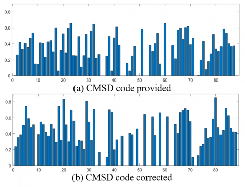
We analyzed the CMSD code provided by the authors, since throughout the analysis, we detected some discrepancies between the algorithm and the proposed model. In general, the discrepancies are centered on the omission or union of values, which caused the values 72 and 88 to be obtained with 0, and the value 78 to be contaminated with equivocally variables. Also, the use of the $\sin$ and $\cos$ function of Matlab in radians and not in degrees; and finally, a discrepancy in the conversion of cylindrical coordinates to cartesian coordinates. An example of the differences between the code provided and the model, is shown in Figure 1, where shows the histograms of image 716 in horse class from Corel-1k, the descriptor provided by the authors is set as “a”, and the corrected one following the model as “b”.
We decided to take the same image that is used as an example in the article where the descriptor is proposed, to find coincidences between the descriptor provided and the data shows in the author's paper. We found that the descriptor provided, which does not faithfully follow the model, delivers the same result shown in the images of their article, likewise, as shown in Figure 1. The feature vector obtained differs with respect to the corrected descriptor, so there is a possibility that the results obtained in their article were made with a version of the descriptor that does not follow the model faithfully. For this reason, we decided to evaluate both versions of the descriptor, to see if the discrepancies affected the performance of the descriptor.
Figure 1. Histograms of the descriptor CMSD
The results of the evaluation using the four metrics, with the Corel-1k, Corel-5k, and Caltech 101 image sets, are shown in Tables 1-3, where the best result is highlighted with “bold”. The evaluation showed that the descriptor correcting the discrepancies between the model and the algorithm, obtained better results on average, so it was decided to use this version of the algorithm, for the subsequent experiments.
Table 1. CMSD evaluation with Corel-1k
|
|
P |
R |
MAP |
ANMRR |
|
Provided |
75.66% |
9.08% |
8.40% |
1.41% |
|
Corrected |
77.33% |
9.28% |
8.64% |
1.31% |
Table 2. CMSD evaluation with Corel-5k
|
|
P |
R |
MAP |
ANMRR |
|
Provided |
32.48% |
3.90% |
2.90% |
4.00% |
|
Corrected |
34.10% |
4.09% |
3.05% |
3.90% |
Table 3. CMSD evaluation with Caltech-101
|
|
P |
R |
MAP |
ANMRR |
|
Provided |
10.16% |
1.56% |
0.99% |
4.58% |
|
Corrected |
10.90% |
1.71% |
1.09% |
4.54% |
With respect to the MIFH descriptor, the literature did not establish the value of $\Delta_{x}$ and $\Delta_{y}$for obtaining the co-occurrence, as well as the type of sub-sampling performed, so an evaluation was performed with different combinations, using average (AVG); minimum (MIN); and maximum (MAX), for sub-sampling, and three combinations of $\Delta_{x}$ and $\Delta_{y}$, which gave a total of nine combinations. For the evaluation, the metrics and image sets Corel-1k (Table 4) and Corel-5k (Table 5) were used, from the evaluation, the combination that was considered the most stable and with the best results was taken, in this case the combination AVG-01.
Table 4. Evaluation of MIFH combinations with Corel-1k
|
|
P |
R |
MAP |
ANMRR |
|
AVG-11 |
73.58% |
8.83% |
7.93% |
1.54% |
|
AVG-10 |
72.58% |
8.71% |
7.95% |
1.59% |
|
AVG-01 |
75.00% |
9.00% |
8.21% |
1.45% |
|
MAX-11 |
73.50% |
8.82% |
8.06% |
1.54% |
|
MAX-10 |
74.33% |
8.92% |
8.15% |
1.49% |
|
MAX-01 |
73.75% |
8.85% |
8.07% |
1.53% |
|
MIN-11 |
74.08% |
8.89% |
7.97% |
1.51% |
|
MIN-10 |
73.58% |
8.83% |
7.94% |
1.54% |
|
MIN-01 |
74.00% |
8.88% |
8.04% |
1.51% |
Table 5. Evaluation of MIFH combinations with Corel-5k
|
|
P |
R |
MAP |
ANMRR |
|
AVG-11 |
28.88% |
3.46% |
2.40% |
4.21% |
|
AVG-10 |
28.72% |
3.44% |
2.40% |
4.22% |
|
AVG-01 |
28.78% |
3.45% |
2.43% |
4.22% |
|
MAX-11 |
27.82% |
3.33% |
2.30% |
4.28% |
|
MAX-10 |
28.43% |
3.40% |
2.35% |
4.24% |
|
MAX-01 |
28.55% |
3.42% |
2.37% |
4.24% |
|
MIN-11 |
28.25% |
3.38% |
2.37% |
4.25% |
|
MIN-10 |
28.22% |
3.38% |
2.34% |
4.25% |
|
MIN-01 |
28.75% |
3.44% |
2.41% |
4.22% |
Figure 2. Images in Caltech-101
Table 6. Results with Corel-1k
|
|
P |
R |
MAP |
ANMRR |
|
CLD |
49.00% |
5.88% |
4.92% |
3.02% |
|
EHD |
56.58% |
6.79% |
5.70% |
2.56% |
|
MSD |
70.75% |
8.49% |
7.58% |
1.70% |
|
CMSD |
77.33% |
9.28% |
8.64% |
1.31% |
|
SED |
61.17% |
7.34% |
6.28% |
2.27% |
|
MIFH |
75.00% |
9.00% |
8.21% |
1.45% |
Table 7. Results with Corel-5k
|
|
P |
R |
MAP |
ANMRR |
|
CLD |
10.22% |
1.23% |
0.64% |
5.37% |
|
EHD |
10.33% |
1.24% |
0.68% |
5.37% |
|
MSD |
26.50% |
3.18% |
2.20% |
4.37% |
|
CMSD |
34.10% |
4.09% |
3.05% |
3.90% |
|
SED |
26.80% |
3.22% |
2.26% |
4.35% |
|
MIFH |
28.78% |
3.45% |
2.43% |
4.22% |
Table 8. Results with Corel-CBIR
|
|
P |
R |
MAP |
ANMRR |
|
CLD |
21.38% |
2.29% |
1.76% |
1.84% |
|
EHD |
23.41% |
2.45% |
1.83% |
1.79% |
|
MSD |
25.68% |
2.76% |
2.01% |
1.73% |
|
CMSD |
37.27% |
3.99% |
3.27% |
1.45% |
|
SED |
23.14% |
2.47% |
1.70% |
1.79% |
|
MIFH |
32.04% |
3.45% |
2.66% |
1.57% |
Table 9. Results with Caltech-101
|
|
P |
R |
MAP |
ANMRR |
|
CLD |
14.26% |
2.18% |
1.59% |
4.43% |
|
EHD |
20.43% |
3.57% |
2.63% |
4.10% |
|
MSD |
8.87% |
1.35% |
0.87% |
4.63% |
|
CMSD |
10.90% |
1.71% |
1.09% |
4.54% |
|
SED |
7.50% |
1.17% |
0.69% |
4.67% |
|
MIFH |
10.51% |
1.58% |
1.03% |
4.57% |
Figure 3. Images in Corel-5k
The evaluation was carried out with the rest of the descriptors, with the adjustments recommended by the authors. The results are shown in Table 6-9. Where we observed that the CMSD and MIFH descriptors delivered better results in the Corel-1k, Corel-5k and Corel-CBIR datasets. However, in the Caltech-101 dataset, which has object categories, and some of the classes contain non-real images, i.e., drawings or cartoons, as shown in Figure 2. The descriptors of the MPEG-7 standard stood out, with EHD being the best evaluated. This could be since the descriptors proposed by the standard are oriented to retrievals in terms of shape, color, and textures, which are better defined in Caltech-101.
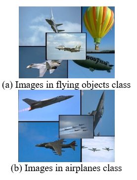
Apparently, retrieval with concept classes improves using descriptors that use more than one low-level feature, however, when retrieval is performed on images with object classes and with illustrations, descriptors representing one low-level feature performed better. Despite this, it would remain to analyze and test the results, using more sets of images, with object classes. In general, the most complicated classes for most of the descriptors are those referring to a specific place, since they contained a great diversity of contents with no apparent visual relationship, as well as classes with contents like another, as shown in Figure 3 which presents examples of images in the class airplanes and the class flying objects of Corel-5k.
2.3 Weakness detection
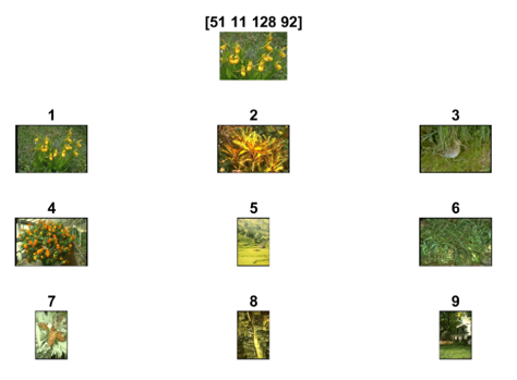
In the evaluation, we detected some problematic images and classes, some of the retrievals presented errors apparently unrelated to the query image such as images 1, 6, and 8 shown in Figure 4. Weakness detection focused on the best performing descriptors in the evaluation, in this case the descriptors CMSD and MIFH. To detect areas within the images that could affect the retrieval. We coded a system to select and cut parts of a query image, looking for a relationship between an area or part of the image and the erroneous images, trying to detect the reason for confusion and weaknesses in the descriptors. Figure 5 shows a retrieval performed with the system, where the recovered images are shown with a slice of the query image of Figure 4, placing as name the coordinates of crop.
Figure 4. Flower retrieval with CMSD
We detected in some retrieves that the confusion could be due to the information introduced by areas in the background. because in the queries performed with a crop of the background area, the unwanted images were retrieved in a better position, even in some situations, the retrieve got others similar unwanted images. However, in some cases we did not find a relationship between a specific area of the image and the unwanted image, so the confusion was not due to a specific area.
Figure 5. Retrieval using crop of flowers image
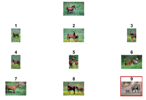
We found that the images could have a relationship in the direction or proportion of textures and color, despite not being distributed in the same way. i.e., Figure 6 despite not having an apparent visual relationship, have a similar perspective, and contain similar colors, when quantified, and despite having different textures, they maintain some proportions, in relation to texture-color. Likewise, it was observed that queries on saturated images or with a low variety of colors, i.e., with a poorly distributed color histogram, retrieved saturated images, even though they were not the same colors, as the case shown in Figure 7.
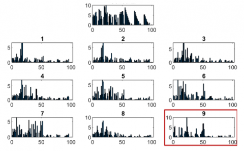
Looking for the possible weaknesses responsible for the unwanted image retrieved, an attempt was made to induce undesired retrievals by selecting images that had characteristics that could be cause an erroneous retrieval. An analysis of the images considered as problematic was performed, obtaining their difference histograms, as shown in Figure 8, for each of the values in the feature vector, with the intention of obtaining values within the vector that caused the confusion, or values that could be used to avoid it.
Figure 6. Beach retrieval with CMSD
Figure 7. Horse retrieval with MIFH
Figure 8. Histogram differences of horse query with MIFH
In the experiment we found that the values that caused confusion were often the values with zero in the color histogram. In the case of the CMSD the saturated images looked similarity in the color histogram since the only thing that differentiated them from the 72 color values were 6 to 10 values having a total of 62 to 66 values the same since there were no colors in that range. In the case of the MIFH descriptor, despite not having more than 54 color values, presented a similarly case, since by generalizing the color more, the colors that apparently was different, the quantification considered the same value.
To find the most or least discriminant values, we chose to calculate the dispersion measures of the feature vector. We used the Range Eq. (13), the standard deviation Eq. (14) and the coefficient of variation Eq. (15). Where X is the population; x each of its elements; N, the amount of data; and $\mu$ the average. With the dispersion measures we looked for values with wide ranges, a small standard deviation between class images and large between classes, and with a coefficient of variation greater than 26%. This was to detect the most discriminating values and conversely to detect values that were not very discriminating.
Range $=\max (X)-\min (X)$ (13)
$\sigma=\sqrt{\frac{\sum(x-\mu)^{2}}{N}}$ (14)
$C V=\frac{\sigma}{\mu}$ (15)
During the evaluation we found that the descriptor values in general did not behave in an equivalent way, varying their discrimination in each class, and apart from the null values, no specific value was detected that did not discriminate or discriminated more than the others. In the case of the MIFH descriptor, it was found that the values where the edges of the image were represented, from value 55 to 102, had values that were apparently not very discriminating and could even be causing confusion. In general, the last five values of each of the edge feature integration, i.e., the values [66, 67,…,70, 81, 82,…, 86, 98, 99,…, 102]. Since the majority images obtained a zero, and in some other cases only the values [1.3863, 1.0986, 0.69315], and with no apparent relationship between classes.
2.4 Discussion
Some of the errors are due to problems in the image sets, since there are classes that are very similar, or that have very varied contents, as is the case of the classes that belong to a specific region, for example, the Roma class. Likewise, there are images that could well belong to more than one class, or that have more information of another class than the one in which they are labeled. It appears that using more than one low-level feature of the image decreases its effectiveness in lower-level retrieval queries. In general, MIFH and CMSD can be considered as the best performing descriptors, however, they seem to be sensitive to the background of the images, as it introduces information that affects retrieval, more so in cases where the background is present in a higher percentage than the object of interest. As well as in cases where the background is present in a higher percentage than the object of interest. The descriptors also give great importance to color, in the CMSD descriptor 82% of the vector belongs to color, and in the case of MIFH, despite being less than 53%, the color histogram is directly obtained from the HSV color space, it means, depend entirely on the color of the image, not on a relation, unlike CMSD. On the other hand, the generalization of color by quantization causes that, apparently different colors are cataloged as the same, since from $2^{24}$ they become 72 and 54 colors, respectively. In addition, some values in the feature vectors of the descriptors seem to be unrepresentative, which could be causing erroneous retrievals.
To analyze ways to remedy some of the weaknesses found, experiments are presented with a series of adjustments and changes in the MIFH and CMSD descriptors, considering their best version, being these the ones that on average obtained the best results in the evaluation. The experiments will be performed using the four sets of images and the four metrics, following the same specifications as stated in Section 2 and using the same query images. The first part details the settings, modifications and results obtained with the MIFH descriptor, followed by the variants and results obtained with the CMSD descriptor.
3.1 MIFH descriptor
The MIFH descriptor presented some apparently unrepresentative values in its feature vector, some of them were null and we did not find apparent relationship between images and values. Therefore, two adjustments were made to try to avoid the possible confusion induced by these values.
Likewise, having a wide range when performing the edge integration, the quantification in MIFH could cause loss of relevant information, so two modifications were made trying not to lose relevant information.
During the evaluation, it was detected that the background color of the image caused a retrieval of images belonging to another class with similar background colors. To prevent the background color from affecting the retrieval, a modification was performed.
We decided to combine variants to try to improve the retrieval. MIFH-V6, is the combination of MIFH-V1 with MIFH-V3, MIFH-V6 use the same quantified method of MIFH-V3 but removes the last five values of each edge integration. The combination of MIFH-V1 and MIFH-V5 is MIFH-V7, this combination gives weights to the colors, and removes the last five values of each edge integration. MIFH-V8, use the same quantified method of MIFH-V3 and gives weights to the colors like MIFH-V5. Finally, MIFH-V9 is the combination of MIFH-V6 and MIFH-V5, using the same quantified method of MIFH-V3, but gives weights to the color, and removes the last five values of each edge integration. The results obtained with the proposed variants are shown in Table 10-13, with the results that exceed the original descriptor in “bold”.
Table 10. MIFH adjustments with Corel-1k
|
|
P |
R |
MAP |
ANMRR |
|
MIFH-V1 |
75.67% |
9.08% |
8.35% |
1.41% |
|
MIFH-V2 |
75.42% |
9.05% |
8.34% |
1.43% |
|
MIFH-V3 |
75.33% |
9.04% |
8.21% |
1.44% |
|
MIFH-V4 |
74.17% |
8.90% |
8.21% |
1.50% |
|
MIFH-V5 |
74.58% |
8.95% |
8.25% |
1.47% |
|
MIFH-V6 |
74.92% |
8.99% |
8.19% |
1.46% |
|
MIFH-V7 |
74.92% |
8.99% |
8.29% |
1.46% |
|
MIFH-V8 |
74.42% |
8.93% |
8.12% |
1.49% |
|
MIFH-V9 |
74.92% |
8.99% |
8.21% |
1.46% |
Table 11. MIFH adjustments with Corel-5k
|
|
P |
R |
MAP |
ANMRR |
|
MIFH-V1 |
28.92% |
3.47% |
2.44% |
4.22% |
|
MIFH-V2 |
28.82% |
3.46% |
2.44% |
4.22% |
|
MIFH-V3 |
29.27% |
3.51% |
2.46% |
4.20% |
|
MIFH-V4 |
28.77% |
3.45% |
2.43% |
4.22% |
|
MIFH-V5 |
29.27% |
3.51% |
2.48% |
4.19% |
|
MIFH-V6 |
29.47% |
3.54% |
2.48% |
4.18% |
|
MIFH-V7 |
29.17% |
3.50% |
2.48% |
4.20% |
|
MIFH-V8 |
29.42% |
3.53% |
2.48% |
4.19% |
|
MIFH-V9 |
29.68% |
3.56% |
2.50% |
4.17% |
Table 12. MIFH adjustments with Corel-CBIR
|
|
P |
R |
MAP |
ANMRR |
|
MIFH-V1 |
31.96% |
3.44% |
2.67% |
1.57% |
|
MIFH-V2 |
31.97% |
3.44% |
2.65% |
1.57% |
|
MIFH-V3 |
31.56% |
3.39% |
2.60% |
1.58% |
|
MIFH-V4 |
31.32% |
3.38% |
2.60% |
1.58% |
|
MIFH-V5 |
31.92% |
3.42% |
2.65% |
1.57% |
|
MIFH-V6 |
31.58% |
3.39% |
2.59% |
1.58% |
|
MIFH-V7 |
31.94% |
3.43% |
2.65% |
1.57% |
|
MIFH-V8 |
31.02% |
3.32% |
2.54% |
1.60% |
|
MIFH-V9 |
31.18% |
3.34% |
2.55% |
1.59% |
Table 13. MIFH adjustments with Caltech-101
|
|
P |
R |
MAP |
ANMRR |
|
MIFH-V1 |
10.46% |
1.57% |
1.03% |
4.57% |
|
MIFH-V2 |
10.42% |
1.56% |
1.03% |
4.57% |
|
MIFH-V3 |
10.60% |
1.61% |
1.05% |
4.56% |
|
MIFH-V4 |
10.46% |
1.59% |
1.03% |
4.57% |
|
MIFH-V5 |
10.46% |
1.58% |
1.04% |
4.57% |
|
MIFH-V6 |
10.52% |
1.59% |
1.03% |
4.57% |
|
MIFH-V7 |
10.51% |
1.58% |
1.04% |
4.57% |
|
MIFH-V8 |
10.56% |
1.62% |
1.07% |
4.56% |
|
MIFH-V9 |
10.56% |
1.61% |
1.05% |
4.56% |
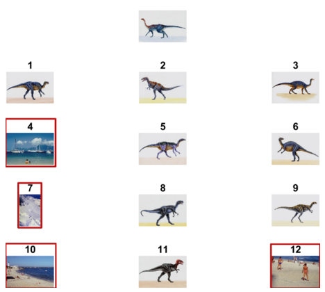
We observed that the variants improve in some metrics and in certain sets, however, it is not possible to obtain a stable variant that surpasses the original descriptor, which is possibly because some of the variants, despite strengthening a weakness, increased or generated a new weakness. An example is shown in Figures 9-10, where retrieval with MIFH and MIFH-V5 is presented, in a class where the MIFH descriptor performs very well since most of the images have the same white background, which affects the MIFH-V5 variant, since, by not considering the background relevant, it retrieves in better position unwanted images, which have a similar color to the object of interest.
The result shows that MIFH-V3 was the most stable variant in average, since it obtains better results than the original MIFH in three of the four image datasets, however, it would be necessary to experiment with different quantification bins to improve the results even in the Corel-CBIR image set. In this way it could be considered a possible option to improve the performance of the descriptor.
Figure 9. Dinosaur retrieval with MIFH
Figure 10. Dinosaur retrieval with MIFH-V5
3.2 CMSD descriptor
The CMSD descriptor gave the best results in the evaluation. However, it is limited to small structures, so it was decided to integrate more sizes of structures, scaling the input image in a pyramidal way, thus obtaining in the smaller images larger structures present in the image. Following this idea, three variants are presented:
Likewise, we made an adjustment to the similarity measure used, calculating the sum of the distances Manhattan Eq. (16), for each feature vector by dividing them by the size of the vector length, as shown in Eq. (17), to avoid that a feature has a higher relevance.
$D(s, q)=\sum_{i=1}^{N_{f}}\left|s_{i}-q_{i}\right|$ (16)
$M 3(s, q)=\sum_{c=1}^{C} \frac{\sum_{i=1}^{N_{f}^{c}}\left|s_{i}^{c}-q_{i}^{c}\right|}{N_{f}^{c}}$ (17)
where, s is set as the vector of an image, q the vector of the query image, Nfthe length of the feature vector, $S^{C}$ and qc the vector of each of its C features, and $N_{f}^{c}$ its length. In the case of CMSD it is set as C=3, since it considers edge, color, and intensity. The results are shown in Tables 14-17, where CMSD-V4; CMSD-V5; and CMSD-V6, refers to the results using the CMSD-V1; CMSD-V2; and CMSD-V3 with the modified Manhattan distance measure respectively.
Table 14. CMSD adjustments with Corel-1k
|
|
P |
R |
MAP |
ANMRR |
|
CMSD-V1 |
77.08% |
9.25% |
8.68% |
1.33% |
|
CMSD-V2 |
76.08% |
9.13% |
8.49% |
1.39% |
|
CMSD-V3 |
79.08% |
9.49% |
8.91% |
1.21% |
|
CMSD-V4 |
76.83% |
9.22% |
8.47% |
1.35% |
|
CMSD-V5 |
75.25% |
9.03% |
8.25% |
1.44% |
|
CMSD-V6 |
76.42% |
9.17% |
8.52% |
1.37% |
We observed that the variants in general fail to outperform the original. However, it is improved in the Caltech-101 dataset, so apparently the use of different size structures could help, to improve the retrieval at level two, which refers to objects. CMSD-V3 was the most stable variant, since it obtained better results on three of the four image datasets than the original. So apparently the reduction of color detail can benefit in the detection of larger structures, only in the one by one reduction in the quantization bins of the H channel in HSV color space.
Table 15. CMSD adjustments with Corel-5k
|
|
P |
R |
MAP |
ANMRR |
|
CMSD-V1 |
30.95% |
3.71% |
2.72% |
4.09% |
|
CMSD-V2 |
29.97% |
3.60% |
2.60% |
4.15% |
|
CMSD-V3 |
32.22% |
3.87% |
2.89% |
4.02% |
|
CMSD-V4 |
25.37% |
3.04% |
2.12% |
4.43% |
|
CMSD-V5 |
23.17% |
2.78% |
1.83% |
4.56% |
|
CMSD-V6 |
26.97% |
3.24% |
2.28% |
4.33% |
Table 16. CMSD adjustments with Corel-CBIR
|
|
P |
R |
MAP |
ANMRR |
|
CMSD-V1 |
37.04% |
3.99% |
3.23% |
1.45% |
|
CMSD-V2 |
34.67% |
3.73% |
2.96% |
1.50% |
|
CMSD-V3 |
37.34% |
4.02% |
3.27% |
1.44% |
|
CMSD-V4 |
36.03% |
3.85% |
3.09% |
1.48% |
|
CMSD-V5 |
30.75% |
3.27% |
2.50% |
1.61% |
|
CMSD-V6 |
37.18% |
3.97% |
3.23% |
1.45% |
Table 17. CMSD adjustments with Caltech-101
|
|
P |
R |
MAP |
ANMRR |
|
CMSD-V1 |
11.36% |
1.85% |
1.21% |
4.51% |
|
CMSD-V2 |
10.90% |
1.76% |
1.15% |
4.53% |
|
CMSD-V3 |
11.64% |
1.87% |
1.23% |
4.50% |
|
CMSD-V4 |
13.57% |
2.25% |
1.55% |
4.41% |
|
CMSD-V5 |
12.44% |
2.00% |
1.37% |
4.47% |
|
CMSD-V6 |
13.64% |
2.25% |
1.55% |
4.41% |
The combined use of texture and color to describe images seems to improve the representation of images retrievals in conceptual classes, however, it does not seem to improve in object classes. In average, the descriptors CMSD and MIFH show better results than the rest. In spite of this, we can mentioned three possible weaknesses, related to unwanted images in the retrieval, or without an apparent relation to the query image: one of them is color, both its representation and its importance; sensitivity to background information; and finally, some weaknesses in the representation, since there are values within their vectors that are not very representative and despite the fact that the descriptors analyzed consider the relationship between two image features, unwanted images are still obtained very similar to those of a low-level descriptor, since they tend to give greater importance to a feature.
In the experiments, some variants perform better than the original descriptors, especially in level 2 retrievals. However, it would be necessary to study in which type of images they work better than the current ones, since they are still not stable enough to maintain the best result in all the sets, so their use would be recommended in specific cases. In addition, it is necessary to study and evaluate the variants with other combinations and adjustments, such as changing the quantification method. The modifying descriptors to address a weakness may affect their performance by generating new weaknesses, so it is not an easy task. Therefore, the area required research and information, since they could not only benefit image retrieval systems, but also any other system that requires image analysis. Since most systems currently use descriptors that represent a low-level feature and do not consider the relationships between them, losing relevant information that is not found directly in the image, information that could facilitate its analysis or relate more directly to high-level features.
The authors would like to thank the Tecnológico Nacional de México, the Centro Nacional de Investigación y Desarrollo Tecnológico (CENIDET) and the authors who provided their descriptor codes and information about them. K. Salvador Aguilar-Domínguez thanks the Consejo Nacional de Ciencia y Tecnología (CONACYT) under the concept of doctoral scholarship.
[1] Ahmad, J., Sajjad, M., Rho, S., Baik, S.W. (2016). Multi-scale local structure patterns histogram for describing visual contents in social image retrieval systems. Multimedia Tools and Applications, 75(20): 12669-12692. https://doi.org/10.1007/s11042-016-3436-9
[2] RajaSenbagam, T., Shanmugalakshmi, R. (2017). A survey on content based image retrieval for reducing semantic gap. International Research Journal of Engineering and Technology (IRJET), 4(12).
[3] Kishore, D., Rao, C.S. (2020). A multi-class SVM based content based image retrieval system using hybrid optimization techniques. Traitement du Signal, 37(2): 217-226. https://doi.org/10.18280/TS.370207
[4] Hamreras, S., Benıtez-Rochel, R., Boucheham, B., Molina-Cabello, M.A., Lopez-Rubio, E. (2019). Content based image retrieval by convolutional neural networks. International Work-Conference on the Interplay Between Natural and Artificial Computation, 2: 277-286. https://doi.org/10.1007/978-3-030-19651-6
[5] Chavda, S.M., Mahesh, G.M. (2019). Content-based image retrieval: The state of the. International Journal of Next-Generation Computing, 10(3).
[6] Zin, N.A.M., Yusof, R., Lashari, S.A., Mustapha, A., Senan, N., Ibrahim, R. (2018). Content-based image retrieval in medical domain: A review. Journal of Physics: Conference Series, 1019(12). https://doi.org/10.1088/1742-6596/1019/1/012044
[7] Li, X., Yang, J., Ma, J. (2021). Recent developments of content-based image retrieval (CBIR). Neurocomputing, 452: 675-689. https://doi.org/10.1016/J.NEUCOM.2020.07.139
[8] Tyagi, V. (2017). Content- Based Image Retrieval (Ideas, Influences, and Current Trends). Springer, Singapore.
[9] Chen, Y., Wang, J.Z., Krovetz, R. (2003). An unsupervised learning approach to content-based image retrieval. IEEE Proceedings of the International Symposium on Signal Processing and Its Applications, pp. 197-200. https://doi.org/10.1109/ISSPA.2003.1224674
[10] Smeulders, M.W., Worring, M., Santini, S., Gupta, A., Jain, R. (2000). Content-based image retrieval at the end of the early years. IEEE Transactions on Pattern Analysis and Machine Intelligence, 22(12): 1349-1380. https://doi.org/10.1109/34.895972
[11] Tsuhan, C. (2005). From low-level features to high-level semantics: Are we bridging the gap? Proceedings - Seventh IEEE International Symposium on Multimedia, ISM 2005, 2005: 179. https://doi.org/10.1109/ISM.2005.62
[12] Deldjoo, Y., Elahi, M., Quadrana, M., Cremonesi, P. (2018). Using visual features based on MPEG-7 and deep learning for movie recommendation. International Journal of Multimedia Information Retrieval, 7(4): 207-19. https://doi.org/10.1007/s13735-018-0155-1
[13] Liu, J., Wang, Z., Liu, H. (2019). HDS-SP: A novel descriptor for skeleton-based human action recognition. Neurocomputing, 385: 22-32. https://doi.org/10.1016/j.neucom.2019.11.048
[14] Wang, S., Han, K., Jin, J. (2019). Review of image low-level feature extraction methods for content-based image retrieval. Sensor Review, 39(6): 783-809. https://doi.org/10.1108/SR-04-2019-0092
[15] Nazir, A., Ashraf, R., Hamdani, T., Ali, N. (2018). Content based image retrieval system by using HSV color histogram, discrete wavelet transform and edge histogram descriptor. 2018 International Conference on Computing, Mathematics and Engineering Technologies: Invent, Innovate and Integrate for Socioeconomic Development, ICoMET 2018 - Proceedings, 2018-Janua, pp. 1-6. https://doi.org/10.1109/ICOMET.2018.8346343
[16] Alzu’bi, A., Amira, A., Ramzan, N. (2017). Content-based image retrieval with compact deep convolutional features. Neurocomputing, 249: 95-105. https://doi.org/10.1016/j.neucom.2017.03.072
[17] Wei, S., Liao, L., Li, J., Zheng, Q., Yang, F., Zhao, Y. (2019). Saliency inside: Learning attentive CNNs for content-based image retrieval. IEEE Transactions on Image Processing, 28(9): 4580-4593. https://doi.org/10.1109/TIP.2019.2913513
[18] Kishore, D., Rao, C.S. (2021). Content-based image retrieval system based on fusion of wavelet transform, texture and shape features. Mathematical Modelling of Engineering Problems, 8(1): 110-116. https://doi.org/10.18280/MMEP.080114
[19] Srivastava, P., Khare, M., Khare, A. (2020). Combining local binary pattern and speeded-up robust feature for content-based image retrieval. 12th Asian Conference, ACIIDS 2020 Phuket, pp. 366-376.
[20] Raza, A., Nawaz, T., Dawood, H., Dawood, H. (2019). Square texton histogram features for image retrieval. Multimedia Tools and Applications, 78(3): 2719-2746. https://doi.org/10.1007/s11042-018-5795-x
[21] Khaldi, B., Aiadi, O., Lamine, K.M. (2020). Image representation using complete multi-texton histogram. Multimedia Tools and Applications, 79(11-12): 8267-8285. https://doi.org/10.1007/s11042-019-08350-1
[22] Raza, A., Dawood, H., Dawood, H., Shabbir, S., Mehboob, R., Banjar, A. (2018). Correlated primary visual texton histogram features for content base image retrieval. IEEE Access, 6: 46595-46616. https://doi.org/10.1109/ACCESS.2018.2866091
[23] Manjunath, B.S., Salembier, P., Sikora, T. (2002). Introduction to MPEG-7. Multimedia Content Description Interface.
[24] Julesz, B. (1981). Textons, the elements of texture perception, and their interactions. Nature, 290(5802).
[25] Liu, G.H., Li, Z.Y., Zhang, L., Xu, Y. (2011). Image retrieval based on micro-structure descriptor. Pattern Recognition, 44(9): 2123-2133. https://doi.org/10.1016/j.patcog.2011.02.003
[26] Dawood, H., Alkinani, M.H., Raza, A., Dawood, H., Mehboob, R., Shabbir, S. (2019). Correlated microstructure descriptor for image retrieval. IEEE Access, 7: 55206-55228. https://doi.org/10.1109/ACCESS.2019.2911954
[27] Wang, X., Wang, Z. (2013). A novel method for image retrieval based on structure elements’ descriptor. Journal of Visual Communication and Image Representation, 24(1): 63-74. https://doi.org/10.1016/j.jvcir.2012.10.003
[28] Chu, K., Liu, G.H. (2020). Image retrieval based on a multi-integration features model. Mathematical Problems in Engineering. https://doi.org/10.1155/2020/1461459
[29] Eakins, J., Graham, M. (1999). Content-based image retrieval. Technical Report, University of Northumbria at Newcastle.
[30] Wang, J.Z., Li, J., Wiederhold, G. (2001). SIMPLIcity: Semantics-sensitive integrated matching for picture libraries. IEEE Transactions on Pattern Analysis and Machine Intelligence, 23(9): 947-963.
[31] Li, J.W.J.Z. (2008). Real-time computerized annotation of pictures. IEEE Transactions on Pattern Analysis and Machine Intelligence, 30(6): 985-1002.
[32] Bian, W.T.D. (2010). Biased discriminant Euclidean embedding for content-based image retrieval. IEEE Transactions on Image Processing, 19(2): 545-54.
[33] Li, F.F., Fergus, R., Perona, P. (2004). Learning generative visual models from few training examples: An incremental Bayesian approach tested on 101 object categories. In 2004 Conference on Computer Vision and Pattern Recognition Workshop, pp. 178-178. https://doi.org/10.1109/CVPR.2004.383
[34] Lux, M., Marques, O. (2013). Visual information retrieval using Java and lire. Synthesis Lectures on Information Concepts, Retrieval, and Services, 5(1): 1-112. https://doi.org/10.2200/S00468ED1V01Y201301ICR025