Yin Chen
© 2021 IIETA. This article is published by IIETA and is licensed under the CC BY 4.0 license (http://creativecommons.org/licenses/by/4.0/).
OPEN ACCESS
MRI image analysis of brain regions based on deep learning can effectively reduce the workload of doctors in reading films and improve the accuracy of diagnosis. Therefore, deep learning models have great application prospects in the classification and prediction of Alzheimer’s patients and normal people. However, the existing research has ignored the correlation between small abnormalities in local brain regions and changes in brain tissues. To this end, this paper studies an Alzheimer’s disease identification and classification model based on the convolutional neural network (CNN) with attention mechanisms. In this paper, the attention mechanisms were introduced from the regional level and the feature level, and the information of brain MRI images was fused from multiple levels to find out the correlation between the slices in brain MRI images. Then, a spatio-temporal graph CNN with dual attention mechanisms was constructed, which made the network model more attentive to the salient channel features while eliminating the impact of certain noise features. The experimental results verified the effectiveness of the constructed model in identification and classification of Alzheimer’s disease.
Alzheimer’s disease, identification and classification, attention mechanism, convolutional neural network
Alzheimer’s disease is an incurable degenerative disease of the nervous system with insidious onset and chronic progression, mainly manifested in memory impairment, cognitive impairment, visual impairment and executive dysfunction, etc. [1-6]. Fortunately, with the continuous development of the magnetic resonance imaging (MRI) technology, MRI images have become a necessary tool for observation of brain activities and diagnosis of brain diseases [7-10]. However, due to the high efficiency of the MRI technology, the large number of MRI images generated has led to an increase in the workload of doctors in film reading, and what is more, manual film reading largely depends on doctors’ work experience, which may lead to misdiagnoses [11-14]. Therefore, analysis of brain MRI images based on the deep learning technology has become a good choice. Applying a deep learning model in the analysis of MRI images to classify and predict Alzheimer’s patients and normal people is helpful to the development of an intelligent auxiliary diagnosis system for Alzheimer’s disease, and realize accurate identification of the high-risk groups of this disease, and in this way, subsequent treatment can be well prepared [15-17].
Fu’adah et al. [18] proposed using the convolutional neural network of the AlexNet architecture as a method to develop an automatic classification system for Alzheimer’s disease. The experiment achieved classification of non-dementia, very mild dementia, mild dementia and moderate dementia from 664 MRI datasets. Guan et al. [19] discussed the influences of different network architectures on the transferability of the model, found that appropriate deepening or widening of the network can increase transferability, analyzed the contributions of different parts of the 3D CNN to transferability, and verified that fine-tuning the CNN can significantly improve transferability. Villain et al. [20] proposed a new visualization technology to describe the decision-making of CNN in classification tasks, with the brain MRI images as the input to the traditional 3D CNN. The model can correct the brain images by linearly increasing the feature intensity of the corresponding regions, which is suitable for regions of different sizes, positions, and in closed brain tissues that contain different types of features. Folego et al. [21] customized and trained the convolutional neural network for brain MRIs based on the data sets available in online databases. The proposed method ADNet was evaluated in Alzheimer’s disease identification and proved superior to the several existing methods. Yildirim et al. [22] proposed a hybrid method. According to the architecture used, the disease progression was divided into 4 stages. The hybrid model was proposed based on the Resnet50 method. The results were obtained by Alexnet, Resnet50, Densenet201, Vgg16 and the hybrid method, respectively, and the hybrid model proposed reached an accuracy of 90%. Salehi et al. [23] used the convolutional neural network for early diagnosis and classification of MRI images of Alzheimer’s disease. It used 3 types of ADNI images, with totally 1512 cases of mild Alzheimer’s disease, 2633 cases of normal and 2480 cases of Alzheimer’s disease. Compared with many other models, this model achieved an accuracy of 99%, showing good performance.
However, the existing research has some problems in the auxiliary diagnosis of Alzheimer’s disease - it has ignored small abnormalities in local brain regions, or used voxel-based methods generating high feature dimensions, which makes classification time-consuming and prone to over-fitting. The changes of brain tissues over time actually have certain correlations, and failure to fuse regional features will greatly affect the accuracy of disease identification. Therefore, how to extract and learn the features of MRI images and further perform accurate classification is still the focus of the current research work. This paper studies the Alzheimer’s disease identification and classification model based on the CNN with attention mechanisms. Section 2 introduces in detail the operation steps involved in the deep CNN used. Section 3 introduces attention mechanisms from the regional level and the feature level, realize the fusion of brain MRI image information from multiple levels, and finds the correlations between the slices in the brain MRI images. Section 4 improves the deep CNN and constructs the spatio-temporal graph CNN with dual attention mechanisms, so that the network model pays more attention to the salient channel features and eliminates the impact of certain noise features. The experimental results prove the effectiveness of the proposed model in the identification and classification of Alzheimer’s disease.
The operations involved in the deep CNN mainly include 7 aspects, namely convolution, batch processing, activation function processing, pooling, fully connected layer processing, separable convolution processing and receptive field.
Specifically, convolution is to slide the convolution kernel over the input brain MRI images, that is, to perform point-wise multiplication and summation of the elements on the convolution kernel and the pixels on the corresponding input brain MRI image.
Batch processing is approximately equivalent to the normalization of images, that is, the operation of normalizing the pixel values of a small batch of pixels in the input brain MRI images to a certain range to avoid large numerical oscillations during network training. Suppose that the pixel values of the input pixels with a batch size of n is denoted as A=(a1,...,ai,...,an). Batch processing may damage the features that the neural network has learned through network training. In order to mitigate this problem, the learnable parameters set are represented by δ and α.
Assuming that the parameter set to avoid the denominator being zero is represented by υ, that the mean value by λa, that the variance by ε2, that the normalized output by ȃi, and that the output after batch processing by pi, the calculation process of batch processing is given in Eq. (1)-(4):
$\lambda_{A}=\frac{1}{n} \sum_{i=1}^{n} a_{i}$ (1)
$\varepsilon^{2}=\frac{1}{n} \sum_{i=1}^{n}\left(\lambda_{A}-a_{i}\right)^{2}$ (2)
$\hat{a}_{i}=\frac{a_{i}-\lambda_{A}}{\sqrt{\varepsilon^{2}+v}}$ (3)
$p_{i}=\delta \hat{a}_{i}+\alpha$ (4)
The nonlinear activation functions commonly used in deep CNNs include the Sigmoid function and the ReLU function, expressed as Eq. (5) and (6):
$S I G(a)=\frac{1}{1+e^{-a}}$ (5)
$\operatorname{RELU}(a)=\max (0, a)$ (6)
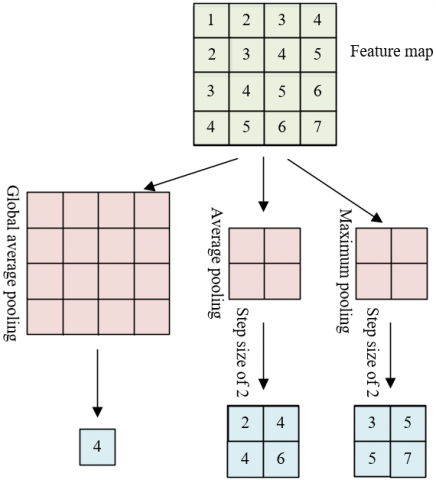
The pooling operations of deep CNNs include maximum pooling, average pooling, and global average pooling, as shown in Figure 1. The fully connected layer is composed of multiple neurons with multiple inputs. All the inputs are weighted and then added to the bias term. After the processing by the activation function, the network output can be obtained.
Figure 1. Different forms of pooling operations
Suppose that the m-dimensional input values of the neurons in the fully connected layer are denoted as a1,...,ai,...,am, that the connection weight of each input value to the j-th neuron as θ1j,...,θij,...,θmj, that the bias term of the j-th neuron as rj, that the activation function as Φ, that the output value of the j-th neuron as bj, the calculation process of the fully connected layer is given in Eq. (7):
$b_{j}=\Phi\left(\sum_{i=1}^{m} a_{i} * \theta_{i j}+r_{j}\right)$ (7)
In order to improve the nonlinear fitting ability of the network and enable it to complete the complex logic task of Alzheimer’s disease identification and classification, it is necessary to build a deep CNN model with multiple hidden layers. A multi-layer perceptron where each neuron in the upper layer is connected to all the neurons in the lower layer can be regarded as a form of full connection. Suppose that in the first network layer of a multilayer perceptron with a hidden layer and an output layer, the bias term of the first neuron is denoted as r11, where the superscript and the subscript indicate the network layer No. and the neuron No., respectively. Suppose that the connection weight of the i-th neuron in the k-th layer and the j-th neuron in the k+1-th layer is denoted as θτij, and that the output of the j-th neuron in the i-th layer is denoted as pij. The calculation process of b1 and b2 is shown in Eq. (8), (9) and (10):
$p_{j}^{1}=\Phi\left(r_{j}^{1}+\sum_{i=1}^{3} a_{i} * \theta_{i j}^{1}\right)$ (8)
$b_{1}=\Phi\left(r_{j}^{2}+\sum_{i=1}^{2} p_{j}^{1} * \theta_{j 1}^{2}\right)$ (9)
$b_{2}=\Phi\left(r_{2}^{2}+\sum_{i=1}^{2} p_{j}^{1} * \theta_{j 2}^{2}\right)$ (10)
In order to effectively reduce the number of parameters in the constructed deep CNN and increase the computation rate of Alzheimer’s disease identification and classification, this paper proposed setting the deep separable convolutional layer. The deep separable convolution takes two steps - spatial relationship learning and inter-channel relationship learning. In the first step, the last dimension of the convolution kernel is 1, and in the second step, channel information is fused based on the 1×1 convolution.
To obtain better Alzheimer’s disease identification and classification results, the network needs to extract more complete image feature information, that is, it needs to have a larger network receptive field. In fact, the size of the receptive field of the convolutional layer, which is the basic layer of the network, is determined together by the size of the convolution kernel and the brain MRI image feature map of the previous layer. As the resolution of the feature map decreases, the receptive field of the network will enlarge, and the reduction of the feature map resolution can be achieved through setting of multiple downsampling layers in the network.
The loss functions involved in the network training of the constructed deep CNN mainly include the least absolute deviation, the least square error and the cross entropy error, denoted as LSD, LSE and CEE, respectively. Specifically, the LSD loss function is to minimize the sum of the absolute values of the differences between the predicted classification results and the real situation. Suppose that the i-th predicted classification result is denoted as YCi, and that the i-th real situation as ZSi. The calculation formula is shown in Eq. (11):
$L S D=\sum_{i=1}^{m}\left|Y C_{i}-Z S_{i}\right|$ (11)
The LSE loss function is to minimize the sum of squares of the differences between the predicted classification results and the real situation. The calculation formula is shown in Eq. (12):
$L S E=\sum_{i=1}^{m}\left(Y C_{i}-Z S_{i}\right)^{2}$ (12)
The CEE loss function can be used to characterize the distance between two probability distributions. The smaller the CEE, the smaller the difference between the two probability distributions. The calculation formula is shown in Eq. (13):
$C E E=-\sum Z S(a) \log (Y C(a))$ (13)
In order to minimize the values of the loss functions, the gradient descent algorithm was adopted as the optimization algorithm. Assuming that the deep neural network model is denoted as DN(ω), that the derivative of the j-th variable ωj of the model can be derived according to the chain rule, and that the learning rate that controls the size of the parameters in each update is denoted as β. The calculation formula is shown in Eq. (14):
$\omega_{j}:=\omega_{j}-\beta \frac{\partial}{\partial \omega_{j}} D N(\omega)$ (14)
For the Alzheimer’s disease identification and classification task based on brain MRI images, since the feature map and the input image need to be consistent dimensionally, the CNN constructed in the previous section was used as the basic skeleton for model design. In the slice sequence of brain MRI images, adjacent slices with higher similarity have more similar information. In order to realize the fusion of brain MRI image information from multiple levels, the attention mechanisms were introduced from two levels - the regional level and the feature level, with a view to finding the correlations between the slices in the brain MRI images.
Figure 2. Design of the attention mechanism at the regional level
Figure 2 shows the design principle of the attention mechanism at the regional level. Regarding this level, pooling, which is the easiest to operate, was chosen to capture regional features. Specifically, maximum pooling is performed to each layer in the feature map G1d of the brain MRI image, and then the deep-level feature map after extraction of the important features from different regions is stretched to further obtain the salient feature vector, which is represented by aφ. With the vector representation of the salient features of brain MRI images, it is possible to analyze and explore the relationship between the slice regions based on different deep learning models.
Then, with the analysis result of the correlations between the feature regions of the slices, the weight vector o=[o1‑...,oi,...,o16]T that increases the information of different slices can be further obtained. Assuming that the parameter matrices are represented by Q1∈ℜA×L and Q2∈ℜL×A, that the bias vector by r1∈ℜA×1 and r2∈ℜL×1, and that the number of neurons in the hidden layer by A. Let the constructed deep neural network be denoted as DN(.), and the sigmoid (.) activation function as SIG(.). And there is:
$o_{i}=\operatorname{SIG}\left(g\left(Q_{2} R E L U\left(g\left(Q_{1} \vec{a}+r_{1}\right)\right)+r_{2}\right)\right)$ (15)
Assuming that the maximum pooling process with a pooling window of 2*2 is represented by the MP(.) function, and that the feature vector is represented by a=[a1...,ai,...,a16]T, then the maximum pooling can be expressed as Eq. (16):
$a_{i}=M P\left(\sum_{n=1}^{2} \sum_{m=1}^{2} G_{r n}\right), G_{r n} \in G_{1}^{d}$ (16)
where, Gnm is a layer in the brain MRI image feature map G1d. The constructed CNN realizes the learning of the correlation coefficients between the salient feature regions of the slices, and achieves the enhancement of the feature vector χ based on element-wise multiplication:
$\chi=\vec{a} \bullet \vec{O}$ (17)
Further perform the inverse pooling operation to obtain the brain MRI image feature map Gis∈ℜ(2l+1)×P×Q after its information is enhanced:
$G_{1}^{s}=G_{1}^{d} \circ \vec{o} \bullet G_{1}^{d}$ (18)
where, “○” and “•” indicate element-wise addition and element-wise multiplication, respectively. It can be seen from the above formula that the information of the slice determined by the weight vector o is effectively enhanced by Gs1. Through the attention module at the regional level, the correlations between the feature regions of different slices and the similar features of the regions are enhanced.
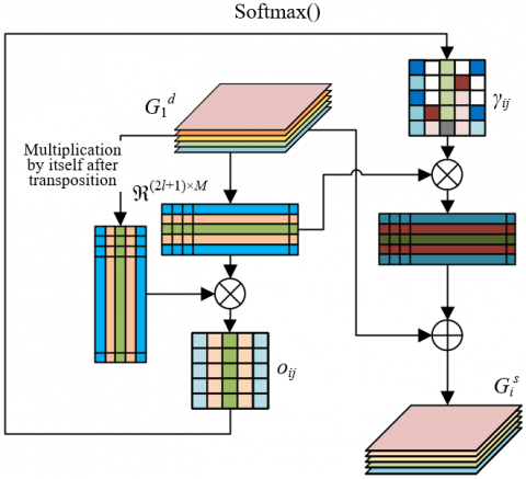
Figure 3. Design of the attention mechanism at the feature level
After the convolution process of the CNN, the feature channels of the deep-level feature map fused can be characterized by the potential features that are correlated. In order to obtain effective information that is conducive to the identification and classification of Alzheimer’s disease based on the central slices in the brain MRI images, the attention mechanism was introduced from the feature level to calculate the potential feature correlation coefficients between the slices. Figure 3 shows the design principle of the attention mechanism at the feature level.
The feature map G1d is transformed into ℜ(2l+1)×M(M=P×Q), and G1d and the transpose of G1d go through matrix multiplication. Suppose that the correlation value of the i-th feature channel and the j-th one on the feature map is denoted as oij. The more similar the two channels, the greater the value of oij, and the larger the weight coefficient assigned. The self-attention coefficient can be calculated based on the softmax(.) function, and the self-attention weight matrix can be further obtained. Suppose that the correlation coefficient between the slice features of the weight matrix is represented by γ $\in$ ℜ(2l+1)×(2l+1), and that the impact of the feature information of the i-th slice on that of the j-th one is represented by the matrix element γij, there is
$\gamma_{i j}=\frac{e^{G_{1 i}^{d} \cdot G_{1 j}^{d}}}{\sum_{j}^{2 l+1} e^{G_{i i}^{d} \cdot G_{1 j}^{d}}}$ (19)
In order to eliminate the impact of noise on the feature information, the max-softmax(.) function can be used to optimize the self-attention coefficient. And there is:
if $\left(\gamma_{i j}>=\gamma_{i j}^{*}\right): \gamma_{i j}=\gamma_{i j}$
else $: \gamma_{i j}=0$ (20)
When γij is smaller than γij*, the impact of noise on the main features can be ignored. Let γij be 0, and at the same time keep the γij greater than the mean value. Further, perform matrix multiplication of G1d by the transpose of γ, and then add the result to G1d in an element-wise manner to obtain the feature map G1r $\in$ ℜ(2l+1)×P×Q, as shown in Eq. (21):
$G_{1}^{r}=G_{1}^{d} \circ \gamma \bullet G_{1}^{d}$ (21)
From the above formula, it can be seen that G1r is the weighted summation of the original features and deep-level features of all brain MRI image slices. In order to improve the presentation of the deep-level feature map, the feature-level attention module was used to extract the potential correlations between the features of the slices. This facilitates the identification and classification of Alzheimer’s disease based on the central slices in the brain MRI images.
In order to effectively cope with the dynamic changes in the features of the slice sequence of the brain MRI image samples, the image features are dynamically adjusted in the time and space domain to achieve a better characterization of the dynamic image samples. In this section, some improvements were made to the constructed deep CNN and a spatio-temporal graph CNN with the attention mechanisms at the regional level and the feature level was built, which made the network model more attentive to the salient channel features and eliminated the impact of some noise features. Figure 4 shows the basic structure of the spatio-temporal graph CNN with dual attention mechanisms.
Figure 4. Basic structure of the spatio-temporal graph CNN with dual attention mechanisms
Spatially, image slices of different frames can be regarded as spatio-temporal maps. Suppose that the vertex on the image slice is denoted as u and that the feature map as YSin. Suppose that the sampling area for the convolution of the target vertex uφi, that is, the set of all first-order pixels adjacent to uφj, is denoted as Ri, and that the weight vector as q. Then, based on the vertex uφi on the image slice of the φ-th frame, the graph convolution operation can be defined as in Eq. (22):
$Y S_{o u t}\left(u_{\phi i}\right)=\sum_{u_{\phi j} \in R_{i}} \frac{1}{C A_{i j}} Y S_{i j}\left(u_{\phi i}\right) q\left(k_{i}\left(u_{\phi i}\right)\right)$ (22)
Since the number of pixels adjacent to each pixel is different, the total number of elements in Ri is not fixed. However, the number of weight vectors in q is fixed, and its weight values can be assigned through the mapping function k. Suppose that the cardinal number of the subset Ri where uφj is located is denoted as CAij, that the size of the convolution kernel as SCu, that the normalized form of the adjacency matrix as LI, and that a learnable weight matrix as WZ. Through transformation of the above formula, the expression of the graph convolution in the spatial dimension can be obtained as follows:
$Y S_{o u t}=\sum_{l}^{S C_{u}} q_{l}\left(Y S_{i n}\left(L I_{l} \bullet W Z_{l}\right)\right)$ (23)
To achieve better identification and classification of Alzheimer’s disease, the attention mechanism modules are then introduced into the spatial graph convolutional layer, so that the model can simultaneously complete the network parameter learning and the connected graph optimization to obtain the graph features that are more suitable for describing Alzheimer’s lesions. Eq. (24) shows the spatial graph convolution expression after the attention modules are introduced:
$Y S_{o u t}=\sum_{l}^{S C_{v}} q_{l}\left(Y S_{i n}\left(L I_{l}^{\prime}+T M_{l}\right)\right)$ (24)
Through comparison of Eq. (23) with Eq. (24), it can be seen that the attention module includes two parts - the data-driven graph matrix LI' and the attention matrix TM. The former is mainly used to complete parameter initialization and update, and the latter is used to improve the adaptability of the model to the dynamic changes in image slices.
Specifically, first use two convolutional layers to map a certain input feature TZ(uφi) into the vectors SC and WC, as shown in Eq. (25). Assuming that the weight matrices corresponding to the two convolutional layers are represented by ξSC and ξWC, respectively, there is:
$\left\{\begin{array}{l}S C_{\phi i}=\xi_{S C} T Z\left(u_{\phi i}\right) \\ W C_{\phi i}=\xi_{W C} T Z\left(u_{\phi i}\right)\end{array}\right.$ (25)
It is assumed that uφi and uφj are in the same time step. Assuming that the inner product symbol is <.>, the inner product of WCφi and SCφj is calculated as follows:
$v_{(\phi, i) \rightarrow(\phi, j)}=\left\langle W C_{\phi i}, S C_{\phi j}\right\rangle$ (26)
The similarity between uφi and uφj is characterized by the inner product v(φ,i)→(φ,j). Assuming that the similarity characterized by the inner product v after normalization is represented by SE, it can be calculated according to Eq. (27):
$S E_{(\phi, i) \rightarrow(\phi, j)}=\frac{\exp \left(v_{(\phi, i) \rightarrow(\phi, j)\quad}\right)}{\sum_{m=1}^{M} \exp \left(v_{(\phi, i) \rightarrow(\phi, j)\quad}\right)}$ (27)
Figure 5. Structure of the constructed neural network for classification
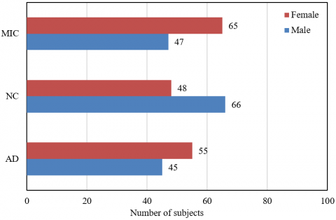
The brain MRI image samples used in this paper can be divided into three types - Alzheimer’s disease (AD), normal control (NC), and mild cognitive impairment (MCI). Table 1 shows the specific information of the brain MRI image samples. There were 100, 114, and 112 samples for AD, NC and MCI, of which 55, 48, and 65 were from females, and 45, 64, and 47 from males. It can be seen that there was little difference in the male-female ratios and the average ages of the samples of these three types. In addition, the results of clinical dementia assessment and mini-mental state examination of all the subjects were also summarized. Figure 6 visually shows the distribution of samples.
Table 1. Information of the brain MRI image samples
|
Type |
AD |
NC |
MCI |
|
Female |
55 |
48 |
65 |
|
Male |
45 |
66 |
47 |
|
Age |
76.52±6.25 |
75.29±5.28 |
78.24±7.29 |
|
CDR |
0.95±0.51 |
0.05±0.28 |
0.48±0.39 |
|
MMSE |
21.58±3.82 |
29.15±1.35 |
25.84±3.28 |
|
Total number of subjects |
100 |
114 |
112 |
Figure 6. Distribution of samples
Considering that the attention mechanisms were introduced into the model from the regional level and the feature level, in order to further study the performance of the two modules, a subdivided ablation experiment was conducted. Table 2 shows the experimental results of the different attention mechanisms.
Table 2. Experimental results of the different attention mechanisms
|
Module type |
Region |
Feature |
|
Dice (brain tissues) |
0.958 |
0.932 |
|
Dice (Alzheimer’s lesions) |
0.795 |
0.821 |
|
Mean |
0.865 |
0.869 |
It can be seen from the table that the attention mechanism module at the regional level performed better in the recognition of normal brain tissues in the brain MRI images. Generally, in the brain MRI image slices visible to the naked eye, the brain tissues of a normal person including white matter, gray matter and cerebrospinal fluid, are more clearly presented and easier to recognize than those of an Alzheimer’s patient.
The attention mechanism module at the feature level has a better effect in the recognition of the lesion areas in the brain MRI images. If the lesion areas are concentrated in a certain region of the brain MRI image slices and the features are relatively concentrated, the loss functions can fully play their roles to ensure the excellent classification performance of the model.
Figure 7 compares the classification performance of different modular architectures. LeNet 1, AlexNet 2, ZFNet 3, VGGNet 4 and ResNet 5 were compared with the proposed model 6, with the accuracy of each model in the binary and ternary classification tasks evaluated based on the collected sample sets. From this figure, it can be seen that the classification precision and the recall rate of the proposed model were the highest, reaching 85.65% and 80.51%.
Figure 7. Comparison of the classification performance of different modular architectures
Figure 8 shows the ROC curves of different network models in different classification tasks. It can be seen that, compared with the other deep learning models, the proposed model had better performance in the classification of brain MRI image sample sets.
Figure 8. ROC curves of different models in different classification tasks
Table 3. Experimental results of different classification tasks
|
Model |
LeNet |
AlexNet |
ZFNet |
VGGNet |
ResNet |
Proposed model |
|
AD/NC |
93.35 |
93.84 |
94.25 |
94.16 |
94.28 |
95.26 |
|
AD/NC |
83.26 |
85.26 |
82.14 |
85.46 |
86.59 |
87.29 |
|
NC/MCI |
79.28 |
76.59 |
78.62 |
79.85 |
81.26 |
82.42 |
|
AD/NC/MCI |
79.28 |
78.35 |
80.29 |
81.34 |
83.29 |
85.24 |
Table 3 shows the experimental results of different classification tasks. It can be seen that the other five models did not perform well in feature extraction after the collected brain MRI images were sliced, mainly because part of the brain MRI image information was lost during the slicing process. The proposed model had better performance in the four classification tasks - AD/NC, AD/NC, NC/MCI and AD/NC/MCI, showing that the model with dual attention mechanisms is more effective in the identification and classification of Alzheimer’s disease than the conventional deep learning models and that the fusion of the brain MRI image information from multiple levels can help obtain more valuable and complete lesion feature information. At the same time, it also verified the effectiveness of the dual attention mechanisms in the classification of brain MRI image sample sets. The introduction of dual attention mechanisms can make the constructed CNN more inclined to learn the salient slice sequence, which further improves its performance in the classification of Alzheimer’s disease.
This paper carried out research on the Alzheimer’s disease identification and classification model based on the CNN with attention mechanisms. In order to find the correlations between the slices in brain MRI images, the attention mechanisms were introduced into the deep CNN from the regional level and the feature level and the brain MRI image information was fused from multiple angles. Then, a spatio-temporal graph CNN with dual attention mechanisms was constructed to eliminate some noise features. Through an experiment, the distribution of the collected brain MRI image samples was analyzed. The performance of the two modules – regional attention and feature attention was further studied, and the experimental results of different attention mechanisms were given. After that, the classification performance of different modular architectures was compared, and the ROC curves of different models in different classification tasks were drawn, proving that the proposed model has better performance in the classification of brain MRI image sample sets.
[1] Liu, J., Li, M., Lan, W., Wu, F.X., Pan, Y., Wang, J. (2016). Classification of Alzheimer's disease using whole brain hierarchical network. IEEE/ACM Transactions on Computational Biology and Bioinformatics, 15(2): 624-632. https://doi.org/10.1109/TCBB.2016.2635144
[2] Li, F., Liu, M., Alzheimer's Disease Neuroimaging Initiative. (2018). Alzheimer's disease diagnosis based on multiple cluster dense convolutional networks. Computerized Medical Imaging and Graphics, 70: 101-110. https://doi.org/10.1016/j.compmedimag.2018.09.009
[3] Fang, C., Li, C., Cabrerizo, M., Barreto, A., Andrian, J., Rishe, N., Loewenstein, D., Duara, R., Adjouadi, M. (2018). Gaussian discriminant analysis for optimal delineation of mild cognitive impairment in Alzheimer’s disease. International Journal of Neural Systems, 28(8): 1850017. https://doi.org/10.1142/S012906571850017X
[4] Zhang, J., Gao, Y., Gao, Y., Munsell, B.C., Shen, D. (2016). Detecting anatomical landmarks for fast Alzheimer’s disease diagnosis. IEEE Transactions on Medical Imaging, 35(12): 2524-2533. https://doi.org/10.1109/TMI.2016.2582386
[5] Schaffer, C., Sarad, N., DeCrumpe, A., Goswami, D., Herrmann, S., Morales, J., Patel, P., Osborne, J. (2015). Biomarkers in the diagnosis and prognosis of Alzheimer’s disease. Journal of Laboratory Automation, 20(5): 589-600. https://doi.org/10.1177%2F2211068214559979
[6] He, R. (2016). Early multidomain intervention to stave off Alzheimer’s disease. Chinese Science Bulletin, 61(32): 3420-3427. https://doi.org/10.1360/N972016-00100
[7] Pardakhti, N., Sajedi, H. (2019). Brain age estimation using brain MRI and 3D convolutional neural network. In 2019 9th International Conference on Computer and Knowledge Engineering (ICCKE), Mashhad, Iran, pp. 386-390. https://doi.org/10.1109/ICCKE48569.2019.8964975
[8] Yang, X., Wang, T., Lei, Y., Higgins, K., Liu, T., Shim, H., Curran, W.J., Mao, H., Nye, J.A. (2019). MRI-based attenuation correction for brain PET/MRI based on anatomic signature and machine learning. Physics in Medicine & Biology, 64(2): 025001. https://doi.org/10.1088/1361-6560/aaf5e0
[9] Devi, C.N., Chandrasekharan, A., Sundararaman, V.K., Alex, Z.C. (2015). Neonatal brain MRI segmentation: A review. Computers in Biology and Medicine, 64: 163-178. https://doi.org/10.1016/j.compbiomed.2015.06.016
[10] He, Q., Roy, S., Jog, A., Pham, D.L. (2015). An example-based brain MRI simulation framework. In Medical Imaging 2015: Physics of Medical Imaging, 9412: 94120P. https://doi.org/10.1117/12.2075687
[11] Tjahyaningtijas, H.P.A. (2018). Brain tumor image segmentation in MRI image. IOP Conference Series: Materials Science and Engineering, 336: 012012. https://doi.org/10.1088/1757-899X/336/1/012012
[12] Patil, H.V., Shirbahadurkar, S.D. (2018). FWFusion: Fuzzy Whale Fusion model for MRI multimodal image fusion. Sādhanā, 43(3): 38. https://doi.org/10.1007/s12046-018-0796-z
[13] Singh, S., Kaushik, S., Vats, R., Jain, A., Thakur, N. (2019). Right ventricle MRI image segmentation of heart. 2019 IEEE 5th International Conference for Convergence in Technology (I2CT), Bombay, India, pp. 1-4. https://doi.org/10.1109/I2CT45611.2019.9033921
[14] Naseem, R., Cheikh, F.A., Beghdadi, A., Elle, O.J., Lindseth, F. (2019). Cross modality guided liver image enhancement of CT using MRI. 2019 8th European Workshop on Visual Information Processing (EUVIP), Roma, Italy, pp. 46-51. https://doi.org/10.1109/EUVIP47703.2019.8946196
[15] Emad, O., Yassine, I.A., Fahmy, A.S. (2015). Automatic localization of the left ventricle in cardiac MRI images using deep learning. 2015 37th Annual International Conference of the IEEE Engineering in Medicine and Biology Society (EMBC), Milan, Italy, pp. 683-686. https://doi.org/10.1109/EMBC.2015.7318454
[16] Molachan, N., Manoj, K.C., Dhas, D.A.S. (2021). Brain tumor detection that uses CNN in MRI. In 2021 Asian Conference on Innovation in Technology (ASIANCON), PUNE, India, pp. 1-7. https://doi.org/10.1109/ASIANCON51346.2021.9544829
[17] Zhang, X., Li, Y., Liu, Y., Tang, S.X., Liu, X., Punithakumar, K., Shi, D. (2021). Automatic spinal cord segmentation from axial-view MRI slices using CNN with grayscale regularized active contour propagation. Computers in Biology and Medicine, 132: 104345. https://doi.org/10.1016/j.compbiomed.2021.104345
[18] Fu’adah, Y.N., Wijayanto, I., Pratiwi, N.K.C., Taliningsih, F.F., Rizal, S., Pramudito, M.A. (2021). Automated classification of alzheimer’s disease based on MRI image processing using convolutional neural network (CNN) with AlexNet architecture. Journal of Physics: Conference Series, 1844: 012020. https://doi.org/10.1088/1742-6596/1844/1/012020
[19] Guan, H., Wang, L., Yao, D., Bozoki, A., Liu, M. (2021, September). Learning transferable 3D-CNN for MRI-based brain disorder classification from scratch: An empirical study. International Workshop on Machine Learning in Medical Imaging, Strasbourg, France, pp. 10-19. https://doi.org/10.1007/978-3-030-87589-3_2
[20] Villain, E., Mattia, G.M., Nemmi, F., Péran, P., Franceries, X., le Lann, M.V. (2021). Visual interpretation of CNN decision-making process using simulated brain MRI. 2021 IEEE 34th International Symposium on Computer-Based Medical Systems (CBMS), Aveiro, Portugal, pp. 515-520. https://doi.org/10.1109/CBMS52027.2021.00102
[21] Folego, G., Weiler, M., Casseb, R.F., Pires, R., Rocha, A. (2020). Alzheimer's disease detection through whole-brain 3D-CNN MRI. Frontiers in Bioengineering and Biotechnology, 8: 534592. https://dx.doi.org/10.3389%2Ffbioe.2020.534592
[22] Yildirim, M., Cinar, A.C. (2020). Classification of Alzheimer's disease MRI Images with CNN based hybrid method. Ingénierie des Systèmes d’Informationj, 25(4): 413-418. https://doi.org/10.18280/isi.250402
[23] Salehi, A.W., Baglat, P., Sharma, B.B., Gupta, G., Upadhya, A. (2020). A CNN model: Earlier diagnosis and classification of Alzheimer disease using MRI. In 2020 International Conference on Smart Electronics and Communication (ICOSEC), Trichy, India, pp. 156-161. https://doi.org/10.1109/ICOSEC49089.2020.9215402