Design and Application of a Slow Feature Algorithm Coupling Visual Selectivity and Multiple Long Short-Term Memory Networks

Slow varying signals, an expression of the invariant, convey the invariant information of the high-level abstract expression of high-frequency input signals. Based on invariant learning, slow feature analysis (SFA) aims to extract the slow attributes of signals, as well as the slow topology between these attributes. The relevant algorithms have been successfully applied in many fields.

In 1989, Hinton [1] became the first to propose the basic concept, fundamental theories, and hypotheses of slow features, and formulated the preliminary theory of slow feature extraction. In 2002, Wiskott and Sejnowski [2] put forward an unsupervised learning algorithm for SFA, which overcomes the lack of samples and constant dimensionality of supervised learning approaches through nonlinear expansion of the feature space. This marks the official establishment of SFA theories and algorithms.

In 2005, Berkes and Wiskott [3] and Wiskott applied the invariant learning results to receptive field learning of complex cells. In 2007, Franzius et al. [4] revealed the properties of invariant on brain cells in the hippocampus, laying the physiological basis for invariant learning. In 2008, Franzius et al. [5] extracted and recognized the invariant features of the position and rotation angle of cartoon fish through SFA, and demonstrated the ability of SFA to extract classification information. Their study provides the theoretical and experimental foundation for applying slow feature algorithms in feature extraction and pattern recognition.

In 2009, Kalmpfl and Maass [6] trained the SFA algorithm with the data generated by Markov chain, and proved that the features extracted by the slow feature algorithm are equivalent to those extracted by feature decay algorithm (FDA), when the small parameter a approximates zero. The results show that invariant feature extraction algorithm is a correct and feasible way to extract features, and the Markov chain applies to slow feature training.

In 2011, Ma et al. [7] provided a kernel-based SFA algorithm, which enables the expansion of the feature space, prevents the computing in high-dimensional space, and applies SFA algorithm in blind signal separation. At this point, the standard SFA finally matured.

In 2012, Luciw et al. [8] presented a hierarchical SFA algorithm to reduce the computing complexity of the standard SFA. Inspired by the divide-and-conquer strategy, their algorithm can ease the computing complexity. But much information may get lost due to the hierarchical structure. Thus, the algorithm does not necessarily extract all global optimal features. In 2013, Escalante-B and Wiskott [9] developed an SFA based on the graph theory (GSFA) to overcome the difficulty in extracting global optimal features, which stems from information loss. The GSFA trains the SFA algorithm with the complex structure of the training images, trying to realize feature extraction according to the complex structure features of the training images.

In 2015, Zhao et al. [10] designed a feature extraction algorithm based on the complex visual information of natural images. From the angle of visual selectivity, the self-designed topologically independent component analysis (TICA) was adopted to extract the slow features of the topological relationship between information in the complex visual space of natural images, revealing the consistency between visual selectivity and slow features.

In 2019, Zhao [11] improved the slow feature algorithm based on visual invariance, and successfully applied the improved algorithm to extract natural image features. In 2020, Zhao [12] developed an improved slow feature algorithm based on visual selectivity, and introduced it successfully to extract features from out-of-focus image series.

In 2020, Zhao [13, 14] improved the SFA algorithm by multiple long short-term memory networks (LSTMs) and spatiotemporal correlations, implemented the algorithm to dynamic forecast of particulate matter 25 (PM25), and demonstrated the excellent prediction ability of the LSTM-improved algorithm.

In recent years, the SFA algorithm has achieved desired effects in various fields, ranging from human behavior recognition [14-16], blind signal analysis [7, 17], dynamic monitoring [18], three-dimensional (3D) feature extraction [19], and multi-person path planning [20]. Great progress has been realized on the theories and applications of SFA. However, there remain two defects with traditional SFA: (1) The expansion of polynomial basis function lacks the support of visual computing theories for primates; (2) The expansion of polynomial basis function cannot learn the uniform, continuous long short-term features through selective visual mechanism. To solve the defects, this paper designs and implements a slow feature algorithm coupling visual selectivity and multiple LSTMs.

1.png

3.4 BELS algorithm

Step 1. Initialize $k=$ get_length $\left(\right.$ Visual_sub_set $\left.\left\{p_{-} a d d\right\}\right) / 2$, and extract subset Visual_sub_set{p_add, k} from the normalized Visual_sub_set, where get_length(*) is the number of elements in set *. The K value is initialized as half of the length of Visual_sub_set{p_add}. The K randomly selected elements from Visual_sub_set are grouped into Visual_sub_set{p_add, k}.

Step 2. Using K-subset generation algorithm to randomly choose k elements from normalized Visual_sub_set, and group them into a subset Visual_sub_set{p_add, k}. Then, sequentially import Visual_sub_set{p_add, k, $\lambda$1}, Visual_sub_set{p_add, k, $\lambda$2} , Visual_sub_set{p_add, k, $\lambda$3}, and Visual_sub_set{p_add, k, $\lambda$4} to algorithms F_LSTM, O_LSTM, P_LSTM, and D_LSTM, thereby predicting parameters λ₁, λ₂, λ₃, and λ₄ and obtaining visual selectivity parameters λ_f, λ_o, λ_p, and λ_d. The visual selectivity parameters are thereby predicted.

Step 3. Normalize parameters based on visual selectivity, using contribution-based normalization method (2). In this way, the normalized parameters λ_f, λ_o, λ_p, and λ_d are obtained.

Step 4. Output the predicted parameter vector α=(λ_f, λ_o, λ_p, λ_d) of Gabor basis functions, and normalize the relevant count relation_s=0. Given that $\forall \beta=(\bar{\lambda} f, \bar{\lambda} o, \vec{\lambda} p, \bar{\lambda} d) \in$ Visual_sub_set(p_add). If Correlation value $\geq \gamma$, then relation_s++, where γ=0.8 is a preset threshold for correlation. Traverse the entire Visual_sub_set(p_add) to compute the correlation coefficient. If $relation_{s} \leq \theta, \theta=\rho \times$ len $\left(\right.$ Visual_sub_set $\left.\left(p_{-} a d d\right)\right)$ , vector $\alpha$ is not related to set Visual_sub_set(p_add). Then, K should be increased by a step length δ, i.e., $k=k+\sigma$ and $k \leq$ len (Visual_sub_set $\left(p_{-}\right.$add $\left.)\right)$, with δ be a parameter controlling the step length, which is measured through experiments. After that, jump to Step 2. Otherwise, go to Step 5.

Step 5. Output prediction parameter α=(λ_f, λ_o, λ_p, λ_d) to Visual_sub_set(p_add).

3.5 Approximate orthogonal pruning based on Lipschitz condition (Lipschitz_Orthogonal_Pruning_Method, LOPM)

In series Visual_sub_set $=\left\{\gamma(i) \mid \gamma(i)=\left(\lambda_{f}^{i}, \lambda_{o}^{i}, \lambda_{p}^{i}, \lambda_{d}^{i}\right), \mathrm{i}=1,2,3, \ldots, \mathrm{M}, \ldots, \mathrm{N}\right\}$, the first M elements are basis functions extracted by myTICA, and the elements M+1 to N are the expanded basis functions predicted by our algorithm. Let $(\mu, \Sigma)$ be the mean and covariance of samples, respectively; $\forall \beta, \bar{\beta} \in$ Visual_sub_set $; \alpha=\left\{\lambda_{f}^{*}, \lambda_{o}^{*}, \lambda_{p}^{*}, \lambda_{d}^{*}\right\}$ be the basis function parameter vector predicted by the LSTM algorithm.

This paper proposes the LOPM to ensure that the predicted basis function α and the functions in the set Visual_sub_set have similar, uniform, and continuous visual features.

According to Lipschitz consistency [23-25], the following inequalities can be obtained:

$\left\{ \begin{align}  & D(Gabor(\alpha ),Gabor(\beta ))\le L\times D(\alpha ,\beta ) \\ & \alpha \le Max\left\{ \mu +\alpha \Sigma  \right\} \\\end{align} \right.$

Since

$D(\alpha ,\beta )\le Max(D(\alpha ,\beta ),D(\beta ,\bar{\beta }))$

When $\bar{L}=\operatorname{Max}(D(\alpha, \beta), D(\beta, \bar{\beta}))$, the finetuning parameter of consistency $\eta=\frac{D(\alpha, \beta)}{D(\alpha, \beta)+D(\beta, \bar{\beta})}$ . If,

$L=\left\{ \begin{matrix}   \bar{L}\ \ \eta \ge \xi   \\   \bar{L}+\eta \ \eta <\xi \ \ \   \\\end{matrix} \right.$

where, ξ is a random small integer preventing overconvergence of the elements in the set Visual_sub_set; Visual_sub_set; $\quad L<<$ D(Visaul_sub_set $(k 1)$, Visual_seb_set $(K 2))$ ;$k 1 \neq K 2, k 1, k 2 \leq$ length $($ Visaul_sub_set $)$.

Then, there must be:

$D(Gabor(\alpha ),Gabor(\beta ))\le L\times D(\alpha ,\beta )$    

Hence, the value of L is determined, and the Lipschitz consistency is basically guaranteed. In this case, function D is introduced to measure the block distance between two vectors:

$D(\alpha ,\beta )=\left| \lambda _{f}^{\alpha }-\lambda _{f}^{\beta } \right|+\left| \lambda _{o}^{\alpha }-\lambda _{o}^{\beta } \right|+\left| +\left| \lambda _{p}^{\alpha }-\lambda _{p}^{\beta } \right|+\left| \lambda _{d}^{\alpha }-\lambda _{d}^{\beta } \right| \right|$  

If $\langle\alpha, \beta\rangle \leq \varepsilon$, vector α is similar to vector β, carry out pruning and retain β; otherwise, add α to set Gabor_set. Note that ε is pruning coefficient, a random small integer controlling the degree of pruning.

Innovation 4. Invariant feature formation

The original SFA algorithm extracts only the PCA features of the natural image, failing to extract slow features from out-of-focus image series or the spatial topology between these features, using the visual computing theory of natural images.

2.png

Figure 2. Feature forest reflecting the visual invariance of the natural out-of-focus image series

Note: tree(m), m=1,2,3,… is the m-th series feature of the out-of-focus image series in the visual space. It is designed according to the global parallel and local serial processing mechanism of visual information of primates, with the aim to facilitate parallel algorithm design.

Inspired by the theory on the consistency of visual selectivity of primates, it is certain that the Gabor basis functions satisfy the consistency of visual selectivity in the complex visual space Visual_sub_set, which corresponds to the target out-of-focus image series. Due to the uniformity and continuity (or invariance) of the four visual parameters f, o, p, and d of basis functions determine the number of basis function spaces and the spatial topological relationship of the out-of-focus image series, as well as the consistency between the type of basis functions in the basis function family and spatial topology.

Through the above improvement, the feature forest can be constructed to reflect the visual invariance of the out-of-focus image series, based on the improved SFA architecture (Figure 2).

To sum up, the slow features of the out-of-focus image series can be expressed as:

$IS=\{tree(m)\ |m=1,2,3...\}$     (5)

$tree(m)\ =\{(index(m,j),gabor(m,j))\}$    (6)

where, m is the visual space basis; j is the position of an element in m, j=1,2,3,…,360. In the IS matrix, the columns have frequency selectivity, and the rows have direction angle selectivity. The elements are ranked in ascending order, with the direction angle falling in [1°, 360°]. Hence, the features can be described by the following matrix.

Table 2. Feature matrix index (each row contains 360 features)

In the feature matrix index, 1 means the receptive field exists at that position; otherwise, the receptive field does not exist at that position. Each node index(i,j) contains the corresponding gabor(i,j) function. These functions form a feature matrix (Tables 2 and 3).

Table 3. Receptive fields corresponding to GMindex

5.1 Image set generation and display

Table 4. Affine transform parameters (the last column is for comparison)

Type	Parameters (rotation angle, number of translation pixels, and scaling factor)
Rotation	0.1	0.3	0.5	0.7	1	5
Translation	1	3	5	7	9	9
Scaling	1/8	1/4	1/2	2	3	4

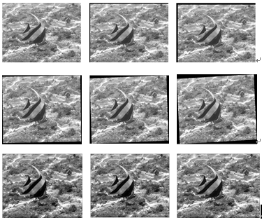
According to the previous theoretical analysis, out-of-focus images can be approximated through the affine transform of original clear images. Hence, 1,000 images are selected from INRIA Holidays dataset, and subjected to affine transform using the parameters in the first five columns of Table 4, producing an image set of 15,000 images. The first 12,000 images were allocated to the training set, and the latter 3,000 into the test set. Each set contains 1,000 original images. Figure 4 shows the samples from the experimental image set.

4.png

Figure 4. Samples from the experimental image set based on INRIA holidays dataset

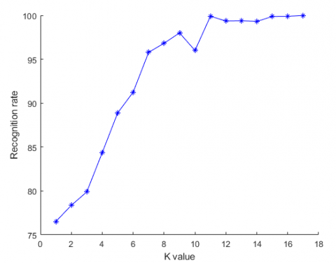
5.2 Relationship between initial K and BELS performance

In our algorithm, the K value determines the visual selectivity consistency of the predicted basis functions. It also bears on the prediction and computing performance of the BELS. This parameter could be configured adaptively according to the learning results. Therefore, the initial K value determines the prediction performance and execution process of the BELS. The selection of K value is critical to whether the predicted basis functions can learn the global distribution features of set Visual_sub_set(i). Experiments show that the initial K should satisfy $K=\operatorname{Min}($ length $($ visual_sub_set $(i), i=1,2,3, \ldots, N) / 2)$. Through random sampling, the K-subset generation algorithm collects K elements from set visual_sub_set(i), forming a new set Visual_sub_set(i,λ_t) with t$\in$(λ_f, λ_o, λ_p, λ_d).

On the training set, the relationship of initial K and the prediction performance of the BELS is shown in Table 5.

With the growth of initial K, more basis functions in Visual_sub_set(i) participate in the prediction, and the learnable global visual features are enhanced. Meanwhile, the predicted basis function $\alpha$ has stronger global features of the basis function set Visual_sub_set(i), and exhibit a more uniform and continuous visual selectivity. The results of RMSE, MAE, and MAPE all gradually decrease. Therefore, the BELS can achieve a very strong prediction performance.

5.png

Figure 5. Relationship between k value and BELS performance

The K value has the following correspondence with K: $K\left(k_{-}\right.$value $)=\frac{N}{2}+\left(k_{-}\right.$value $\left.-1\right) \times d$, where d=1/38 is the tolerance; N is the size of Visual_sub_set(i).

As shown in Figure 5, with the growth of initial K, the BELS witnesses an improvement in prediction performance; the predicted basis function $\alpha$can better learn and inherit the global features of elements in set Visual_sub_set(i), and achieve a more uniform and continuous visual selectivity. Therefore, the recognition performance of our algorithm increases with the K value.

5.3 Relationship between initial δ and prediction performance

In our algorithm, the growth rate of K is described by parameter δ:

$\left\{ \begin{matrix}   \delta ={{\delta }_{0}}  \\   {{\delta }_{t}}={{\kappa }_{t}}-{{k}_{t-1}}  \\   {{k}_{t+1}}={{k}_{t}}+{{\delta }_{t}}  \\\end{matrix} \right.$     (10)

This parameter is an integer that determines the learning rate of the BELS. Hence, the initial value of this parameter is correlated with the prediction performance of the algorithm. The relationship between parameter δ and parameter K on the training set is shown in Table 6.

As initial δ increases from -5 to 5, the K value increases, and the predicted basis function $\alpha$ can better learn and inherit the global features of elements in set Visual_sub_set(i), and achieve a more uniform and continuous visual selectivity. That is, the BELS acquires stronger learning ability. Thus, the greater the K value, the smaller the changes of RMSE, MAE, and MAPE.

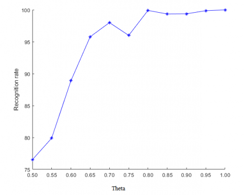
5.4 Relationship between initial θ and prediction and recognition performance

In this paper, parameter \theta \in[0,1] describes the uniformity and continuousness of visual features between predicted basis function $\alpha=\left\{\lambda_{f}^{*}, \lambda_{o}^{*}, \lambda_{p}^{*}, \lambda_{d}^{*}\right\}$ and basis function $\beta \in$ Visual_sub_set(i). Table 7 shows the relationship between $\theta \geq 0.5$ and the prediction ability of our algorithm.

Table 7. Relationship between parameter θ and our algorithm’s prediction performance

As parameter θ increases from 0.5 to 0.8, the uniformity and continuousness of visual features improve between basis functions α,β. The visual selectivity of predicted basis function α are uniform and correlated with those of the basis function set Visual_sub_set(i). The greater the value of θ, the predicted basis function $\alpha$ can better learn and inherit the global features of elements in set Visual_sub_set(i), achieve a more uniform and continuous visual selectivity, and reduce the error with Visual_sub_set(i). Thus, the greater the θ value, the smaller the changes of RMSE, MAE, and MAPE.

6.png

Figure 6. Relationship between parameter θ and our algorithm’s prediction performance

As shown in Figure 6, when parameter θ increases from 0.5 to 0.8, the uniformity and continuousness of visual features improve between basis functions α,β; the predicted basis function $\alpha$ can better learn and inherit the global features of elements in set Visual_sub_set(i), achieve a more uniform and continuous visual selectivity, and acquire a stronger classification ability. Meanwhile, the algorithm becomes more excellent in classification, at the cost of rising time complexity. Overall, our algorithm has the best prediction effect at θ=0.8.

5.5 Distribution consistency between predicted basis function and basis function set

Using the above optimal parameters, our algorithm is executed on the training set. The distribution of the predicted basis function$\alpha=\left\{\lambda_{f}^{*}, \lambda_{o}^{*}, \lambda_{p}^{*}, \lambda_{d}^{*}\right\}$ and that of $\forall \bar{\beta}, \bar{\beta} \in$ Visual_sub_set $(i)$ are obtained as shown in Figure 7.

7.png

Figure 7. Distribution of the predicted basis function and basis function set

The global visual selectivity of basis function set Visual_sub_set(k3) is learned by the basis function α predicted by the BELS. The predicted basis function α achieves a strong consistency in visual selectivity with the set. In terms of visual selectivity, the predicted basis function has a small intra-class dispersion with its family Visual_sub_set(k2), and a large between-class dispersion with the other families Visual_sub_set(k1) and Visual_sub_set(k3). This satisfies the theoretical requirements of uniform and continuous visual selectivity within the class, and the differential visual selectivity across classes, and demonstrates the visual selectivity features of primates. Hence, our BELS can generate basis functions consistent in visual selectivity, and uniformly distributed across families.

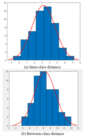
5.6 Feasibility of our algorithm

Using k=N/2, σ=1, and θ=0.75, our algorithm is applied to the training set. The intra-class and between-class distribution performance of our algorithm is recorded in Figure 8.

Our algorithm is improved from the original SFA algorithm with the aid of BELS and LOPM. In visual selectivity, the predicted basis function has a strong uniformity and consistency with the basis function set Visual_sub_set(k3). Hence, the predicted basis function α has a relatively small intra-class dispersion and a relatively large between-class dispersion. Under k=N/2, σ=1, θ=0.75, and threshold of 6, the receiver operating characteristic (ROC) curve shows that the recognition rate of our algorithm was 99.98%, and the false accept rate (FAR) and false reject rate (FRR) were both smaller than 0.02%, indicating the strong classification ability of our approach.

8.png

Figure 8. Intra-class and between-class distribution performance of our algorithm

5.7 Superiority of our algorithm

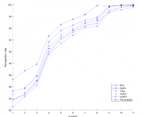
Using k=N/2, σ=1, and θ=0.75, our algorithm is compared with SFA [1], GSFA [8], TICA [9], myTICA [10], and mySFA [11] (Figure 9).

9.png

Figure 9. Recognition performance of different algorithms

Based on these conventional approaches, our algorithm replaces the polynomial method of basis function expansion in the original SFA with the BELS, such that the predicted basis function α is highly uniform and continuous with the basis function set Visual_sub_set(i) in terms of visual selectivity. In addition, LOPM pruning technique is adopted to realize the Lipschitz consistency condition of the predicted basis function. As a result, under k=N/2, σ=1, and θ=0.75, the basis function α predicted by our algorithm has strong uniformity and continuity, and realizes uniform and continuous visual selectivity. Besides, the basis function boasts a small intra-class dispersion and a high between-class dispersion. These results show that our algorithm has a stronger classification effect than conventional approaches.