Chao Liu | Jing Yang* | Weinan Zhao | Yining Zhang | Cuiping Shi | Fengjuan Miao | Jinsong Zhang
© 2021 IIETA. This article is published by IIETA and is licensed under the CC BY 4.0 license (http://creativecommons.org/licenses/by/4.0/).
OPEN ACCESS
Face images, as an information carrier, are rich in sensitive information. Direct publication of these images would cause privacy leak, due to their natural weak privacy. Most of the existing privacy protection methods for face images adopt data publication under a non-interactive framework. However, the $\varepsilon$-effect under this framework covers the entire image, such that the noise influence is uniform across the image. To solve the problem, this paper proposes region growing publication (RGP), an algorithm for the interactive publication of face images under differential privacy. This innovative algorithm combines the region growing technique with differential privacy technique. The privacy budget $\varepsilon$ is dynamically allocated, and the Laplace noise is added, according to the similarity between adjacent sub-images. To measure this similarity more effectively, the fusion similarity measurement mechanism (FSMM) was designed, which better adapts to the intrinsic attributes of images. Different from traditional region growing rules, the FSMM fully considers various attributes of images, including brightness, contrast, structure, color, texture, and spatial distribution. To further enhance algorithm feasibility, RGP was extended to atypical region growing publication (ARGP). While RGP limits the region growing direction between adjacent sub-images, ARGP searches for the qualified sub-images across the image, with the aid of the exponential mechanism, thereby expanding the region merging scope of the seed point. The results show that our algorithm can satisfy $\varepsilon$-differential privacy, and the denoised image still have a high availability.
face image publication, interactive framework, differential privacy, region growing, growth rule
Since its nascency, facial recognition has attracted much attention for the intuitiveness, uniqueness, and privacy of face images. The public cautiously enjoy the convenience of facial recognition, while worrying about whether their privacy and rights will be violated someday. With the commercialization of facial recognition, consumers are calling for effective regulation of the technology. Many scholars and organizations have worked to promote relevant legislations. Against this backdrop, the United States Government Accountability Office (U.S. GAO) released two reports: Facial Recognition Technology: Federal Law Enforcement Agencies Should Better Assess Privacy and Other Risks, and Facial Recognition Technology: Privacy and Accuracy Issues Related to Commercial Uses. In China, the Public Research Report of Facial Recognition Applications shows that, more than 60% of the respondents feel that facial recognition has been misused, and over 30% expressed that they have suffered privacy leak or financial loss due to the misuse of facial recognition. Therefore, information technology is a mixed blessing. How to make good use of the technology is a worldwide concern. Owing to the rapid development of information technology and multimedia technology, it is increasingly easy to acquire and share digital face images. Users can upload the photos in their mobile phones or digital cameras to social network platforms like Twitter, Pinterest, LinkedIn, or WeChat. Statistics have shown that more than 3.2 billion face images are shared by users each day on the major social network platforms across the globe. Besides, countless face images are generated from videos. These digital images contain lots of sensitive personal information. If they are collected and analyzed by malicious third-parties, privacy leak and other losses will be beyond measure [1].
In related reports, some stakeholders express concerns about the privacy issues related to the commercial use of facial recognition. The technology may publicly identify and track people without being noticed by them, and may collect, use, and share their personal data. However, some working in the industry argue that facial recognition will not bring new or special privacy risks, and the risks of the technology are controllable.
The National Telecommunications and Information Administration (NTIA) once organized a test on multiple parties. Some participants worried that facial recognition may threaten personal privacy, because it reduces the anonymity of individuals in public or commercial locations (such as pavement or stores). The participants also expressed the concern that facial recognition may be used to individuals in public, and erode personal privacy. Industry insiders revealed that facial recognition has not been widely used to track consumers in business environments.
The Center for Democracy and Technology announces that most people are willing to be facially identified in public by some people or enterprises. But they do not want their faces to be linked with their names, not to mention associating their faces with other data, such as network behavior, and travel plan. If facial technology is widely adopted in public, and if the recognized faces are shared between enterprises, the consumer movement from one place to another will be tracked any time by a network of cameras. A representative of World Privacy Forum wore that, most consumers will find their privacy be violated, if their activities are tracked by security cameras for marketing. Similarly, the staff of the Federal Trade Commission reported that, consumers will face higher privacy risks, if enterprises start tracking consumers in stores, using collected digital images.
Another widely concerned issue is that consumers will find it impossible to opt out if facial technology is popularized, even if they are notified of the right to reject facial recognition. In many cases, facial recognition is applied to commercial identity recognition or verification, without the knowledge or consent from consumers. This issue has been noticed by some industry trade organizations, which remain cautious about using facial recognition without informed consent from consumers. Computer and Communications Industry Association suggested that, when an enterprise matches face images with names and curriculum vitae through facial recognition, the whole process should remain transparent, and the relevant parties must be given the right to opt out.
Market surveys, patent data, as well as the growing participation in the Facial Recognition Vendor Test (FRVT) organized by the National Institute of Standards and Technology (NIST), indicate that a rising number and types of enterprises are adopting facial recognition. Facial recognition often relies on the acquisition of massive face images (face image databases). Focusing on the massive personal data in such databases, privacy protection organizations, government agencies, the academia, and some industry representatives have expressed concerns over the collection, use, and sharing of personal data by commercial entities.
Face image databases can be sold or shared by all parties, but the selling range remains unknown. The data associated with facial recognition may be sold or shared, often without the knowledge or consent from the affected parties. In recent years, there is a surge in the total amount of personal data collected and shared by resellers and other enterprises, which exacerbates the public concern over this issue.
Privacy is a word with emotional color. Different people have different understandings of this word. According to the International Organization for Standardization (ISO), privacy refers to the features that distinguish individuals or groups from other individuals and groups. Different countries have different legal definitions of privacy. The definition of privacy also varies with objects (individuals, enterprises, governments, etc.). For digital images, sensitive information can be a specific person or object in the original image, a face or fingerprint, embedded information (the location and creation time of the image), or the region of interest (ROI) in the eyes of the image owner. How to publish and analyze images without disclosing sensitive information is the main purpose of privacy protection.
The above privacy issues can be solved through image data query under privacy protection. For the image data released on the social network, the privacy can be usually protected by k-anonymity, access control, and privacy encryption. Fung et al. [2] and Xiao and Tao [3] proposed the k-same method under the anonymization mechanism. Their method anonymizes the published grayscale image, reducing the probability that the attacker re-identifies the user with the published image to less than 1/k. However, the traditional anonymization mechanism has a prominent defect: Before data processing, researchers must set lots of prior conditions for the attacker’s background knowledge and attack models. But these conditions are not fully established in reality. For example, Li et al. [4] relied on access control to restrict user access to social network images, and to control the number of transfers and accesses of the images published on the social network. Despite realizing the goal of privacy protection, the access-oriented protection is merely a superficial privacy protection approach for images. If the attacker has a certain background knowledge, he/she will be able to acquire user images and the relevant privacy information. Terrovitis et al. [5] carried out same-state encryption of the grayscale image to prevent the re-identification of the communication process. Nevertheless, the data encryption algorithms are developed based on some assumptions of the attacks. The existing algorithms are quickly phased out, due to the continuously updating attack modes. Sweeney [6] revealed that attackers can identify sensitive personal information (diseases, and address) from anonymous images on Facebook by deriving the social security number (SSN) of the people in the anonymous images from the extra Friendster feature of Facebook. So, is there any technique that can protect personal privacy in spatial data without the background knowledge of an attacker? This is the focus of image data publication based on differential privacy.
In 2006, Dwork [7] invented differential privacy, which disturbs sensitive data by adding noise to the output. Differential privacy can limit the further reasoning ability of the attacker by hiding the impact of a single record, i.e., the output probability of the same result does not change significantly, whether the record is in the dataset. Therefore, differential privacy does not make any assumption for any potential attacker’s background knowledge. This is better than other privacy protection technologies. Dwork further investigated differential privacy in a series of theses [8-12], and proposed its implementation mechanism [13, 14]. McSherry [15] pointed out that the differential privacy algorithm for complex privacy issues need to satisfy two combined features: sequence combination and concurrent combination. In recent years, differential privacy is mainly applied in data publication. To protect data publication with differential privacy, the main issues is to ensure the accuracy of the released data or query results, while fulfilling the conditions of differential privacy. The relevant research mainly focuses on the publication mechanism and algorithm complexity. The main research approach is quantification based on calculation theory and learning theory. Based on the realization environment, data publication protected by differential privacy can be divided into interactive data publication and non-interactive data publication [13]. The representative interactive data publication (query) methods are as follows: Roth and Roughgarden [16] presented a Median algorithm that can respond to multiple queries. Hardt and Rothblum [17] developed a private multiplicative weights (PMW) mechanism that increases the number of queries. Gupta et al. [18] put forward a universal iterative dataset creation (IDC) framework. Fan and Xiong [19] designed a FAST algorithm based on filtering and adaptive sampling. Kellaris et al. [20] designed a flow data publication algorithm with an unlimited number of queries. When it comes to non-interactive data publication, histogram publication is the most widely adopted technique. The representative strategies include Xiao et al.’s [21] Privelet algorithm, Xu et al.’s [22] Noise First and Structure First algorithms, Li et al.’s [23] matrix mechanism, and Yuan et al.’s data- and workload-aware (DAWA) algorithm [24]. Due to the complexity of image data, the research of sensitive information in the images protected by differential privacy is still in the exploratory stage.
The real domain matrix is a common representation of images. Any pixel in the image can be mapped to a value at the corresponding position of the two-dimensional (2D) matrix. The most direct approach is to add a Laplace noise to all values in the matrix. Although this approach can satisfy ε-differential privacy, the disturbed image will be excessively distorted and weakly available. Fourier transform and wavelet transform are often adopted to compress images. Zhang et al. [25] proposed an image compression method based on discrete Fourier transform, which adds corresponding Laplace noise to the compressed image. Despite reducing the noise error, their method introduces reconstruction error to image compression. Considering the noncorrelation between data in image matrix, Nissim et al. [26] converted the grayscale matrix into a one-dimensional (1D) sequential data flow through image segmentation, modeled the data flow with sliding window model, and dynamically distribute privacy budget based on the data similarity between adjacent sliding windows. In this way, the privacy protection of images is achieved. However, this highly feasible approach faces two problems: the overall operation is confined in the 1D space, and Laplace noise covers the entire image.
2.1 Differential privacy
Dalenius pointed out a problem with the statistics database: No one should get any information about any person by accessing the database. However, absolute privacy protection is impossible due to background knowledge. Differential privacy circumvents this problem, and pursues relative privacy protection, trying to limit any possible privacy leak to the range of a small multiplier factor. Note that severe leaks may still occur, but will not be caused by whether a certain data exists in the database.
Face images, as a carrier of information, are usually stored and transmitted using three-dimensional (3D) matrices (i.e., a color image can be described as three 2D matrices red R, greed G, and blue B). For simplicity, the 3D image matrix is normalized to obtain the corresponding 2D grayscale matrix. Then, image X can be represented as a 2D matrix Xmn, where m and n are the number of rows and columns of the matrix, respectively:
$X_{m n}=R_{m n} \times 0.299+G_{m n} \times 0.587+B_{m n} \times 0.114$ (1)
Adjacent datasets are an important concept of differential privacy. In fact, the concept comes from the basic operations of sets. The main set operation adopted for adjacent datasets is the operation of symmetric difference $\oplus$. In the set operation formula $\mathrm{T}=\mathrm{R} \oplus \mathrm{S}=(\mathrm{RUS})-(\mathrm{R} \cap \mathrm{S})$, T contains the elements in set R but not in set S, and the elements in set S but not in set R. The number of different elements between the two sets can be calculated by $\Delta=|R \oplus S|$. Before giving a formal definition of differential privacy, it is necessary to define the adjacent datasets of face image X.
Definition 1. Adjacent datasets of face image
For a given image X, the grayscale matrix Xmn can be obtained by normalizing the image. Then, there exists $\mathrm{X} \mid \mathrm{X}_{\mathrm{mn}}=\left[\begin{array}{ccc}\mathrm{x}_{11}, \mathrm{x}_{12}, & \cdots & \mathrm{x}_{1 \mathrm{n}} \\ \vdots & \ddots & \vdots \\ \mathrm{x}_{\mathrm{m} 1}, \mathrm{x}_{\mathrm{m} 1}, & \cdots & \mathrm{x}_{\mathrm{mn}}\end{array}\right]$, where xij in matrix Xmn represents the grayscale of the corresponding element. If there exists an X' with only one element difference from X, $\left|X-X^{\prime}\right|=x_{i j}(1 \leq i \leq m, 1 \leq j \leq n)$, then X and X' are adjacent datasets.
Definition 2. Differential privacy
For a given random algorithm M of image data publication, with the output range of Range(M), the algorithm can provide ε- differential privacy, if its arbitrary outputs on two adjacent grayscale images X and X' satisfy:
$\operatorname{Pr}[M(X) \in S] \leq \exp (\varepsilon) \times \operatorname{Pr}\left[M\left(X^{\prime}\right) \in S\right]$ (2)
where, ε is typically a small positive number that balances privacy with accuracy. If ε is small, the privacy is high and accuracy is low. The inverse is also true. Normally, ε is selected by the user by executing a privacy policy. When the adjacent datasets vary by only one record, the algorithm satisfies ε-differential privacy. When the adjacent datasets vary by k records, the algorithm satisfies kε-differential privacy.
To realize differential privacy, a certain amount of random noise needs to be added to the query results. Intuitively, the magnitude of the additive noise should surpass the maximum impact of a single record on the output. Therefore, the noise level is closely related to the global sensitivity of the corresponding query function.
Definition 3. Global sensitivity
Let Q be a random query function meeting $Q: D \rightarrow R^{n}$. Then, the global sensitivity of Q can be expressed as:
$\Delta Q_{G S}=\max _{X, X^{\prime}}\left\|Q(D)-Q\left(D^{\prime}\right)\right\|_{\rho}$ (3)
Global sensitivity can indeed be applied to all methods of differential privacy. But some functions have a relatively high global sensitivity. In this case, lots of noise need to be added to ensure privacy. Then, the balance between information availability and privacy will be undermined after privacy protection. To solve the problem, Nissim et al. proposed the concept of local sensitivity [26]. Nissim held that, for the same function, it is possible to predict the distribution feature of a subset d of a dataset D with a high global sensitivity. Under the effect of the prediction result, a relatively small local sensitivity could be obtained specifically for d. The local sensitivity, and its relationship with global sensitivity are explained below.
Definition 4. Local sensitivity
Let Q be a random query function meeting $Q: d \rightarrow R^{n}(d \in D)$. Then, the local sensitivity of Q can be expressed as:
$\Delta Q_{L S}=\max _{X , X^{\prime}}\left\|Q(d)-Q\left(d^{\prime}\right)\right\|_{\rho}$ (4)
$\Delta Q_{G S}=\max \left(\Delta Q_{L S}\right)$ (5)
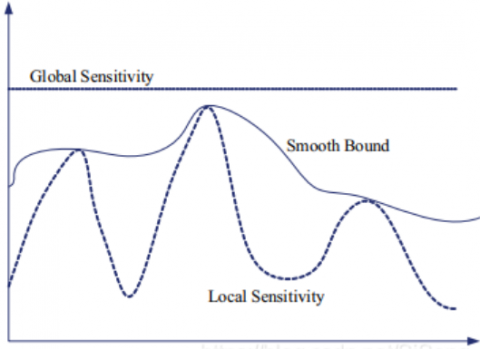
Note that any dataset d with predictable distribution feature faces the risk of privacy leak. To solve the potential privacy leak of local sensitivity, the smooth upper bound is defined for local sensitivity.
Definition 5. Smooth upper bound
For a dataset d and its adjacent dataset d’, if the local sensitivity of function Q is $\Delta \mathrm{Q}_{\mathrm{LS}}$, the function $\mathrm{S}: \mathrm{d} \rightarrow \mathrm{R}^{\mathrm{n}}$ satisfying $\mathrm{S}(\mathrm{d}) \geq \Delta \mathrm{Q}_{\mathrm{L} \mathrm{s}}$ and $\mathrm{S}(\mathrm{d}) \leq \mathrm{e}^{\beta} \mathrm{S}\left(\mathrm{d}^{\prime}\right)(\beta>0)$ is the $\beta$- smooth upper bound of the local sensitivity of function Q.
Any function S meeting Definition 5 can be treated as a smooth upper bound. During the use, the local sensitivity $\Delta \mathrm{Q}_{\mathrm{LS}}$ is substituted to function S to obtain the corresponding smoothness sensitivity, and then derive the final Laplace noise. Figure 1 shows the relationship between the smooth upper bound and local sensitivity.
Figure 1. Smooth upper bound of local sensitivity
Theorem 1. Laplace mechanism
Let Q be a query series of the length d. The random algorithm M receives database D and outputs the following vector that satisfy ε-differential privacy:
$\mathrm{M}(\mathrm{D})=\mathrm{Q}(\mathrm{D})+<\operatorname{Lap}_{1}\left(\Delta \mathrm{Q}_{\mathrm{LS}} / \varepsilon, \ldots, \mathrm{Lap}_{\mathrm{d}}\left(\Delta \mathrm{Q}_{\mathrm{LS}} / \varepsilon>\right.\right.$ (6)
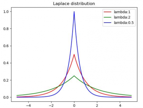
As the most common noise addition mechanism, the Laplace mechanism disturbs the real output by adding the noise generated by Laplace distribution, thereby achieving differential privacy. The probability density function (PDF) of its noise distribution satisfies $f(x \mid \mu, b)=\frac{1}{2 b} e^{\frac{|x-\mu|}{b}}$ (Figure 2).
Figure 2. Laplace PDF
Then, the cumulative probability distribution function can be derived from the PDF in the following manner:
$F(x \mid \mu, b)=\left\{\begin{array}{c}\frac{1}{2} e^{\frac{\mu-x}{b}}, x<u \\ 1-\frac{1}{2} e^{\frac{x-\mu}{b}}, x \geq u\end{array}\right.$
If $\mathrm{x}<\mu$, and $\mathrm{f}(\mathrm{x} \mid \mu, \mathrm{b})=\frac{1}{2 \mathrm{~b}} \mathrm{e}^{\frac{|\mathrm{x}-\mu|}{\mathrm{b}}}$, there exists:
$F(x \mid \mu, b)=\frac{1}{2 b} \int_{-\infty}^{x} e^{\frac{\mu-x}{b}} d x=\frac{1}{2 b} \int_{-\infty}^{x} e^{\frac{x-\mu}{b}} d x$
Suppose $\mathrm{t}=\frac{\mathrm{x}-\mu}{\mathrm{b}}$. We have:
$F(x \mid \mu, b)=\frac{1}{2 b} \int_{-\infty}^{\frac{x-\mu}{b}} b e^{t} d t=\frac{1}{2} \int_{-\infty}^{\frac{x-\mu}{b}} e^{t} d t=\frac{1}{2}\left[e^{t}\right]_{-\infty}^{\frac{x-\mu}{b}}=\frac{1}{2} e^{\frac{x-\mu}{b}}$
Expectation and variance are the two most basic attributes of the probability distribution. For a Laplace distribution function, the expectation and variance $\mu$ and $2 b^{2}$ can be derived by:
Expectation:
$\mathrm{E}(x)=\frac{1}{2 b}\left(\int_{-\infty}^{\mu} x e^{\frac{\mu-x}{b}} d x+\int_{\mu}^{+\infty} x e^{\frac{\mu-x}{b}} d x\right)=\frac{1}{2 b}\left(\int_{-\infty}^{0} b(b t+\mu) e^{t} d t-\int_{0}^{-\infty} b(\mu-b t) e^{t} d t\right)$
$=\frac{1}{2 b} \int_{0}^{-\infty} b((b t+\mu)+(\mu-b t)) e^{t} d t=\int_{-\infty}^{0} \mu e^{t} d t=\mu$
Variance:
$\mathrm{D}(x)=E\left(x^{2}\right)-E^{2}(x)=\frac{1}{2 b}\left(\int_{-\infty}^{\mu} x^{2} e^{\frac{\mu-x}{b}} d x+\int_{\mu}^{+\infty} x^{2} e^{\frac{\mu-x}{b}} d x\right)-\mu^{2}=\frac{1}{2 b}\left(\int_{-\infty}^{0} b\left((b t+\mu)^{2}+(\mu-b t)^{2}\right) e^{t} d t\right)-\mu^{2}$
$=\frac{1}{2 b}\left(\int_{-\infty}^{0} 2 b\left(b^{2} t^{2}+\mu^{2}\right) e^{t} d t\right)-\mu^{2}=b^{2} \int_{-\infty}^{0} t^{2} e^{t} d t=b^{2} \int_{-\infty}^{0} t^{2} d e^{t}=b^{2}\left(\left[t^{2} e^{t}\right]_{-\infty}^{0}-\int_{-\infty}^{0} e^{t} d t^{2}\right)$
$=-2 b^{2} \int_{-\infty}^{0} t d e^{t}=-2 b^{2}\left(\left[t e^{t}\right]_{-\infty}^{0}-\int_{-\infty}^{0} e^{t} d t\right)=2 b^{2}$
Note that $\operatorname{Lap}_{\mathrm{i}}\left(\Delta \mathrm{Q}_{\mathrm{LS}} / \varepsilon\right)(1 \leq \mathrm{i} \leq \mathrm{d})$ is an independent Laplace noise, whose magnitude is positively proportional to $\Delta \mathrm{Q}_{\mathrm{LS}}$, and negatively proportional to $\varepsilon $.
Theorem 2. Exponential mechanism
The exponential mechanism mainly handles the non-numeric outputs of the sampling algorithm. Under any exponential mechanism, the sampling algorithm M satisfies ε-differential privacy if it meets:
$M(X, u)=\left\{r: \mid \operatorname{Pr}[r \in S] \propto \exp \left(\frac{\varepsilon u(X, r)}{2 \Delta u_{L S}}\right)\right\}$ (7)
where, u(X,r) is the scoring function; $\Delta \mathrm{u}_{\mathrm{LS}}$ is the global sensitivity of the scoring function u(X,r); S is the output domain of our algorithm; r is the selected output term of the output domain S. The higher the score of u(X,r), the greater the probability for r being selected as the output.
Corollary 1. Algorithm M in Definition 2 satisfies ε- differential privacy.
Proof: X and X' are adjacent datasets, with $\mathrm{M}(\mathrm{X})=\left(\mathrm{x}_{1}, \mathrm{x}_{2}, \ldots \mathrm{x}_{\mathrm{d}}\right)^{\mathrm{T}}$ and $\mathrm{M}\left(\mathrm{X}^{\prime}\right)=\left(\mathrm{x}_{1}^{\prime}, \mathrm{x}_{2}^{\prime}, \ldots \mathrm{x}_{\mathrm{d}}^{\prime}\right)^{\mathrm{T}}=\left(\mathrm{x}_{1}+\Delta \mathrm{x}_{1}, \mathrm{x}_{2}+\Delta \mathrm{x}_{2}, \ldots \mathrm{x}_{\mathrm{d}}+\Delta \mathrm{x}_{\mathrm{d}}\right)^{\mathrm{T}}$. Without loss of generality, it is assumed that $\mathrm{x}_{\mathrm{i}}=0\left(\mathrm{x}_{\mathrm{i}} \in \mathrm{X}\right)$ and $\rho=1$. It can be calculated that $\mathrm{M}(\mathrm{X})=(0,0, \ldots 0)^{\mathrm{T}}$ and $\mathrm{M}\left(\mathrm{X}^{\prime}\right)=\left(\Delta \mathrm{x}_{1}, \Delta \mathrm{x}_{2}, \ldots \Delta \mathrm{x}_{\mathrm{d}}\right)^{\mathrm{T}}$. When the vector $S=\left(S_{1}, S_{2}, \ldots S_{d}\right)^{T}$ is outputted, it can be seen that:
$\operatorname{Pr}[M(X) \in S]=\prod_{i=1}^{d} \frac{\varepsilon}{2 \Delta Q_{G S}} e^{\frac{\varepsilon}{\Delta Q_{G S}}\left|s_{i}\right|}$
$\operatorname{Pr}\left[M\left(X^{\prime}\right) \in S\right]=\prod_{i=1}^{d} \frac{\varepsilon}{2 \Delta Q_{G S}} e^{\frac{\varepsilon}{\Delta Q_{G S}}\left|\Delta x_{i}-S_{i}\right|}$
$\frac{\operatorname{Pr}[M(X) \in S]}{\operatorname{Pr}\left[M\left(X^{\prime}\right) \in S\right]}=\frac{\prod_{i=1}^{d} \frac{\varepsilon}{2 \Delta Q_{G S}} e^{\frac{\varepsilon}{\Delta Q_{G S}}\left|s_{i}\right|}}{\prod_{i=1}^{d} \frac{\varepsilon}{2 \Delta Q_{G S}} e^{\frac{\varepsilon}{\Delta Q_{G S}}\left|\Delta x_{i}-s_{i}\right|}}=\prod_{i=1}^{d} e^{\frac{\varepsilon}{\Delta Q_{G S}}\left(\left|s_{i}\right|-\left|\Delta x_{i}-s_{i}\right|\right)}=e^{e^{\frac{\varepsilon}{\Delta Q_{G S}}} \sum_{i=1}^{d}\left(\left|\Delta x_{i}-s_{i}\right|-\left|s_{i}\right|\right)}$
Because of inequality $-\left|\Delta \mathrm{x}_{\mathrm{i}}\right| \leq\left|\Delta \mathrm{x}_{\mathrm{i}}-\mathrm{s}_{\mathrm{i}}\right|-\left|\mathrm{s}_{\mathrm{i}}\right| \leq\left|\Delta \mathrm{x}_{\mathrm{i}}\right|$, and $\Delta \mathrm{Q}_{\mathrm{GS}}=\max \left(\sum_{\mathrm{i}=1}^{\mathrm{d}}\left|\mathrm{x}_{\mathrm{i}}-\mathrm{x}_{\mathrm{i}}^{\prime}\right|\right)=\max \left(\sum_{\mathrm{i}=1}^{\mathrm{d}}\left|\Delta \mathrm{x}_{\mathrm{i}}\right|\right)$, we have $\sum_{\mathrm{i}=1}^{\mathrm{d}}\left(\left|\Delta \mathrm{x}_{\mathrm{i}}-\mathrm{s}_{\mathrm{i}}\right|-\left|\mathrm{s}_{\mathrm{i}}\right|\right) \leq \Delta \mathrm{Q}_{\mathrm{GS}}$. Hence, Algorithm M satisfies $\varepsilon$-differential privacy.
Corollary 2. When norm p takes a random value, Algorithm M does not necessarily satisfy $\varepsilon$-differential privacy.
Proof: From the definition of the norm, it can be learned that $\|x\|_{p}$ is a decreasing function with the increase of p. Let $\Delta Q_{G S}^{(p)}=\max _{X, X^{\prime}}\left\|M(X)-M\left(X^{\prime}\right)\right\|_{p}$ be the value of $\Delta Q_{G S}$ under norm p, with $1 \leq \mathrm{p} \leq+\infty$. Suppose $\Delta \mathrm{Q}_{\mathrm{GS}}^{(\mathrm{p})}$ is a decreasing function, i.e., $\Delta Q_{G S}^{(p)} \leq \Delta Q_{G S}^{(1)}$. Then, when the norm is p,
$M(D)=\mathrm{Q}(D)+\left(\operatorname{Lap}_{1}\left(\frac{\Delta Q_{G S}}{\varepsilon}\right), \operatorname{Lap}_{2}\left(\frac{\Delta Q_{G S}}{\varepsilon}\right), \ldots \operatorname{Lap}_{d}\left(\frac{\Delta Q_{G S}}{\varepsilon}\right)\right)^{T}$
$M(D)=Q(D)+\left(\frac{\operatorname{Lap}_{1}\left(\frac{\Delta Q_{G S}}{\varepsilon \times \frac{\Delta Q_{G S}(1)}{\Delta Q_{G S}(p)}}\right)}{L a p_{2}\left(\frac{\Delta Q_{G S}}{\varepsilon \times \frac{\Delta Q_{G S}(1)}{\Delta Q_{G S}(p)}}\right), \ldots L a p_{d}\left(\frac{\Delta Q_{G S}}{\varepsilon \times \frac{\Delta Q_{G S}(1)}{\Delta Q_{G S}(p)}}\right)}\right)^{T}$
Since M(D) satisfies $\varepsilon \times \frac{\Delta \mathrm{Q}_{\mathrm{GS}}^{(1)}}{\Delta \mathrm{Q}_{\mathrm{GS}}(\mathrm{p})}$ differential privacy, with $\varepsilon \times \frac{\Delta \mathrm{Q}_{\mathrm{GS}}(1)}{\Delta \mathrm{Q}_{\mathrm{GS}}(\mathrm{p})} \geq \varepsilon$, we have:
$\frac{\operatorname{Pr}[A M(X) \in S]}{\operatorname{Pr}\left[M\left(X^{\prime}\right) \in S\right]} \leq e^{\varepsilon} \times \frac{\Delta Q_{G S}(1)}{\Delta Q_{G S}(p)}$
Therefore, Corollary 2 holds.
There are two combinations of differential privacy mechanism: serial combination and parallel combination. For the protection of differential privacy, simple differential privacy algorithms can be combined in these two approaches to obtain innovative complex differential privacy algorithms.
Property 1. Differential privacy-serial combination property
For a given dataset X and a set of differential privacy algorithms $\mathrm{M}_{1}(\mathrm{X}), \mathrm{M}_{2}(\mathrm{X}), \ldots, \mathrm{M}_{\mathrm{m}}(\mathrm{X})$ related to X, if algorithm Mi(D) satisfies $\varepsilon_{i}$-differential privacy, and the random processes of any two algorithms are independent of each other, then the algorithm combined from these algorithms satisfies $\sum_{\mathrm{i}=1}^{\mathrm{m}} \varepsilon_{\mathrm{i}}$- differential privacy.
Proof: Since algorithm Mi(D) satisfies $\varepsilon_{i}$- differential privacy:
$\forall S_{i} \in \operatorname{Range}\left(M_{i}\right), \operatorname{Pr}\left[M_{i}(D)=S_{i}\right] \leq e^{\varepsilon \times\left|X \oplus X^{\prime}\right|} \times \operatorname{Pr}\left[M_{i}\left(X^{\prime}\right)=S_{i}\right]$ (8)
Suppose algorithm $\overleftrightarrow{M}(X)$ is the algorithm combined from all algorithms Mi(X). Let $\left\{\mathrm{S}_{1}, \mathrm{~S}_{2}, \ldots, \mathrm{S}_{\mathrm{m}}\right\}$ denote the output of algorithm $\overleftrightarrow{M}(X)$.
Since the random processes of any two algorithms Mi(D) are independent of each other, the following formula holds:
$\forall S_{i}=\left\{S_{1}, S_{2}, \ldots, S_{m}\right\} \operatorname{Range}(\overleftrightarrow{M}), \operatorname{Pr}[\overleftrightarrow{M}(X)=S]=\prod_{i=1}^{m} \operatorname{Pr}\left[M_{i}(D)=S_{i}\right]$
Hence, the following must be independent:
$\begin{aligned} \operatorname{Pr}[\overleftrightarrow{M}(X)=S]=& \prod_{i=1}^{m} \operatorname{Pr}\left[M_{i}(D)=S_{i}\right] \leq \prod_{i=1}^{m}\left(e^{\varepsilon_{i}} \times \operatorname{Pr}\left[M_{i}\left(D^{\prime}\right)=S_{i}\right]\right) \\ &=e^{\Sigma_{i=1}^{m} \varepsilon_{i}} \times \prod_{i=1}^{m} \operatorname{Pr}\left[M_{i}\left(D^{\prime}\right)=S_{i}\right]=e^{\Sigma_{l=1}^{m} \varepsilon_{i}} \times \operatorname{Pr}[\vec{M}(X)=S] \end{aligned}$
From the above, it is possible to derive:
$\operatorname{Pr}[\overleftrightarrow{M}(X)=S] \leq e^{\sum_{i=1}^{m} \varepsilon_{i}} \times \operatorname{Pr}\left[\overleftrightarrow{M}\left(X^{\prime}\right)=S\right]$ (9)
According to the definition of differential privacy, algorithm $\overleftrightarrow{M}(X)$ satisfies $\sum_{i=1}^{m} \varepsilon_{i}$- differential privacy.
Property 2. Differential privacy-parallel combination property
Let $\mathrm{M}_{1}\left(\mathrm{X}_{1}\right), \mathrm{M}_{2}\left(\mathrm{X}_{2}\right), \ldots, \mathrm{M}_{\mathrm{m}}\left(\mathrm{X}_{\mathrm{m}}\right)$ be a series of $\varepsilon$-differential privacy algorithms with input datasets $\mathrm{X}_{1}, \mathrm{X}_{2}, \ldots, \mathrm{X}_{\mathrm{m}}$, respectively. Suppose the random processes of any two algorithms are independent of each other. Then, the algorithm combined from these algorithms satisfies $\varepsilon$- differential privacy.
Proof: Since all algorithms $\mathrm{M}_{\mathrm{i}}\left(\mathrm{X}_{\mathrm{i}}\right)$ satisfy $\varepsilon$- differential privacy, the complete differential privacy can be defined as:
$\forall S_{i} \in \operatorname{Range}\left(\mathrm{M}_{i}\right), \operatorname{Pr}\left[\mathrm{M}_{i}\left(X_{i}\right)=S_{i}\right] \leq e^{\varepsilon \times\left|X_{i} \oplus X_{i^{\prime}}\right|} \times \operatorname{Pr}\left[\mathrm{M}_{i}\left(\mathrm{X}^{\prime}\right)=S_{i}\right]$
Let $\overleftrightarrow{M}(X)$ be the algorithm combined from algorithms $\mathrm{M}_{\mathrm{i}}\left(\mathrm{X}_{\mathrm{i}}\right)$, and $\left\{\mathrm{S}_{1}, \mathrm{~S}_{2}, \ldots, \mathrm{S}_{\mathrm{m}}\right\}$ be its output. Since the random processes of any two algorithms $\mathrm{M}_{\mathrm{i}}\left(\mathrm{X}_{\mathrm{i}}\right)$ algorithms are independent of each other, the following must be independent:
$\forall \boldsymbol{S}=\left\{S_{1}, S_{2}, \ldots, S_{m}\right\} \operatorname{Range}(\overleftrightarrow{M}), \operatorname{Pr}[\overleftrightarrow{M}(X)=S]=\prod_{i=1}^{m} \operatorname{Pr}\left[M_{i}\left(X_{i}\right)=S_{i}\right]$
From the above, it is possible to derive:
$\begin{aligned} \operatorname{Pr}[\overleftrightarrow{M}(X)=S]=& \prod_{i=1}^{m} \operatorname{Pr}\left[M_{i}\left(X_{i}\right)=S_{i}\right] \leq \prod_{i=1}^{m}\left(e^{\varepsilon \times\left|X_{i} \oplus X_{i^{\prime}}\right|} \times \operatorname{Pr}\left[M_{i}\left(X^{\prime}\right)=S_{i}\right]\right) \\ &=e^{\varepsilon \times \sum_{i=1}^{m}\left|X_{i} \oplus x_{i^{\prime}}\right|} \times \prod_{i=1}^{m} \operatorname{Pr}\left[M_{i}\left(X^{\prime}{ }_{i}\right)=S_{i}\right] \\ &=e^{\varepsilon \times \sum_{i=1}^{m}\left|X_{i} \oplus x_{i^{\prime}}\right|} \times \operatorname{Pr}\left[\overleftrightarrow{M}\left(X^{\prime}\right)=S\right] \end{aligned}$
From the leftmost or rightmost expression, we have:
$\operatorname{Pr}[\overleftrightarrow{M}(X)=S] \leq e^{\varepsilon \times \sum_{i=1}^{m}\left|D_{i} \oplus D_{i^{\prime}}\right|} \times \operatorname{Pr}\left[\overleftrightarrow{M}\left(X^{\prime}\right)=S\right]$ (10)
The above formula shows that the differential privacy algorithm under parallel combination meets $\left(\varepsilon \times \sum_{\mathrm{i}=1}^{\mathrm{m}}\left|\mathrm{D}_{\mathrm{i}} \oplus \mathrm{D}_{\mathrm{i}}^{\prime}\right|\right)$- differential privacy.
Besides, X and X' should satisfy $\left|X \oplus X^{\prime}\right|=1$, according to the precondition of the definition of differential privacy. Since $\forall \mathrm{i} \neq \mathrm{j}, \mathrm{X}_{\mathrm{i}} \cap \mathrm{X}_{\mathrm{j}}=\emptyset \wedge \mathrm{X}_{\mathrm{i}}^{\prime} \cap \mathrm{X}_{\mathrm{j}}^{\prime}=\emptyset$, it can be derived for $\sum_{\mathrm{i}=1}^{\mathrm{m}}\left|\mathrm{X}_{\mathrm{i}} \oplus \mathrm{X}_{\mathrm{i}}^{\prime}\right|$ that:
$\begin{aligned} \sum_{i=1}^{m}\left|X_{i} \oplus X_{i}^{\prime}\right| &=\left|\bigcup_{i=1}^{m} X_{i} \oplus X_{i}\right|=\left|\bigcup_{i=1}^{m}\left(\left(X \cap R_{i}\right) \oplus\left(X^{\prime} \cap R_{i}\right)\right)\right|=\left| \bigcup_{i=1}^{m}\left(\left(X \oplus X^{\prime}\right) \cap R_{i}\right)\right|\\ &=\left|\left(X \oplus X^{\prime}\right) \cap \bigcup_{i=1}^{m} R_{i}\right|=\left(X \oplus X^{\prime}\right) \cap R \end{aligned}$
R is the definition domain of elements, with $\mathrm{D} \subseteq \mathrm{R}, \mathrm{D}^{\prime} \subseteq \mathrm{R}$. The final result of the above derivation is:
$\sum_{i=1}^{m}\left|D_{i} \oplus D_{i}^{\prime}\right|=\left|D \bigoplus D^{\prime}\right|=1$ (11)
Therefore, the differential privacy algorithm under parallel combination satisfies $\varepsilon$- differential privacy.
Corollary 3. Suppose $\mathrm{M}_{1}\left(\mathrm{X}_{1}\right), \mathrm{M}_{2}\left(\mathrm{X}_{2}\right), \ldots, \mathrm{M}_{\mathrm{m}}\left(\mathrm{X}_{\mathrm{m}}\right)$ are a series of independent differential privacy algorithms, and algorithm Mi(D) satisfies $\varepsilon_i$-differential privacy. Then, the algorithm combined from these algorithms satisfy $\max _{1>\mathrm{i}>\mathrm{m}} \varepsilon_{\mathrm{i}}$- differential privacy.
Proof: Formula (11) shows that $\sum_{\mathrm{i}=1}^{\mathrm{m}}\left|\mathrm{X}_{\mathrm{i}} \oplus \mathrm{X}_{\mathrm{i}}^{\prime}\right|=\left|\mathrm{X}_{\mathrm{i}} \oplus \mathrm{X}_{\mathrm{i}}^{\prime}\right|=1 .$ In all $\left|\mathrm{X}_{\mathrm{i}} \oplus \mathrm{X}_{\mathrm{i}}^{\prime}\right|$. In all $\left|X_{i} \oplus X_{i}^{\prime}\right|$, there is one and only one $\left|X_{i} \oplus X_{i}^{\prime}\right|$ equaling 1, and the other $\left|X_{i} \oplus X_{i}^{\prime}\right|=0(j \neq i)$. In this case, $\mathrm{X}_{\mathrm{i}}$ and $\mathrm{X}_{\mathrm{i}}^{\prime}$ are adjacent datasets, $x_{j}=x_{i}^{\prime \prime}$.
Let $Q=\left\langle X, X^{\prime}\right\rangle$ denote the dataset combined from X and X'. According to the above property, Q can be divided into m classes $\mathrm{Q}_{1}, \mathrm{Q}_{2}, \ldots, \mathrm{Q}_{\mathrm{m}}$, according to the subpart difference between X and X'. The Qi in each class can be defined as:
$Q_{i}=\left\{\left\langle X, X^{\prime}\right\rangle \mid\left(\left|X_{i} \oplus X_{i}^{\prime}\right|=1\right) \wedge\left(\left|X_{j}=X_{j}^{\prime}\right|\right)\right\}$
Suppose the combined algorithm $\overleftrightarrow{\mathrm{M}}(\mathrm{X})$ with unknown degree of protection satisfies $\varepsilon^{\prime}$-differential privacy.
$\forall X, X^{\prime}$, satisfying $\left|X_{i} \oplus X_{i}^{\prime}\right|=1, \operatorname{Pr}[\overleftrightarrow{M}(X) \in \boldsymbol{S}] \leq \operatorname{Pr}\left[\overleftrightarrow{M}\left(X^{\prime}\right) \in \boldsymbol{S}\right]$
$\Leftrightarrow \bigwedge_{1<i<m} \forall X, X^{\prime},\left\langle X, X^{\prime}\right\rangle \in Q_{i}, \quad \operatorname{Pr}[\overleftrightarrow{M}(X) \in \boldsymbol{S}] \leq \operatorname{Pr}\left[\overleftrightarrow{M}\left(X^{\prime}\right) \in \boldsymbol{S}\right]$
It is known that each constituent algorithm Mi(X) satisfies $\varepsilon^{\prime}$-differential privacy. By definition, it can be derived that $\operatorname{Pr}[\overleftrightarrow{\mathrm{M}}(\mathrm{X}) \in \mathrm{S}] \leq \mathrm{e}^{\varepsilon_{\mathrm{i}}} \times \operatorname{Pr}\left[\overleftrightarrow{\mathrm{M}}\left(\mathrm{X}^{\prime}\right) \in \mathrm{S}\right]$ holds if and only if $\varepsilon^{\prime} \geq \varepsilon_{\mathrm{i}}$. Thus, $\varepsilon^{\prime}$ can be calculated by:
$\varepsilon^{\prime}=\min \left\{\varepsilon^{\prime} \mid \wedge_{1<i<m}\left(\varepsilon^{\prime} \geq \varepsilon_{i}\right)\right\}=\min \left\{\varepsilon^{\prime} \mid \varepsilon^{\prime} \geq \max _{1<i<m} \varepsilon_{i}\right\}=\max _{1<i<m} \varepsilon_{i}$
Therefore, $\overleftrightarrow{\mathrm{M}}(\mathrm{X})$ satisfies $\max _{1>\mathrm{i}>\mathrm{m}} \varepsilon_{\mathrm{i}}$-differential privacy.
2.2 Region growing
Region growing is an ancient method of image segmentation. The earliest region growing segmentation was proposed by Adams and Bischof [27]. There are two ways to implement the region growing segmentation. The first way is to select a small block or seed point from the target object, add the surrounding pixels to the seed point continuously by a certain rule, and eventually combine all the pixels representing the object into one region. The second way is to segment the image into multiple highly consistent small blocks (e.g., small blocks with the same grayscale), and merge the blocks into large blocks by a certain rule, thereby achieving the goal of image segmentation. One of the typical region growing methods is Matalas et al.’s [28] facet model-based regional growing strategy. Over segmentation, i.e., segmenting the image into too many regions, poses an intrinsic defect of region growing.
Region growing can segment the original image into a series of regions. This simple method can segment connected regions with the same features, and clearly delineate the edges between the regions. Region growing is capable of achieving the optimal performance, in the absence of prior knowledge. Therefore, the method applies to the segmentation of complex images, i.e., natural scenery images and face images.
The basic idea of region growing is to combine pixels with similar properties into a region. Region growing can be realized in the following steps:
Step 1. Choose a region or pixel in the original image as the seed point, which serves as the starting point of growth. The seed point can be selected randomly or based on specific demands. Normally, the seed point should not cover any sudden change of pixels.
Step 2. Compare the seed point with each surrounding region that has not been merged. If the two have the same or similar attributes, merge them into one seed point (the necessity of merging depends on the preset growth rule or similarity rule). Then, treat the merged seed point as the new seed point, and repeat the above process, until no qualified region can be merged. In this way, a region is fully grown. The above operation segments the original image into a labeled region and an unlabeled region.
Step 3. Choose a region in the unlabeled region as a new seed point, and repeat Step 2.
Step 4. Repeat Step 3 until the entire image no longer contains any non-seed region to be merged. This marks the completion of region growth of the entire image.
To ensure the accuracy of initial segmentation, the regions should not be too large. The region size needs to be limited in the growth rule. That is, a threshold num should be defined for the region size. If a region grows larger than num, the region must stop growing. After region growing, some small regions (e.g., those with fewer than 10 pixels) will be merged with the most similar adjacent region, aiming to reduce the number of vertices in the subsequent graph.
Today’s differential privacy methods for face image publication mostly change the data in the original matrix $X_{m \times n}$ through reconstruction (e.g., Fourier transform or wavelet transform), disturb the changed data by adding Laplace noise, and restore the disturbed data to obtain a noisy matrix $\mathrm{X}_{\mathrm{m} \times \mathrm{n}}{ }^{\prime}$. However, two errors may occur during the derivation of $\mathrm{X}_{\mathrm{m} \times \mathrm{n}}{ }^{\prime}$: the noise error LE($\mathrm{X}_{\mathrm{m} \times \mathrm{n}}{ }^{\prime}$) brought by the Laplace mechanism, and the reconstruction error RE($\mathrm{X}_{\mathrm{m} \times \mathrm{n}}{ }^{\prime}$) produced in the reconstruction of the original data. Hence, the overall error Error($\mathrm{X}_{\mathrm{m} \times \mathrm{n}}{ }^{\prime}$) of the released face image $\mathrm{X}_{\mathrm{m} \times \mathrm{n}}{ }^{\prime}$ can be expressed as:
$\operatorname{Error}\left(X_{m \times n}{ }^{\prime}\right)=L E\left(X_{m \times n}{ }^{\prime}\right)+R E\left(X_{m \times n}{ }^{\prime}\right)$ (12)
To reduce noise, the above-mentioned reconstruction methods (Fourier transform and wavelet transform) essentially modify the 2D data extracted from the face image, and add noise to the modified data. None of these methods can avoid the reconstruction error RE($\mathrm{X}_{\mathrm{m} \times \mathrm{n}}{ }^{\prime}$).
Therefore, this paper inherits the approach of Liu et al. [1]: rather than change the data in the 2D matrix, implement the reconstruction from the perspective of structure. Without changing the original data, this approach effectively avoids RE($\mathrm{X}_{\mathrm{m} \times \mathrm{n}}{ }^{\prime}$). Hence, the following conclusion can be drawn:
$\operatorname{Error}\left(X_{m \times n}^{\prime}\right)=L E\left(X_{m \times n}^{\prime}\right)$ (13)
On differential privacy of data publication, the main research focus lies in the publication method of non-interactive data. In this method, the ε effect range covers the entire image, such that the noise level is the same across the image. In reality, however, the sensitive information of a face image clusters in specific regions. For an image, different regions need different degrees of privacy protection. Therefore, this paper tries to protect the privacy of face images by combining the differential privacy of interactive data publication with the image segmentation technology. Under the premise of meeting $\varepsilon$-differential privacy, the integrated method reduces the influence of Laplace noise on the privacy protection image, and strikes a balance between image availability and degree of privacy protection.
3.1 LAP algorithm
This paper designs the LAP algorithm based on Laplace mechanism. Without changing the original data, the LAP algorithm directly disturbs the values in the 2D matrix of the original image with Laplace noise, and publishes the disturbed image straightforwardly.
Drawing on image segmentation theory, each pixel xij in the grayscale matrix $X_{m \times n}$ of the original image is treated as an independent entity. The pixels do not interfere with each other, and the privacy budget is distributed evenly. Then, each $\mathrm{x}_{\mathrm{ij}}(1 \leq \mathrm{i} \leq \mathrm{m}, 1 \leq \mathrm{j} \leq \mathrm{n})$ consumes the privacy budge of the size $\varepsilon /(m \times n)$. In the LAP algorithm, the overall error induced by Laplace noise can be expressed as:
$\begin{aligned} \operatorname{Error}\left(X_{m \times n}^{\prime}\right)=& E \sum_{i=1}^{i=m}\left(\sum_{j=1}^{j=n}\left(x_{i j}^{\prime}-x_{i j}\right)^{2}\right) \\ &=E \sum_{i=1}^{i=m}\left(\sum_{j=1}^{j=n}\left(x_{i j}-x_{i j}+\operatorname{lap}\left(\Delta Q \times m \times \frac{n}{\varepsilon}\right)\right)^{2}\right) \\ &=2 m n(\Delta Q \times m \times n / \varepsilon)^{2} \end{aligned}$ (14)
Although the LAP algorithm satisfies ε-differential privacy, a huge noise error will occur when the algorithm is adopted to protect image privacy, if the image is too large. In this case, the noisy image will be weakly available.
3.2 Publication method based on region growing
To control the effect of noise error on the privacy protection of image publication, this paper proposes an image publication algorithm called region growing publication (RGP), which combines region growing with differential privacy technique. In traditional region growing rule, the mean intensity difference between the seed point and a surrounding pixel is compared with the given threshold to judge if the pixel should be merged into the seed point. That is, the growth rule can be expressed as:
$\left|x_{i \pm 1, j \pm 1}-x_{i j}^{R}\right|<T h$ (15)
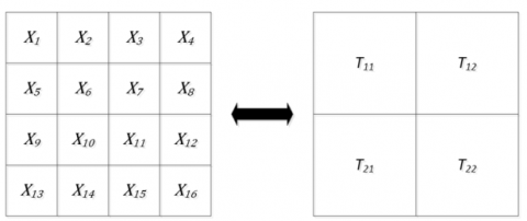
where, $\mathrm{x}_{\mathrm{i} \pm 1, \mathrm{j} \pm 1}$ is the grayscale of the surrounding pixel; $x_{i j}^{R}$ is the mean intensity of region R with xij as the seed point; Th is the given threshold. Formula (15) reveals two deficiencies with the traditional region growing method. Firstly, the object to be merged is merely a pixel, which carries very limited information, as the most basic unit of the image. The lack of information will bias the final result of region merging. To solve the problem, this paper divides the face image $X_{m \times n}$ into multiple non-intersecting sub-images:
$X_{m \times n}=\left[\begin{array}{cccc}x_{11}, x_{12}, & \cdots & x_{1 n} \\ \vdots & \ddots & \vdots \\ x_{m 1}, x_{m 1}, & \cdots & x_{m n}\end{array}\right]=\left[\begin{array}{cccc}T_{11}, T_{12}, & \cdots & T_{1 J} \\ \vdots & \ddots & \vdots \\ T_{I 1}, T_{I 1}, & \cdots & T_{I J}\end{array}\right]$ (16)
Any sub-image $\mathrm{T}_{\mathrm{ij}}(1 \leq \mathrm{i} \leq \mathrm{I}, 1 \leq \mathrm{j} \leq \mathrm{J})$ contains multiple pixels. Hence, the non-intersecting sub-images Tij could carry lots of information of the original image. The division is nondestructive and reversible (Figure 3).
Figure 3. Dividing the original image into multiple sub-images
Secondly, the key of region growing is the definition of growth rule. Due to the natural complexity of face images, the growth rule should be configured in the light of the various attributes of the original image. The traditional growth rule mainly relies on the grayscale difference. However, the grayscale of a single pixel cannot reflect the rich information of the original image. To solve the problem, this paper takes sub-images as the basic unit of region growing. The sub-images retain most of the features of the original image, namely, brightness, contrast, structure, color, texture, and spatial distribution. To further improve the accuracy of region merging with sub-images as the basic unit, this paper puts forward a brand-new growth rule called fusion similarity measurement mechanism (FSMM).
After being converted into a grayscale matrix, the original image becomes meaningful in mathematical calculation. Let X and Y be the grayscale matrices of two adjacent sub-images, respectively (During region growing, sub-image Y can be any of the eight adjacent sub-images of sub-image X), $\mathrm{X}=\left[\begin{array}{ccc}\mathrm{X}_{1} & \cdots & \cdots \\ \cdots & \ddots & \cdots \\ \cdots & \cdots & \mathrm{X}_{\mathrm{c}}\end{array}\right], \mathrm{Y}=\left[\begin{array}{ccc}\mathrm{Y}_{1} & \cdots & \cdots \\ \cdots & \ddots & \cdots \\ \cdots & \cdots & \mathrm{Y}_{\mathrm{c}}\end{array}\right]$. Then, the similarity between X and Y can be measured by Euclidean distance:
$d(X, Y)=\sqrt[2]{\sum_{i=1}^{n}\left(X_{i}-Y_{i}\right)^{2}}$ (17)
Many scholars have adopted Euclidean distance to measure the similarity between two matrices, and to regulate region growing. The measurement can accurately characterize the difference between two sub-images in mathematical properties. This difference is directly exhibited in terms of image colors. However, the similarity rule, which solely considers the mathematical difference between grayscale matrices, cannot fully demonstrate the other properties of the image.
Below is an example illustrating the limitation of Euclidean distance as region growing rule: Suppose there are three grayscale matrices $\mathrm{T}_{1}=\left[\begin{array}{lll}0 & 0 & 0 \\ 0 & 0 & 0 \\ 0 & 0 & 0\end{array}\right], \mathrm{T}_{2}=\left[\begin{array}{ccc}7 & 6 & 3 \\ 15 & 20 & 11 \\ 6 & 3 & 5\end{array}\right]$, and $\mathrm{T}_{3}=\left[\begin{array}{ccc}0 & 0 & 0 \\ 0 & 0 & 0 \\ 0 & 0 & 255\end{array}\right]$. The Euclidean distances between T1 and T2, and T1 and T3 are denoted as θ1 and θ2, respectively. Since θ1<θ2, T1 is more similar to T2. However, after the matrices are converted to grayscale images, T1 is more similar to T3 even in naked eyes. In this example, images T1 and T3 have very similar colors. However, their Euclidean distance (color eigenvalue) is exaggerated by a salient eigenvalue. The mis-judgement is attributed to the fact that Euclidean distance (color eigenvalue) is solely considered to compute the grayscale matrices of the two images. The salient value of T3 could be the result of texture or shape features of the image.
To solve the above problem, the Jaccard similarity index is introduced to compute the similarity θ between the grayscale matrices of the two images. The Jaccard similarity index, a metric of the similarity between two sets, is defined as the number of pixels in the interaction between two sets, divided by the number of pixels in the union of two sets:
$\rho(X, Y)=|X \cap Y| /|X \cup Y|$ (18)
In this paper, the Jaccard similarity index is taken as the optimization value in the result of formula (17):
$\theta=d(X, Y) / \rho(X, Y)+\sigma$ (19)
where, d(X,Y) is the Euclidean distance between the grayscale matrices of two images; ρ(X,Y) is the Jaccard similarity index between the grayscale matrices of two images; σ is a small positive number that prevents the denominator from being zero.
The above-mentioned example can prove that the θ value derived from both Euclidean distance and Jaccard similarity index can largely reflect the similarity between the grayscale matrices of two images, and serve as the growth rule. However, some special cases are found during the experiments, in which the above formula is not applicable. Another example was given to explain the influence of the special cases.
Suppose two local grayscale matrices $\mathrm{T}_{1}=\left[\begin{array}{lll}7 & 9 & 8 \\ 4 & 3 & 7 \\ 1 & 5 & 6\end{array}\right]$, and $\mathrm{T}_{2}=\left[\begin{array}{lll}8 & 7 & 9 \\ 3 & 4 & 7 \\ 6 & 5 & 1\end{array}\right]$ are obtained from the same image. The similarity θ between them, which is calculated by formula (19), is far smaller than the expectation θ' given during the explements. θ^' is a preset threshold. If θ>θ', the grayscale matrices are not similar; otherwise, the grayscale matrices are similar. It can be observed from the experimental values in matrices T1 and T2 that formula (19) cannot calculate the correct θ value, due to its neglection of spatial distribution features of the images. Hamming distance is often employed to measure the difference between two spatial vectors of the same structure and size. This criterion sequentially compares the values in the corresponding positions of two spatial vectors X and Y. If Xi=Yi, value is 0; otherwise, the value is 0. After all the corresponding positions of two spatial vectors have been compared, all the ones will be cumulated to obtain the Hamming distance between the two spatial vectors:
$\mu(X, Y)=\sum_{i=1}^{n} X_{i} \bigoplus Y_{i}$ (20)
In this paper, the values are extracted from each grayscale matrix by formula (1). Thus, the values in the grayscale matrices are approximate. The color information of the images cannot be truthfully reflected, with Hamming distance as the only criterion. What is worse, the Hamming distance cannot be directly applied to formula (19).
To solve these problems, Hamming distance is combined with the result of perceptual hash algorithm into a disturbance φ for formula (19), further improving the correctness of the similarity θ between grayscale matrices. Combining formulas (19) and (20), the similarity θ between the grayscale matrices of two images can be expressed as:
$\theta=\varphi(d(X, Y) / \rho(X, Y)+\sigma)$ (21)
Suppose the two contrastive spatial vectors are grayscale matrices X and Y of face images. Each matrix contains c pixels. Then, the disturbance φ can be calculated by:
$\varphi=\left\{\begin{array}{cc}\theta^{\prime} \times(\rho(X, Y)+\sigma) / d(X, Y), & \mu(X, Y)<0.078 \times c \\ 1, & 0.078 \times c \leq \mu(X, Y) \leq 0.156 \times c \\ 1 / \lg \times(m \times n-\mu(X, Y)), & \mu(X, Y)>0.156 \times c\end{array}\right.$ (22)
where, c is sample size; θ' is a preset threshold.
Structural similarity (SSIM) is a full reference image quality evaluation index. The traditional image quality metrics, such as mean squared error (MSE) and peak signal-to-noise ratio (PSNR), deviate from the actual visual perception of human eyes. By contrast, SSIM considers the visual features of human eyes, and adapts to the visual perception of humans. MSE and PSNR evaluates absolute errors, while SSIM, a perception-based metric, takes account of the fuzzy perceptual changes of image structure. The SSIM includes some phenomena related to perceptual changes, including brightness and contrast. The structural information refers to the internal dependence between pixels, especially the spatially close ones. The dependence carries important information about the visual perception of objects.
The SSIM ranges from 0 to 1. The greater the SSIM, the higher the similarity between two images. Based on the SSIM theory, the structural information is defined from the angle of image composition as an attribute reflecting the object structure in the scene, and independent of brightness and contrast, while distortion is modeled as the combination of brightness, contrast, and structure. Let X and Y be the reference image and the distorted image. Then, the following definitions can be established:
$l\left(T_{i \times j}, T_{(i \pm 1) \times(j \pm 1)} \quad \right)=\left(2 u_{X} u_{Y}+C_{1}\right) /\left(u_{X}^{2}+u_{Y}^{2}+C_{1}\right)$ (23)
$c(X, Y)=\left(2 \sigma_{X} \sigma_{Y}+C_{2}\right) /\left(\sigma_{X}^{2}+\sigma_{Y}^{2}+C_{2}\right)$ (24)
$s(X, Y)=\left(\sigma_{X Y}+C_{3}\right) /\left(\sigma_{X} \sigma_{Y}+C_{3}\right)$ (25)
where, uX and uY are the mean of images X and Y, respectively, reflecting the brightness of each image; σX and σY are the variances of images X and Y, respectively, reflecting the contrast of each image; C1, C2, and C3 are very small positive integers that prevent the denominator from being zero. Based on the above three information, the SSIM can be calculated by:
$\operatorname{SSIM}(X, Y)=[l(X, Y)]^{\alpha} \cdot[c(X, Y)]^{\beta} \cdot[s(X, Y)]^{\gamma}$ (26)
where, $\alpha, \beta$, and $\gamma$ are the weights of different eigenvalues. If $\alpha=\beta=\gamma=1, \mathrm{C}_{1}=\left(\mathrm{K}_{1} \mathrm{~L}\right)^{2}, \mathrm{C}_{2}=\left(\mathrm{K}_{2} \mathrm{~L}\right)^{2}, \mathrm{C}_{3}=\mathrm{C}_{2} / 2$, and $\mathrm{K}_{1} \ll 1, \mathrm{~K}_{2} \ll 1$, with L being the dynamic range of the image, formula (26) can be simplified as:
$\operatorname{SSIM}(X, Y)=\left(2 u_{X} u_{Y}+C_{1}\right)\left(2 \sigma_{X} \sigma_{Y}+C_{2}\right) /\left(u_{X}^{2}+u_{Y}^{2}+C_{1}\right)\left(\sigma_{X}^{2}+\sigma_{Y}^{2}+C_{2}\right)$ (27)
To sum up, the FSMM mechanism can be expressed as:
$\operatorname{FSMM}(X, Y)=\frac{\varphi \times(d(X, Y) / \rho(X, Y)+\sigma) \times\left(2 u_{X} u_{Y}+C_{1}\right) \times\left(2 \sigma_{X} \sigma_{Y}+C_{2}\right)}{\left(u_{X}^{2}+u_{Y}^{2}+C_{1}\right) \times\left(\sigma_{X}^{2}+\sigma_{Y}^{2}+C_{2}\right)}$ (28)
The innovation of RGP algorithm lies in merging similar sub-images into one region via region growing. When RGP and LAP have the same privacy budget, RGP can produce a smaller noise error during privacy protection of images. During image growing, the face image $X_{m \times n}$ is segmented into k sub-images of the same structure. Then, a sub-image Tij is selected randomly as the seed point, and assigned a privacy budget of $\varepsilon / \mathrm{k}$. Then, LAP is called to add a Laplace noise to the produce $\mathrm{T}_{\mathrm{ij}}^{\prime}$. Whether an adjacent $\mathrm{T}_{(\mathrm{i} \pm 1)(\mathrm{j} \pm 1)}$ needs to be merged into the growing region of the current seed point depends on whether the gap between $\mathrm{T}_{\mathrm{ij}}^{\prime}$ and $\mathrm{T}_{(\mathrm{i} \pm 1)(\mathrm{j} \pm 1)}$ satisfies the preset threshold. If $\operatorname{FSMM}\left(\mathrm{T}_{\mathrm{ij}^{\prime}}^{\prime} \mathrm{T}_{(\mathrm{i} \pm 1)(\mathrm{i} \pm 1)}\right) \leq \mathrm{Th}$ (Th is the preset threshold), $\mathrm{T}_{(\mathrm{i} \pm 1)(\mathrm{j} \pm 1)}\quad$ will be replaced with $\mathrm{T}_{\mathrm{ij}}^{\prime}$ before publication. Once no more qualified sub-image can be merged with Tij being the seed point, a new seed point will be selected randomly from the remaining sub-images, and the above process will be repeated until the entire image is fully grown.
Note that no privacy budget is consumed as $\mathrm{T}_{(\mathrm{i} \pm 1)(\mathrm{j} \pm 1)}$ is replaced with $\mathrm{T}_{\mathrm{ij}}^{\prime}$. Hence, the privacy budget assigned to $\mathrm{T}_{(\mathrm{i} \pm 1)(\mathrm{j} \pm 1)}\quad$ will be retained for use in subsequent operations.
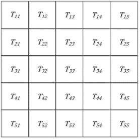
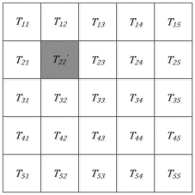
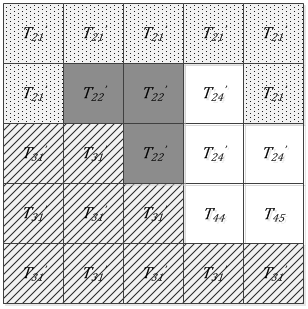
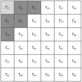
To facilitate understanding, an example was provided to explain the implementation of RGP. The sub-image division is displayed in Figure 4: $\mathrm{X}_{\mathrm{m} \times \mathrm{n}}=\left(\mathrm{T}_{11}, \mathrm{~T}_{12}, \mathrm{~T}_{13}, \ldots, \mathrm{T}_{55}\right)$. Out of the sub-images, a random sub-image is selected as the seed point, and assigned a privacy budget of the size $\varepsilon / 25$. As shown in Figure 5, $\mathrm{T}_{22}^{\prime}$ serves as the seed point, i.e., the disturbance obtained by adding Laplace noise to T22. In this case, the state of T22 is labeled. After the seed point is selected, a chain will be created to temporarily store the seed points and candidate seed points.
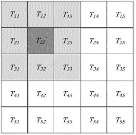
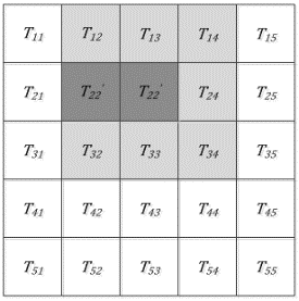
Next, the seed point will be compared with each of the eight adjacent sub-images via region growing (Figure 6). If a sub-image is sufficiently similar and in line with the merging condition, replacement will be carried out, and the sub-image will be added to the temporary chain list as a candidate seed point. As shown in Figure 7, T23 is the only sub-image whose similarity with the seed point satisfies the preset threshold. Hence, T23 is replaced with $\mathrm{T}_{22}^{\prime}$, the current seed point is removed from the chain list, and the candidate seed point is selected as the new seed point. The above process is repeated until the temporary chain list is empty.
Figure 4. Image division
Figure 5. Seed point selection
Figure 6. Traversing adjacent regions
Figure 7. Replacement
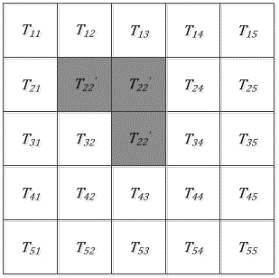
Figure 8. Result of local region growing
Figure 9. Result of global region growing
Figure 8 shows the labeled region after one region growing. A seed is selected from the unlabeled region, and the above steps are repeated, until all sub-images are labeled. Figure 9 shows the noisy grayscale matrix after four region growing operations.
The specific implementation of RGP is summarized as follows:
Algorithm 1: RGP
Inputs: Original image X, privacy budget $\varepsilon$, preset parameters a and b, and expectation for sub-image similarity Th
Output: Image X' satisfying differential privacy
RGP provides a way to protect the privacy of face images based on region growing and differential privacy. Lines 5-7 define two variables and set the termination condition (while circulation). The two variables are z and εleft. The former ensures that, after the algorithm completes, each sub-image T1[i][j] will be converted into a noisy sub-image $\mathrm{T}_{1}^{\prime}[\mathrm{i}][\mathrm{j}]$, while εleft defines the initial value for the allocation of privacy budget ε. Lines 8-18 specifies the seed point selection of region growing. Specifically, Lines 8-11 judge whether T1[i][j] has been merged to a region. If it has been labeled, it is necessary to choose a new seed point. Lines 12-17 release the labeled seed point from the chain list, and select the next seed point from the candidates. Line 18 changes the state of the current seed point from unlabeled to labeled. Lines 19-21 assign a proper privacy budget and add a noise to the current seed point. Line 22 saves the current seed point to the chain list. Lines 23-25 demand that the adjacent region T1[m][n] of the seed point should not surpass the image boundary and the labeled state. Lines 26-28 use the FSMM mechanism to compute the similarity between an adjacent region and the seed point, and judge if the former meets the growth rule. If yes, T1[m][n] will be replaced with $\mathrm{T}_{1}^{\prime}[\mathrm{i}][\mathrm{j}]$. Lines 29-34 judge whether T1[m][n] that satisfies growth rule exists in the chain list. If not, this region will be added to the chain list, and become a candidate seed point.
Note that Lines 19-21 of RGP provide a dynamic allocation (DA) mechanism for privacy budget. Unlike the common binary allocation mechanism, DA offers a more reasonable solution to the privacy budget allocation during region growing, and reduces the influence of noise on the original data. The DA mechanism can be described as follows:
Suppose each region growing consumes a privacy budget of εi={ε1,ε2,ε3,…,εm }, each merged region contains si={s1,s2,s3,…,sm} sub-images, and s1+s2+s3+⋯+sm=k,with k=a×b being the total number of sub-images. Let $\varepsilon_{\mathrm{i}}^{\mathrm{left}}$ be the residual privacy budget after the completion of state i. Then, the $\varepsilon_{\mathrm{i}}$ and $\varepsilon_{\mathrm{ileft}}$ in any state under the DA mechanism can be expressed as:
$\varepsilon_{i}=\varepsilon_{i-1}^{l e f t} /\left(k-\sum_{j=1}^{i-1} s_{j}\right)$ (29)
$\varepsilon_{i}^{l e f t}=\varepsilon_{i-1}^{l e f t}-\varepsilon_{i}$ (30)
Theorem 3. In RGP, the consumption of privacy budget will not surpass ε, i.e., $\varepsilon_{1}+\varepsilon_{2}+\varepsilon_{3}+\cdots+\varepsilon_{\mathrm{m}} \leq \varepsilon$.
Proof: Formula (29) shows that, when $\mathrm{k}-\sum_{\mathrm{j}=1}^{\mathrm{m}-1} \mathrm{~s}_{\mathrm{j}}=1, \varepsilon_{\mathrm{m}-1 \mathrm{left}}=\varepsilon_{\mathrm{m}} .$ Then, $\varepsilon_{\mathrm{mleft}}=0$. In this case, we have:
$\varepsilon_{1}+\varepsilon_{2}+\varepsilon_{3}+\cdots+\varepsilon_{m}=\varepsilon$
When $\mathrm{k}-\sum_{\mathrm{j}=1}^{\mathrm{m}-1} \mathrm{~s}_{\mathrm{j}}>1, \quad \varepsilon_{\mathrm{m}-\mathrm{1left}} / \varepsilon_{\mathrm{m}}>1$. Then, $\varepsilon_{\mathrm{mleft}}>0$, In this case, we have:
$\varepsilon_{1}+\varepsilon_{2}+\varepsilon_{3}+\cdots+\varepsilon_{m}<\varepsilon$
Q.E.D.
Theorem 4. RGP satisfies ε- differential privacy.
Proof: According to Theorem 3:
$\varepsilon_{1}+\varepsilon_{2}+\varepsilon_{3}+\cdots+\varepsilon_{m} \leq \varepsilon$
where, $\varepsilon_{\mathrm{i}}(1 \leq \mathrm{i} \leq \mathrm{m})$ is the privacy budget consumed under each state. According to the differential privacy-parallel combination property (Property 2), RGP satisfies $\varepsilon$- differential privacy.
Q.E.D.
Theorem 5. The error generated by RGP is no greater than that generated by LAP, i.e.:
Error $(R G P) \leq$ Error $(L A P)$
Proof: The DA mechanism of RGP consumes a privacy budget of $\varepsilon_{\mathrm{i}}=\left\{\varepsilon_{1}, \varepsilon_{2}, \varepsilon_{3}, \ldots, \varepsilon_{\mathrm{m}}\right\}$ each time. The number of submatrices affected by $\varepsilon_{\mathrm{i}}=\left\{\varepsilon_{1}, \varepsilon_{2}, \varepsilon_{3}, \ldots, \varepsilon_{\mathrm{m}}\right\}$ can be described by $\mathrm{s}_{\mathrm{i}}=\left\{\mathrm{s}_{1}, \mathrm{~s}_{2}, \mathrm{~s}_{3}, \ldots, \mathrm{s}_{\mathrm{m}}\right\}, \mathrm{s}_{1}+\mathrm{s}_{2}+\mathrm{s}_{3}+\cdots+\mathrm{s}_{\mathrm{m}}=\mathrm{k}$. The Laplace mechanism of LAP consumes a privacy budget of $\varepsilon / \mathrm{k}, \sum_{\mathrm{i}=1}^{\mathrm{k}} \mathrm{s}_{\mathrm{i}}^{\prime}=\mathrm{k}\left(\mathrm{s}_{1}^{\prime}=\mathrm{s}_{2}^{\prime}=\mathrm{s}_{3}^{\prime}=\cdots=\mathrm{s}_{\mathrm{k}}^{\prime}=1\right)$ each time.
Firstly, the maximum possible error of DA mechanism is calculated, revealing that $\mathrm{s}_{1}=\mathrm{s}_{2}=\mathrm{s}_{3}=\cdots \mathrm{s}_{\mathrm{m}}=1$, i.e., m=k. Thus, we have:
$\operatorname{Error}(R G P)_{\max }=\left(\operatorname{lap}\left(\Delta Q / \varepsilon_{1}\right)+\operatorname{lap}\left(\Delta Q / \varepsilon_{2}\right)+\operatorname{lap}\left(\Delta Q / \varepsilon_{3}\right)+\right.$
$\left.\cdots \operatorname{lap}\left(\Delta Q / \varepsilon_{m}\right)\right)_{\max }=\sum_{i=1}^{k} \operatorname{lap}\left(\Delta Q / \varepsilon_{i}\right)=k \times \operatorname{lap}(\Delta Q /$
$(\varepsilon / k))=\operatorname{Error}(L A P)$
The other situations can be judged by formula (30). After the completion of state i, the residual privacy budget of DA mechanism is εileft, while that of Laplace mechanism is $\varepsilon_{\text {ileft }}^{\prime}$. Since DA mechanism allows an si>1, and $\mathrm{s}_{1}=\mathrm{s}_{2}=\mathrm{s}_{3}=\cdots \mathrm{s}_{\mathrm{i}-1}=1(1<\mathrm{i}<\mathrm{m})$, we have:
$\varepsilon_{\text {ileft }}-\varepsilon_{\text {ileft }}^{\prime}=\left(\varepsilon-\varepsilon \times \frac{k-\left(i-1+s_{i}\right)}{k}\right)-\left(\varepsilon-\varepsilon \times \frac{k-i}{k}\right)=\varepsilon \times$
$\left(\frac{k-i}{k}-\frac{k-\left(i-1+s_{i}\right)}{k}\right)=\varepsilon \times \frac{s_{i}-1}{k}$
Since $s_{i}>1 \quad, \quad \varepsilon_{\text {ileft }}-\varepsilon_{\text {ileft }}^{\prime}>0$. Thus, $\left(\varepsilon_{i+1}, \varepsilon_{i+2}, \varepsilon_{i+3}, \ldots, \varepsilon_{m}\right)>\varepsilon / k$. It can be seen that Error(RGP)<Error(LAP).
Q.E.D.
3.3 Atypical region growing publication (ARGP)
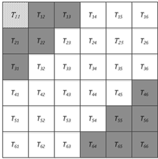
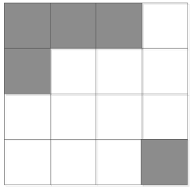
If the RGP is applied to an image, the merged region through one region growing with T11 as the seed point can be illustrated in Figure 10 (the dark region). From the perspective of the entire image, i.e., removing the limitation on region growing direction, the similarity θ between $\mathrm{T}_{11}^{\prime}$ and each unlabeled sub-image is calculated, and all the qualified sub-images are merged together. But the merged region may not be as expected (Figure 11). Obviously, the current merged region is not continuous in 2D space (RGP cannot yield such a merged region), but every sub-image of the merged region satisfies θ<=Th.
Figure 10. Region growing direction estimated by RGP
To find more qualified sub-images for the seed point without damaging ε-differential privacy, this paper integrates atypical region growing with differential privacy into a novel privacy protection approach for image publication, denoted as ARGP. Different from traditional region growth strategy, the ARGP does not restrict the growing direction within adjacent sub-images, but searches for qualified sub-images among all unlabeled sub-images, using the exponential mechanism. The specific steps of the ARGP are as follows:
Algorithm 2. ARGP
Inputs: Original image X, privacy budget ε, preset parameters a and b, and expectation for sub-image similarity Th
Output: Image X' satisfying differential privacy
In ARGP, Line 4 divides the privacy budget ε into two parts: a part ε1 for exponential mechanism, and a part ε2 for noise addition. Lines 5-7 define two variables and set the termination condition (while circulation). The two variables are w and εleft. The former ensures that, after the algorithm completes, each sub-image T1[i][j] will be converted into a noisy sub-image $\mathrm{T}_{1}^{\prime}[\mathrm{i}][\mathrm{j}]$, while εleft defines the initial value for the allocation of privacy budget ε. Lines 8-14 specifies that, if there is no seed point, an unlabeled sub-image will be selected randomly as the seed point; then, the seed point will be labeled, and added a noise by DA mechanism. Lines 15-16 realize the RGP. Lines 17-20 select a sub-image by the exponential mechanism. Specifically, Line 17 defines the scoring function of exponential mechanism. ARGP intends to select the sub-image more similar to the seed point at a larger probability. Σ is a very small positive number that prevents the denominator from being zero. In Line 18, Δu is the sensitivity of the scoring function. Since adding/removing one record only affects one count of θ, Δu=1. Lines 21-28 use the FSMM mechanism to compute the similarity between the seed point and the selected T1[m][n]. If the result satisfies the preset threshold, assign the value of $\mathrm{T}_{1}^{\prime}[\mathrm{i}][\mathrm{j}]$ to T1[m][n], and set it as the new seed point. Otherwise, select a new seed point, and repeat the above process until all sub-images become noisy.
For ARGP, the exponential mechanism does not necessarily lead to the needed optimal solution, but capable of obtaining the optimal or near optimal solution at a high probability. Table 1 shows the test results on the selection probability of the exponential mechanism in ARGP. The test aims to select the minimum of a set of random numbers. Column 1 reports the similarity θ between the seed point and sub-regions. Column 2 reports the scoring function (σ=0.02). The other four columns report the section probabilities of each sub-region at different ε values, and the sum of each column equals or approximates 1 (the error induced by indivisibility). If ε=0, the level of privacy protection is maximized, and all sub-regions are selected at the same probability. With the growth of ε, the selection probability increases with the value of the scoring function ΔQ; the inverse is also true.
Figure 11. Region growing direction estimated by ARGP
Table 1. Exponential mechanism- minimum selection probability test
|
$\theta$ |
$\Delta \mathrm{Q}$ |
$\varepsilon$=0 |
$\varepsilon$=0.05 |
$\varepsilon$=0.1 |
$\varepsilon$=0.5 |
|
15 |
0.0666 |
14.29% |
2.15% |
0.21% |
0.20% |
|
62 |
0.0161 |
14.29% |
0.73% |
0.00% |
0.00% |
|
28 |
0.0357 |
14.29% |
1.01% |
0.10% |
0.00% |
|
7 |
0.1425 |
14.29% |
14.50% |
6.12% |
0.52% |
|
8 |
0.1247 |
14.29% |
13.21% |
6.19% |
0.51% |
|
1 |
0.9804 |
14.29% |
67.56% |
87.32% |
98.77% |
|
37 |
0.0270 |
14.29% |
0.86% |
0.06% |
0.00% |
Theorem 6. ARGP satisfies ε-differential privacy.
Proof: ARGP divides the privacy budget ε into two parts: ε=ε1+ε2, where ε1 is used to select unlabeled sub-region T by the exponential mechanism; the selection probability is positively correlated with exp $\left(\frac{\varepsilon_{1} \Delta Q}{2 \Delta u}\right)$:
$\operatorname{Pr}[\mathrm{M}(\mathrm{X}, \Delta \mathrm{Q})=\mathrm{T}]=\frac{\exp \left(\frac{\varepsilon_{1} \Delta \mathrm{Q}(\mathrm{X}, \mathrm{T})}{2 \Delta \mathrm{u}}\right)}{\sum_{\mathrm{T}^{\prime} \in O} \exp \left(\frac{\varepsilon_{1} \Delta \mathrm{Q}\left(\mathrm{X}, \mathrm{T}^{\prime}\right)}{2 \Delta \mathrm{u}}\right)}$ (31)
For the given X and its adjacent region X', the following can be derived from formula (31) for any $\mathrm{T} \in \mathrm{O}$:
$\frac{\operatorname{Pr}[M(X, \Delta Q)=T]}{\operatorname{Pr}\left[M\left(X^{\prime}, \Delta Q\right)=T\right]}=\frac{\frac{\exp \left(\frac{\varepsilon_{1} \Delta Q(X, T)}{2 \Delta u}\right)}{\sum_{T^{\prime} \in O} \exp \left(\frac{\varepsilon_{1} \Delta Q\left(X, T^{\prime}\right)}{2 \Delta u}\right)}}{\frac{\exp \left(\frac{\varepsilon_{1} \Delta Q\left(X^{\prime}, T\right)}{2 \Delta u}\right)}{\sum_{T^{\prime} \in O} \exp \left(\frac{\varepsilon_{1} \Delta Q\left(X^{\prime}, T^{\prime}\right)}{2 \Delta u}\right)}}$
$=\left(\frac{\exp \left(\frac{\varepsilon_{1} \Delta Q(X, T)}{2 \Delta u}\right)}{\exp \left(\frac{\varepsilon_{1} \Delta Q\left(X^{\prime}, T\right)}{2 \Delta u}\right)}\right) \times\left(\frac{\sum_{T^{\prime} \in O} \exp \left(\frac{\varepsilon_{1} \Delta Q\left(X^{\prime}, T^{\prime}\right)}{2 \Delta u}\right)}{\sum_{T^{\prime} \in O} \exp \left(\frac{\varepsilon_{1} \Delta Q\left(X, T^{\prime}\right)}{2 \Delta u}\right)}\right)$
$=\exp \left(\frac{\varepsilon_{1}\left(\varepsilon_{1} \Delta Q(X, T)-\varepsilon_{1} \Delta Q\left(X^{\prime}, T\right)\right)}{2 \Delta u}\right) \times\left(\frac{\sum_{T^{\prime} \in o} \exp \left(\frac{\varepsilon_{1} \Delta Q\left(X^{\prime}, T^{\prime}\right)}{2 \Delta u}\right)}{\sum_{T^{\prime} \in o} \exp \left(\frac{\varepsilon_{1} \Delta Q\left(X, T^{\prime}\right)}{2 \Delta u}\right)}\right)$
$\leq \exp \left(\frac{\varepsilon_{1}}{2}\right) \times\left(\frac{\sum_{T^{\prime} \in O} \exp \left(\frac{\varepsilon_{1}}{2}\right) \times \exp \left(\frac{\varepsilon_{1} \Delta Q\left(X, T^{\prime}\right)}{2 \Delta u}\right)}{\sum_{T^{\prime} \in O} \exp \left(\frac{\varepsilon_{1} \Delta Q\left(X, T^{\prime}\right)}{2 \Delta u}\right)}\right)$
$\leq \exp \left(\frac{\varepsilon_{1}}{2}\right) \times \exp \left(\frac{\varepsilon_{1}}{2}\right) \times\left(\frac{\sum_{T^{\prime} \in O} \exp \left(\frac{\varepsilon_{1} \Delta Q\left(X, T^{\prime}\right)}{2 \Delta u}\right)}{\sum_{T^{\prime} \in O} \exp \left(\frac{\varepsilon_{1} \Delta Q\left(X, T^{\prime}\right)}{2 \Delta u}\right)}\right)=\exp \left(\varepsilon_{1}\right)$
Hence, the exponential-based selection of unlabeled sub-region of ARGP satisfies ε1-differential privacy. From the proof of Theorem 4, it can be learned that the noise addition of ARGP satisfies ε2-differential privacy. Overall, ARGP satisfies ε-differential privacy in the whole process.
Q.E.D.
Theorem 7. When an image is divided on equal conditions, the number zj of sub-images to be merged to a seed point in ARGP must be greater than or equal to the number s_i of sub-images to be merged to the same seed point in RGP, under ideal conditions, that is, Error(ARGP)≤Error(RGP).
Proof: Theorem 7 can be proved by contradiction. It is assumed that zj<si.
In ARGP, there exists a sub-image T0, whose merged region is set A, i.e., $\mathrm{T}_{0} \in \mathrm{A}$, with zj being the number of elements in set A. In RGP, the merged region of the same sub-image T0 is set B, i.e., $\mathrm{T}_{0} \in \mathrm{B}$, with si being the number of elements in set B. If zj<si holds, then there must exist a sub-image Tx satisfying Tx∉A in ARGP and Tx∈B in RGP.
From the growing direction and seed point selection of the two algorithms, if Tx∈B, then there must exist Tx∈A. Thus, zj<si is invalid.
Q.E.D.
Figure 12. zj=si
The conclusion of Theorem 7 can be further analyzed by dividing zj≥si into zj=si and zj>si. Suppose there is an image will produce δ merged regions by RGP or ARGP (Figure 12; the merged regions are in dark color). If the exponential mechanism cannot obtain the qualified sub-images for merging, then any zj=si. From the proof of Theorem 5, we have:
$\left\{\begin{array}{rlc}\text { Error }(A R G P)\max=\operatorname{Error}(R G P)_{\max }=\operatorname{Error}(\mathrm{Lap}), & \delta=0 \\ \operatorname{Error}(A R G P)=\operatorname{Error}(R G P)<\operatorname{Error}(\operatorname{Lap}), & 1 \leq \delta \leq k / 2 \text { or }-1 \leq \delta \leq\left(a^{*} b\right) / 2\end{array}\right.$
As shown in Figure 13, if the exponential mechanism can obtain any qualified sub-images, which are not connected with the current merged region, then zj>si. It can be derived from formula (30) that:
$\varepsilon_{R G P l e f t}-\varepsilon_{A R G P l e f t}=\left(\varepsilon-\varepsilon \times \frac{k-\left(\gamma-1+s_{i}\right)}{k}\right)-\left(\varepsilon-\varepsilon \times \frac{a * b-\left(\gamma-1+z_{j}\right)}{a * b}\right)==\varepsilon *$
$\left(\frac{a * b-\left(\gamma-1+z_{j}\right)}{a * b}-\frac{k-\left(\gamma-1+s_{i}\right)}{k}\right)=\varepsilon \times \frac{s_{i}-z_{j}}{k}$
Since zj>si, εRGPleft-εARGPleft<0. Thus, Error(ARGP)<Error(RGP).
Q.E.D.
Figure 13. zj>si
4.1 Experiments
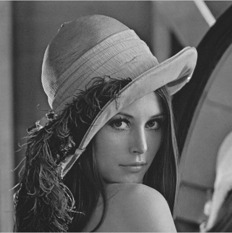
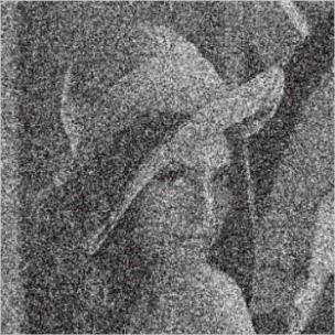
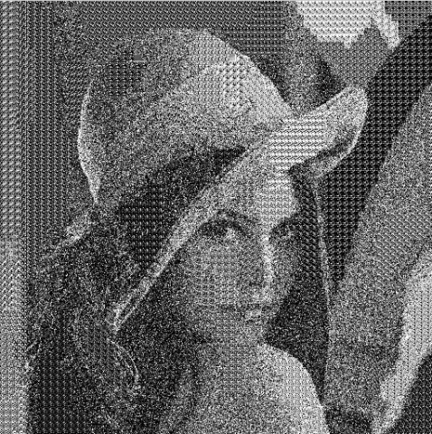
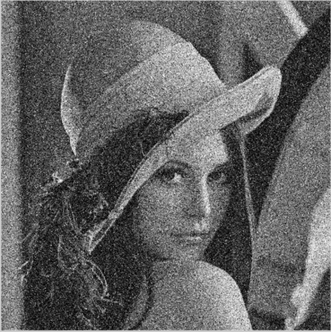
Among the various kinds of images, face images have the most representative sensitivity information. To verify its feasibility, our algorithm was tested on LENA.JPG (size: 512*512). During the execution of the algorithm, the original image was split into 4,096 sub-images of the size 8*8. The following figures present the test results of different algorithms under the same conditions: Figure 14 shows the original image; Figure 15 shows the results of direct addition of Laplace noise to the original image; Figure 16 shows the result obtained by RGP; Figure 17 shows the result obtained by ARGP. Apparently, Figures 16 and 17 are closer to the original image than Figure 15, and the result of ARGP is better than that of LPA and RGP.
Figure 14. Original image
Figure 15. Result of LAP
Figure 16. Result of RGP
Figure 17. Result of ARGP
Now, a preliminary conclusion can be drawn: RGP and ARGP are superior to LAP. But the conclusion is merely obtained by observing the images on test results. It might be one-sided or inaccurate. To further validate the conclusion, the four images were converted into grayscale histograms and compared once more. Grayscale histogram demonstrates the relationship between the occurrence frequency of pixels on each grayscale and grayscale. Although it does not reflect the specific distribution of image pixels, the grayscale histogram statistically showcases the similarity between different images.
Figure 18. Grayscale histogram of the original image
Figure 19. Grayscale histogram of LAP result
Figure 20. Grayscale histogram of RGP result
Figure 21. Grayscale histogram of ARGP result
As shown in Figures 18-21, under the same conditions, the histogram of RGP has similar distribution as that of LAP, but differs significantly from that of the original image. The pixel distribution of ARGP’s histogram is basically the same as that of the original image. Hence, ARGP has the least noise disturbance to the image, and achieves the highest availability.
4.2 Result analysis
Table 2. ORL & Precision
|
Precision |
LAP |
SWP |
RGP |
Sort-SWP |
ARGP |
|
ε=1 |
6.5% |
39.3% |
47.4% |
53.9% |
54.6% |
|
ε=ln7 |
8.7% |
42.4% |
56.5% |
69.0% |
72.3% |
|
ε=ln20 |
11.4% |
47.3% |
63.6 % |
71.9% |
73.2% |
|
ε=5 |
16.7% |
62.7% |
70.1% |
82.8% |
83.6% |
|
ε=10 |
18.6% |
68.7% |
73.6% |
85.1% |
85.7% |
Table 3. ORL & Recall
|
Recall |
LAP |
SWP |
RGP |
Sort-SWP |
ARGP |
|
ε=1 |
71.3% |
78.0% |
80.6% |
83.6% |
82.7% |
|
ε=ln7 |
73.2% |
75.0% |
81.7% |
81.2% |
83.1% |
|
ε=ln20 |
74.7% |
83.8% |
82.1% |
84.0% |
83.9% |
|
ε=5 |
77.9% |
76.3% |
84.6% |
86.1% |
88.0% |
|
ε=10 |
80.1% |
82.2% |
86.6% |
88.1% |
88.3% |
Table 4. ORL & F1-score
|
F1-score |
LAP |
SWP |
RGP |
Sort-SWP |
ARGP |
|
ε=1 |
11.9% |
52.3% |
59.7% |
65.5% |
65.8% |
|
ε=ln7 |
15.5% |
54.2% |
66.8% |
74.6% |
77.3% |
|
ε=ln20 |
19.8% |
60.5% |
71.7% |
77.5% |
78.2% |
|
ε=5 |
27.5% |
68.8% |
76.7% |
84.4% |
85.7% |
|
ε=10 |
30.2% |
74.8% |
79.6% |
86.6% |
87.0% |
Table 5. YALE & Precision
|
Precision |
LAP |
SWP |
RGP |
Sort-SWP |
ARGP |
|
ε=1 |
4.1% |
27.3% |
33.2% |
44.5% |
55.3% |
|
ε=ln7 |
6.5% |
31.1% |
37.8% |
56.3% |
60.2% |
|
ε=ln20 |
9.6% |
39.0% |
45.2% |
62.7% |
66.9% |
|
ε=5 |
13.0% |
59.3% |
60.1% |
75.9% |
77.3% |
|
ε=5 |
18.6% |
63.5% |
68.5% |
77.4% |
78.9% |
Table 6. YALE & Recall
|
Recall |
LAP |
SWP |
RGP |
Sort-SWP |
ARGP |
|
ε=1 |
77.3% |
77.5% |
77.4% |
84.2% |
84.0% |
|
ε=ln7 |
77.6% |
77.7% |
79.1% |
81.7% |
83.1% |
|
ε=ln20 |
79. 4% |
82.6% |
85.8% |
86.8% |
87.5% |
|
ε=5 |
75.4% |
82.4% |
86.2% |
85.7% |
88.0% |
|
ε=10 |
77.3% |
85.2% |
88.7% |
89.2% |
90.0% |
Table 7. YALE & F1-score
|
F1-sroce |
LAP |
SWP |
RGP |
Sort-SWP |
ARGP |
|
ε=1 |
7.8% |
40.4% |
46.5% |
58.2% |
66.7% |
|
ε=ln7 |
12.0% |
44.4% |
51.2% |
67.7 % |
69.8% |
|
ε=ln20 |
17.1% |
53.0% |
59.2% |
72.8% |
75.8% |
|
ε=4 |
19.6% |
59.3% |
67.0% |
75.6% |
78.9% |
|
ε=10 |
30.0% |
72.8% |
77.3% |
82.9% |
84.1% |
Table 8. IMM & Precision
|
Precision |
LAP |
SWP |
RGP |
Sort-SWP |
ARGP |
|
ε=1 |
3.9% |
45.6% |
50.1% |
62.6% |
65.4% |
|
ε=ln7 |
6.5% |
51.2% |
63.2% |
72.3% |
76.5% |
|
ε=ln20 |
8.6% |
57.8% |
69.1% |
75.3% |
82.1% |
|
ε=5 |
10.7% |
68.6% |
75.8% |
84.0% |
87.5% |
|
ε=10 |
15.2% |
75.6% |
79.6% |
88.9% |
91.2% |
Table 9. IMM & Recall
|
Recall |
LAP |
SWP |
RGP |
Sort-SWP |
ARGP |
|
ε=1 |
54.6% |
81.2% |
83.7% |
84.1% |
85.6% |
|
ε=ln7 |
58.2% |
80.7% |
82.7% |
84.5% |
85.9% |
|
ε=ln20 |
63.8% |
85.4% |
86.3% |
88.7% |
89.0% |
|
ε=5 |
66.7% |
78.9% |
83.6% |
87.8% |
90.1% |
|
ε=10 |
70.1% |
83.2% |
85.9% |
88.0% |
91.2% |
Table 10. IMM & F1-score
|
F1-sroce |
LAP |
SWP |
RGP |
Sort-SWP |
ARGP |
|
ε=1 |
7.3% |
58.4% |
62.7% |
71.8% |
74.1% |
|
ε=ln7 |
11.7% |
62.7% |
71.6% |
78.0% |
80.9% |
|
ε=ln20 |
15.2% |
68.9% |
76.7% |
81.5% |
85.4% |
|
ε=5 |
18.4% |
73.4% |
79.5% |
85.9% |
88.8% |
|
ε=10 |
25.0% |
79.2% |
82.6% |
88.4% |
91.2% |
To verify the feasibility of our algorithm, experiments were carried out on ORL, YALE, and IMM face databases, under the environment of Intel® Core i9-9900K CPU @ 3.60 GHz, 32G memory, GTX 21080TI GPU, and Windows 10 operating system. During the experiments, a facial recognition method based on improved AlexNet, a convolutional neural network (CNN), was adopted. This approach has a simpler structure and fewer parameters than AlexNet, and thus saves lots of training time, laying the basis for rapid prediction. The sub-image size was set to 4*4 for the experiment on ORL database, 5*5 for that on YALE database, and 8*8 for that on IMM database. The privacy budget ε was set to 1, ln7, ln20, 5, and 10, respectively. The test metrics are precision, recall, and F1-score. The test results are listed in Tables 2-10.
For differential privacy, the noise level is an important metric of algorithm performance. Under the same conditions, fewer noise means higher feasibility. Of course, noise level is only one of the indices of images, a special information carrier. Our algorithm needs to divide the original image into multiple sub-images before subsequent computing. The sub-image size affects the division results, which in turn influence the total noise generated by the algorithm. In addition to LAP, RGP, and ARGP, XXX’s sliding window publication (SWP) algorithm [1] and sort-SWP algorithm are compared in our experiments. Note that SWP and sort-SWP are realized based on 1D data flows. During image division, the two algorithms can only compute 1D sub-images.
The image size varies between face image databases: 92*112 in ORL, 100*100 in YALE, and 480*640 in IMM. The image division on each database must respect the size of original images. Thus, it is impossible to unify the sub-image size across the databases. The experimental results are displayed in Figures 22-24.
Figure 22. Influence of ORL & sub-image size on noise
Figure 23. Influence of YALE & sub-image size on noise
Figure 24. Influence of IMM & sub-image size on noise
Experimental results show that the total noise generated by an algorithm change with the sub-image size. When the sub-images are too large or too small, the images after privacy protection will have a low availability. The optimal sub-image size is 4*4 for ORL, 5*5 for YALE, and 8*8 for IMM. Thus, it can be derived that the optimal sub-image size is related to the size of the original image. Drawing on the results in Tables 2-10 and Figures 22-24, it was found that image quality affects the final operation results of the algorithms. The better the image quality, the more in line the results are with our expectation.
To solve the privacy protection of face image publication, this paper combines regional growing technique with the Laplace mechanism of differential privacy to add noise to the original image, thereby protecting the sensitive information in face images. Compared with the LAP algorithm, which directly adds Laplace noise to the image, RGP and ARGP can effectively reduce the influence of noise on the protected image, and improve the feasibility of privacy protection on images. Moreover, this paper presents a novel region growing rule: FSMM, and discusses the influence of sub-image size on algorithm results. These conclusions provide an effective reference for other researchers.
It is worth noting that our differential privacy protection approach for face image publication is realized by global noise addition. However, the sensitive information of a face image mostly exists in specific regions (e.g., facial contours, eyes, eyebrows, mouth, and noise). The future work will try to pinpoint the locations of sensitive information, and add noise to these places, aiming to further reduce the noise influence, and enhance the availability of face images after privacy protection.
This work is supported by National Natural Science Foundation of China (Grant No.: 61672179), Natural Science Foundation, Heilongjiang Province, China (Grant No.: LH2021D022, 2019F004), and Fundamental Research Funds, Heilongjiang Provincial Education Department, China (Grant No.: 135309457).
[1] Liu, C., Yang, J., Zhao, W., Zhang, Y., Li, J., Mu, C. (2021). Face image publication based on differential privacy. Wireless Communications and Mobile Computing, 2021(9): 1-20. https://doi.org/10.1155/2021/6680701
[2] Fung, B.C., Wang, K., Philip, S.Y. (2007). Anonymizing classification data for privacy preservation. IEEE Transactions on Knowledge and Data Engineering, 19(5): 711-725. https://doi.org/10.1109/TKDE.2007.1015
[3] Xiao, X., Tao, Y. (2006). Anatomy: Simple and effective privacy preservation. In Proceedings of the 32nd International Conference on Very Large Data Bases, pp. 139-150.
[4] Li, T., Li, N., Zhang, J., Molloy, I. (2010). Slicing: A new approach for privacy preserving data publishing. IEEE Transactions on Knowledge and Data Engineering, 24(3): 561-574. https://doi.org/10.1109/TKDE.2010.236
[5] Terrovitis, M., Liagouris, J., Mamoulis, N., Skiadopoulos, S. (2012). Privacy preservation by disassociation. Proceedings of the VLDB Endowment, 5: 944-955. https://doi.org/10.14778/2336664.2336668
[6] Sweeney, L. (2002). K-anonymity: A model for protecting privacy. International Journal of Uncertainty, Fuzziness and Knowledge-Based Systems, 10(5): 557-570. https://doi.org/10.1142/S0218488502001648
[7] Dwork, C. (2006). Differential privacy. In International Colloquium on Automata, Languages, and Programming. Springer, Berlin, Heidelberg, 1-12. https://doi.org/10.1007/11787006_1
[8] Dwork, C. (2008). Differential privacy: A survey of results. In International Conference on Theory and Applications of Models of Computation. Springer, Berlin, Heidelberg, pp. 1-19. https://doi.org/10.1007/978-3-540-79228-4_1
[9] Dwork, C. (2009). The differential privacy frontier. In Theory of Cryptography Conference, Springer, Berlin, Heidelberg, 496-502. https://doi.org/10.1007/978-3-642-00457-5_36
[10] Dwork, C., Lei, J. (2009). Differential privacy and robust statistics. In Proceedings of the forty-first annual ACM symposium on Theory of computing, Bethesda, MD, USA, pp. 371-380. https://doi.org/10.1145/1536414.1536466
[11] Dwork, C. (2010). Differential privacy in new settings. In Proceedings of the twenty-first annual ACM-SIAM symposium on Discrete Algorithms, Society for Industrial and Applied Mathematics, pp. 174-183. https://doi.org/10.1137/1.9781611973075.16
[12] Dwork, C. (2011). The promise of differential privacy a tutorial on algorithmic techniques. In 2011 IEEE 52nd Annual Symposium on Foundations of Computer Science, pp. 1-2. https://doi.org/10.1109/FOCS.2011.88
[13] Dwork, C., McSherry, F., Nissim, K., Smith, A. (2006). Calibrating noise to sensitivity in private data analysis. In Theory of Cryptography Conference, Springer, Berlin, Heidelberg, pp. 265-284. https://doi.org/10.1007/11681878_14
[14] McSherry, F., Talwar, K. (2007). Mechanism design via differential privacy. In 48th Annual IEEE Symposium on Foundations of Computer Science (FOCS'07), pp. 94-103. https://doi.org/10.1109/FOCS.2007.66
[15] McSherry F. (2010). Privacy integrated queries: An extensible platform for privacy-preserving data analysis. Communications of the ACM, 53(9): 89-97. https://doi.org/10.1145/1810891.1810916
[16] Roth, A., Roughgarden, T. (2010). Interactive privacy via the median mechanism. In Proceedings of the Forty-Second ACM Symposium on Theory of Computing, pp. 765-774. https://doi.org/10.1145/1806689.1806794
[17] Hardt, M., Rothblum, G.N. (2010). A multiplicative weights mechanism for privacy-preserving data analysis. In 2010 IEEE 51st Annual Symposium on Foundations of Computer Science, pp. 61-70. https://doi.org/10.1109/FOCS.2010.85
[18] Gupta, A., Roth, A., Ullman, J. (2012). Iterative constructions and private data release. In Theory of Cryptography Conference, Springer, Berlin, Heidelberg, pp. 339-356. https://doi.org/10.1007/978-3-642-28914-9_19
[19] Fan, L., Xiong, L. (2012). Real-time aggregate monitoring with differential privacy. In Proceedings of the 21st ACM International Conference on Information and Knowledge Management, pp. 2169-2173. https://doi.org/10.1145/2396761.2398595
[20] Kellaris, G., Papadopoulos, S., Xiao, X., Papadias, D. (2014). Differentially private event sequences over infinite streams. Proceedings of the VLDB Endowment, 7(12): 1155-1166. https://doi.org/10.14778/2732977.2732989
[21] Xiao, X., Wang, G., Gehrke, J. (2010). Differential privacy via wavelet transforms. IEEE Transactions on Knowledge and Data Engineering, 23(8): 1200-1214. https://doi.org/10.1109/TKDE.2010.247
[22] Xu, J., Zhang, Z., Xiao, X., Yang, Y., Yu, G., Winslett, M. (2013). Differentially private histogram publication. The VLDB Journal, 22(6): 797-822. https://doi.org/10.1007/s00778-013-0309-y
[23] Li, C., Miklau, G., Hay, M., McGregor, A., Rastogi, V. (2015). The matrix mechanism: optimizing linear counting queries under differential privacy. The VLDB Journal, 24(6): 757-781. https://doi.org/10.1007/s00778-015-0398-x
[24] Li, C., Hay, M., Miklau, G., Wang, Y. (2014). A data-and workload-aware algorithm for range queries under differential privacy. Proceedings of the VLDB Endowment, 7(5): 341-352. https://doi.org/10.14778/2732269.2732271
[25] Zhang, X.J., Fu, C.C., Meng, X.F. (2018). Facial image publication with differential privacy. Journal of Image and Graphics, 23(9): 1305-1315.
[26] Nissim, K., Raskhodnikova, S., Smith, A. (2007). Smooth sensitivity and sampling in private data analysis. In Proceedings of the Thirty-Ninth Annual ACM Symposium on Theory of Computing, pp. 5-84. https://doi.org/10.1145/1250790.1250803
[27] Adams, R., Bischof, L. (1994). Seeded region growing. IEEE Transactions on Pattern Analysis and Machine Intelligence, 16(6): 641-647. https://doi.org/10.1109/34.295913
[28] Matalas, L., Benjamin, R., Kitney, R. (1997). An edge detection technique using the facet model and parameterized relaxation labeling. IEEE Transactions on Pattern Analysis and Machine Intelligence, 19(4): 328-341. https://doi.org/10.1109/34.588006