Revathi Vankayalapati* | Akka Lakshmi Muddana
© 2021 IIETA. This article is published by IIETA and is licensed under the CC BY 4.0 license (http://creativecommons.org/licenses/by/4.0/).
OPEN ACCESS
In clinical practice and patient survival rates, early diagnosis of brain tumors plays a key role. Different forms of brain tumors and their properties and treatments are available. Therefore, tumor detection is complicated, time consuming and error-prone with manual brain tumor detection. Therefore, high-precision automated, computerized diagnostics are currently necessary. Feature extraction is a tumor prediction method for capturing the visual content of a picture. The extraction of features is the process through which the raw image is reduced and decisions like the pattern classification are facilitated. The MRI brain images are considered to be classified as a robust and more accurate classification that is able to serve as an expert assistant for healthcare practitioners. In this research, a new method for selecting and extracting features is introduced. The paper proposes to take into account the most important features for the classification of tumor and non-tumor cells using a Double-Weighted Feature Extraction Labelling Model with Priority Weighted Feature Selection (DWLM-PWFS). This approach combines the tumor's intensity, texture, shape and diagnostic properties. The selection of features with the technique proposed is most helpful for analyzing data according to grouping class variable and ensuring reduced feature setting with high classification accuracy. In contrast to the conventional model, the model proposed is shown to be highly efficient in comparison with traditional models.
brain tumor, feature extraction, feature selection, MRI images, classification, tumor cells, double weighted labelling, priority weights, tumor detection
Brain tumors are abnormal and uncontrolled cell proliferations. Some are derived from the brain itself and are referred to as primary in this context. Others, known as secondary, spread from elsewhere in the body to this location via metastasis. Primary brain tumors are not spread to other parts of the body and can be either harmful or benign. Highly malignant brain tumors are always dangerous and must be detected as soon as possible. Both types are potentially fatal and can leave you disabled. Because there is limited space in the skull, its growth raises intracranial pressure and may result in edema, decreased blood circulation, and displacement of healthy tissue controlled by vital functions as a result of degeneration.
The second leading cause of cancer-related death among children and adolescents is brain tumours. It is estimated that the United States will have diagnosed 87,350 new cases of Primary Brain Tumors by the end of 2021, according to the United States Central Brain Tumor Registry (CBTRUS). More than 750,000 people have been struck down by the illness. Treatment and planning for brain tumours are impossible without an accurate diagnosis made as soon as possible.
Only specially qualified neuroradiologists are able to provide an accurate diagnosis given the wide range and complexity of the pictures they must work with in order to make a diagnosis. Brain tumours have been the subject of numerous investigations in the past. The most significant advantage of MR imaging is its lack of invasiveness.
Cancer research, gastroenterology, brain tumours, and many more medical specialties now utilise computer technology. Soft tissue tumours can now be studied using MRI. The approach is able to discern the types, sizes, and locations of tumours. MRI uses a magnetic field to produce an image and has no known negative effects due to radiation exposure. Soft tissue has a lot more information. Researchers had presented a number of characteristics for MRI tumour classification.
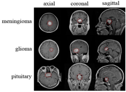
The tumor classification is based on statistics, intensity, symmetry, texture, etc., that use the tumor’s grey value. In the processing of the image, the extraction of the feature is a special type of dimensional reduction. However, the grey values of MRI tend to be modified because of an increase or in the presence of noise. When the data entered into an algorithm is too large to process and is presumed notoriously redundant, the data entered is transformed into a reduced representation set of features. The types of brain tumor is indicated in Figure 1.
Figure 1. Tumor types
The process of translating data into a set of functions is referred to as feature extraction. When the retrieved features are carefully picked, they will be extracted from the input data to extract relevant information in order to do the required task using this smaller representation rather than the full size input. In order to accurately characterize a large number of datasets, extracting features requires a reduction in the amount of resources required. One of the most difficult obstacles in interpreting complicated data is the quantity of variables involved. A huge number of variables needs a lot of memory and processing capacity, as well as a classification technique that matches the sample but isn't very generalizable to new ones. Feature extraction is a wide phrase that describes how variables are constructed to address these challenges while still effectively representing data.
The process of selecting a subset of relevant characteristics for generating powerful learning models by eliminating the most uninformative features from the data. Selection of features helps enhance model performance by eliminating the most uninformative features from the data.
• Effects of the dimensionality reduction.
• Speed up learning processes to enhance the capacity for generalization.
• Improvement of model performance.
The selection of features also helps people gain a better understanding of their data and tells them which features are important and how they relate to each other. In this method, we obtain a combination process for reduction of features by a Double-Weighted Feature Extraction Labelling Model with Priority Weighted Feature Selection. In other words, all own values are kept in a matrix. The first step in processing is the transformation without dimension limitation. Then numbers of own values are calculated that have the highest and most effective values. The proposed model assigns double weighted labelling for all extracted features by considering the edges and borders and then for most relevant features, priority is assigned for the weights that play a major role in tumor cell detection.
The main task of pathologists is the tissue observation and identification of specific histological attributes linked to the degree of malignancy. In a second step, the histological results are interpreted and the tumor grade is decided. In most cases, pathologists do not know exactly how many attributes are taken into account; they can however classify the tumors almost instantly and are ignorant of their complexity.
A number of methods have been employed to segment and predict the degree and volume of brain tumors. In their work, Mehrotra et al. [1] proposed a Fluid Cognitive Map (FCM) to establish the value of the tumor grade [2]. The authors used the soft calculation process of fuzzy cognitive maps for the FCM classification model, to know how to achieve 91 percent and 94 percent diagnostic accuracy of low and high grade brain tumors respectively. They proposed only the technique to characterize and accurately determine grades.
Demirhan et al. [3] suggested a technique which uses fusion to represent pictures better for the recognition of the face by extracting attributes through a Deep Convolution Neural Network (DCNN). They used Principal Component Analysis (PCA) to reduce the fused attribute's capacity. For two classes, the SVM machine classification is implemented. This technique shows that faces with serious occlusion and significant differences in confusion and scale can be distinguished. In conclusion, this technique reaches a reminder rate of 86 percent and an average precision of 94 percent.
Shantta and Basir [4] proposed a CNN recognition process which can acknowledge people based on face-to-face illustrations. The model first uses CNN to extract the attributes of the facet and then fuses the abstract characteristics [5] with the hue characteristics [6]. The grouping results can be obtained using the Soft-Max classifier [7]. They say that the proposed method in this study can achieve an accuracy of 66%. Deng [8] introduced a procedure in the use of a classical algorithms and CNN for abstracting brain tumors of the 2-D MRI brain. The empirical investigation took place on a real time set of cancer dimensions [9], locations, patterns and various pictorial strengths. In the classical algorithm, six traditional classification machines [10] were applied, especially the Support Vector Machine. The closest neighbors. Applied CNN with Keras and TensorFlow, then, because it produces better than regular performances. CNN achieved 94 percent accuracy.
Lu et al. [11] research describes the common practices used in extracting attributes in the first place and then extends the process of Deep Learning (DL) repeatedly utilized in the attribute extracted from section. They conclude that they relate to other approaches to machine learning. DL can differ from almost unprocessed primary information complex interactions of attributes and lower level attributes.
Huan et al. [12] suggested a technique based on Deep Neural Networks to completely automatize the classification of brain tumors. In the glioblastoma disease images in different degrees the intended algorithm was used. There is a new structure offered by a convolutionary network. Flowing planning is available in which the output of a core convolutionary network is not used for the following convergence network as an additional basis of data.
The feature extraction techniques used by Hossain et al. [13] used histograms of oriented grade rates, features from the discrete cosine transform domain and attributes extracted [14] from the CNN pre-trained models. In this model, "feature extraction for image selection using machine learning [15]," they concluded that the content classification attributes [16] removed from CNN produced best results.
Basheera and Ram [17] proposed a new way to classify benign and three different types of brain tumors using CNN. The tumor is mainly divided into a segmented ICA composite model from the MRI imagery. Deep attributes are extracted and arranged after the segmented image. The results were confirmed in a data set free of charge with the Harvard Medical School by measuring the results of the classification system.
Bhandari et al. [18] completed several trials that differ learning from start to finish and display that preferred tuning function presents a short collection of about one thousand skin damage images. The workouts are nevertheless minor rules which are able to achieve any typical outcome tasks. To examine the role of CNN in the brain tumor segment, the author first looks at CNN and conducted dissertations on the finding of a segmentation instance pipeline [19]. Also, look for a new field – radionics – to look for the future efficiency of CNNs. The quantitative characteristics of brain tumors [20], such as form, texture and signal intensity, are explored to predict clinical outcomes, such as existence and treatment reaction.
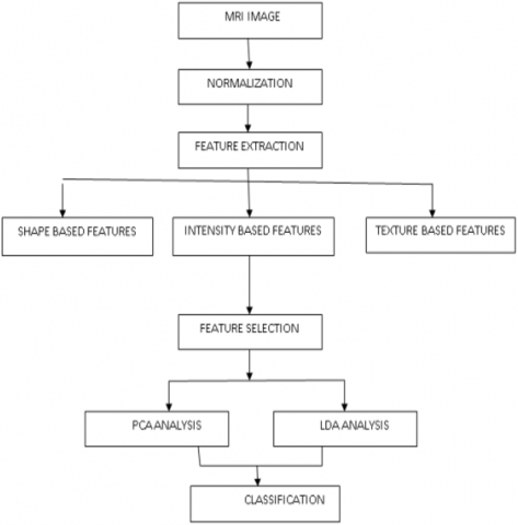
The feature extraction is the way to transform the data entry into a series of functions. It is the main step in developing any model classification and the aim of extracting relevant information that portrays each class. This proposed model extracts the relevant features from objects to form vector features. The classifiers then use these feature vectors to perceive a data unit with the objective rendering unit. Furthermore, for many datasets, large-scale feature selection is more critical. Dataset may contain more locally relevant and redundant features. Some existing Evolutionary Calculation (EC) schemes can therefore be used, but for a small feature selection, they are better. In addition, the high-performance feature selections with large solution sizes deliver low performance. This paper proposed a Double-Weighted Feature Extraction Labelling Model with Priority Weighted Feature Selection model for effective tumour cell detection. The framework of the proposed model is represented in Figure 2.
Figure 2. Proposed model framework
When carefully selected, the features represent the characteristics of the objects of interest to be offered for a complete lesion characterisation. Methods for extracting information from photos and objects are called extractions. A feature's class can be determined by looking at the feature's attributes. Extracting features or qualities that identify patterns from one another is the goal of feature extraction. The feature extracted should offer the input classifier type's features based on the image attributes described by vectors. Using this model's findings, we can extrapolate the following features. They actually are There is a lot of variation in shade and square variation when it comes to the circularity, irregularity, and area of a piece of art.
The structural information on intensity, form, and texture can be gleaned from the characteristics. Although these qualities are redundant, the goal of this stage is to discover their true potential. Redundancy can be reduced further by using function selection to eliminate redundant processes.
To investigate algorithms in depth, a subset of data functions is selected using the feature selection procedure. The most accurate subset is the one with the smallest number of dimensions. Variables are introduced one at a time to start, and the procedure continues until no additional addition significantly reduces error before stopping.
The problem of low-dimensional feature representation is avoided in this model. The data matrix n to N, which contains each ri as a image I vector in the combination with the MRI image dataset {I1, I2, I3, ……. IN} is represented.
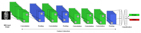
The Convolutionary Neural Network (CNN)s are components of an appropriate classification of the neural network technology. CNN has also exceeded many traditional, hand-crafted methods, and has the ability to automatically learn image representations. A CNN, each of which has an equal number of filters that are down-sample layers, and the completely connected layers that serve as classifiers, depends on one another locally connected convolutional layers. The suggested CNN for the detection of brain tumors using MRI images is illustrated in Figure 3. Three notions of the architecture of convolutionary neural networks are effective: receptive fields locally, weight sharing, and down-sampling. The local receiving field shows that each neuron is able to recognize a small section of the preceding layer with a convolution filter of the same size of 3 X 3.
Figure 3. Proposed CNN architecture
Further, in convolutional and down sampling layers’ local receptive fields are used. The convolutionary weight-sharing layer regulates and decreases the ability of the paradigm. Finally, it is done to reduce the spatial size of the image and to decrease free paradigm parameters. These concepts help CNN in recognition tasks to be strong and efficient. The image I is considered from the image dataset and the convolution representation is performed as
$I_{i, j}^{M}=f\left(\sum i \in D S\left(I_{M}\right)+x_{j}^{l-1} * y_{i}^{l}+T h\right)$ (1)
where, I is the image considered, M is the count of set of images considered, x,y are the image coordinates and Th is the threshold value for convolution representation. After representing the image in convolution form, the edges of the image are identified as
$E_{M}\left(I\left[l_{x}, l_{y}\right]\right)=\sqrt{\sum_{l=\mathrm{i}}^{\mathrm{M}}\left(I(x, y)-l_{m-1}\left(I\left[l_{x-1}, l_{y-1}\right]\right)\right)^{2} \times f_{M}^{I\left[l_{x}, l_{y}\right]}}+{x_{j}^{l-1}} * y_{i}^{l}$ (2)
The edges E are identified for extracting pixels with the region of an image I for tumor prediction is performed. The pixels within the range of edges are only considered and all the pixels are extracted as
PixelExtractor $\left(P E_{I}\right)=\sum_{x=1}^{M} \sum_{y=1}^{x} E_{i j}^{m} \| x_{j}-y_{i}||^{2}+\mathrm{x} * \mathrm{y}+f_{M}^{I\left[l_{x}, l_{y}\right]}$ (3)
To address the imbalanced class problem more directly, the suggested model employs a class structured cross-entropy loss function. For tumour prediction, all network layer variables as nL are evaluated, and the target function of the pixel extractor is computed as
$\operatorname{TargetF}(P E)=\sum_{I \in D S} \sum_{i<M} E_{M}^{l}+P E(I)+\lambda$ (4)
where, λ determines the relative value of tumour pixels. The pixels extracted are labelled as
$L(I(x, y))=\sum_{i} E_{M}+\lambda_{x . y}(P E)+\sum_{i} \sum_{j} \operatorname{TargetF}\left(I_{M}(x, y)\right)+L V$ (5)
where, LV is the labeling vector that is assigned to all the pixels extracted from the image I with the edges E. After labelling is performed, the loss levels of each pixel is considered. PEi values that are proportional to the number of samples in the I class can be chosen inversely for data loss for each layer that is calculated as
$I_{\text {loss }}(x, y$, Target $F)=\sum_{i}^{M} W_{i} L_{i} \log S_{n}-\sum_{i}^{M}\left(1-\mathrm{n} L_{i}\right)+\Delta E(i)$ (6)
where, Li is the loss level, $\Delta E$ is the change in the edge pixels extracted. After calculating the loss levels of every pixel, Double labelling is performed as
$D L(I(x, y))=L(I(x, y))+\sum_{i+1} E_{M}+\lambda_{x . y}(P E)+\min (L(i))+$ Th (7)
After double labelling is performed, the pixel contrast and intensity values are extracted for accurate tumour region identification. Histogram equalization model is used for intensity extraction and the quality improvement. The process is performed as
while (i < 255) do
if (HE1(i) <$\lambda$)
HE2(i) = 0
HE2(i+1) $\leftarrow$ HE1(i) + HE1(i+1)-HE2(i)
HE2(i+1) $\leftarrow$ HE1(i) + HE1(i+1)- HE2(i)
Else
HE2(i) $\leftarrow$ HE1(i)
End if
i $\leftarrow$ i + 1
end while
Based on the values identified, the final pixel labelling PL is performed as
$P L=\left\{\begin{array}{lr}0, & \text { if } \operatorname{pix}(I(i, j)=255 \text { or } 0 \\ 1, & \text { otherwise }\end{array}\right.$ (8)
The pooling layer is discussed, which conducts a down-sampling operation to reduce the spatial dimension of the coevolutionary layer. To begin, measure and then apply to the pooling mask and pooling type at the pooling layer. The pooling procedure is performed at the pixel values recorded by the pooling mask and multiplied by an applied coefficient. The process of pooling is performed as
$I(x, y)_{M}^{i}=f\left(D L_{i}^{i} p o o l\left(I_{M i}^{l}\right)+P E_{j}^{l}(M)\right)$ (9)
The priority weights are allocated based on the pixel values that contains tumor cells. The priority weights are allocated as
$W_{i, j}=\exp \left(\frac{\left.-\left(I_{i n}(x)-\mathrm{I}_{i n}(y)\right)^{2}+\max (P L(I(x, y)))\right)}{\left(\frac{\lambda^{2}}{2}\right) * \mathrm{PL}}\right)$
$+\frac{\lambda+\left(H E_{1}+H E_{2}\right)_{\text {avg }}+\max \left(\sum_{P L(i)}(i=0, \lambda=1)\right)}{\max \left(\sum_{E m} .\right) * T h}$ (10)
The tumor identification is performed based on the priority weights allocated based on the labelling of pixels. The tumor cells are identified and the prediction set is maintained as
TumorI $^{\mathrm{M}}(x, y)=D S^{(i)}(x, y)$
$+\frac{1}{W_{i, j}} \sum_{i=1}^{M} W_{i, j_{M}}^{-1}\left(\left(\left(x_{k}-y_{k}^{(i)}\right)-\min \left(I_{\text {loss }}(x, y\right.\right.\right.$, TargetF$\left.\left.)\right)\right)$
$+\max \left(\right.$ pixelExtractor $\left.\left.\left(P E_{I}\right)\right)\right)$ (11)
The calculation of Peak Signal to Noise Ratio is performed as
$M S E=\frac{\sum_{i=1}^{M} \mathrm{PE} \sum_{j=i}^{M} \mathrm{~W}(\mathrm{DL}(x, y)-\operatorname{Tumor} I(x, y))^{2}}{x * y}$ (12)
The absolute mean square error is calculated as the difference between the input and output means.
$A M S E=\frac{1}{W_{i, j}} \sum_{i=1}^{T} W_{i, j}|x-y|$ (13)
The error rate is measured as
Mean Square Error Rate
$(E r)=\frac{1}{x_{1} x_{2}} \frac{\sum_{i=1}^{M_{1}} \sum_{j=i}^{M_{2}}(\hat{f}(x, y)-f(x, y))^{2}}{\sum_{i=1}^{M_{1}} \sum_{j=i}^{M}(f(x, y))^{2}}$ (14)
The suggested work aims to investigate the automatic recognition of a brain tumour by merging convolutional neural networks with deep learning in order to achieve tumour identification automatically. The proposed model is written in Python and run in ANACONDA. The MRI image dataset is available in the link https://www.kaggle.com/navoneel/brain-mri-images-for-brain-tumor-detection. Brain tumour detection is a challenging and sensitive task that requires the classifier's skill. This paper describes the use of a Convolutional Neural Network (CNN) system to classify the type of brain tumour. Tumours can be identified by extracting relevant features from MRI images and utilising CNN with deep learning techniques. CNN can both save time and improve the identification of brain tumours. The proposed Double-Weighted Feature Extraction Labelling Model with Priority Weighted Feature Selection (DWLM-PWFS) model is compared to traditional Deep Convolutional Long Short-Term Memory (C-LSTM) method, and the findings reveal that proposed model is effective in detecting cancers. The proposed model is compared with the traditional methods in terms of Feature Extraction Accuracy, Feature Labelling Accuracy, Priority Allocation Time Levels, Feature Extraction Time, True Positive Rate and Tumour Detection Accuracy. The Table 1 represents the values of the grades of tumour and the suggested treatment.
The efficiency or precision of classifier is analyzed based on the error rate for each texture analysis method. The following terms true and false positive and true and false negative can describe this error rate.
True Positive (TP): In the presence of clinical abnormality the test results are positive.
True Negative (TN): In the absence of clinical abnormality the test result is negative.
False Positive (FP): In the absence of clinical abnormalities the test results are positive.
False Negative (FN): In the event of clinical abnormality, the test result is negative.
- sensitivity = recall = tp / t = tp / (tp + fn)
- specificity = tn / n = tn / (tn + fp)
- precision = tp / p = tp / (tp + fp)
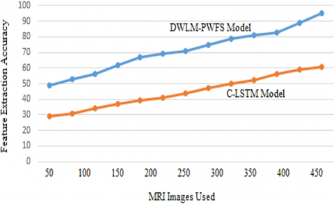
Feature extraction is a dimensionality reduction procedure that reduces an initial collection of raw data to more meaningful units for processing. The enormous number of variables in such large data sets necessitates a large number of computational resources to process. Feature extraction refers to approaches that choose and/or combine variables to form features, hence minimising the quantity of data which must be processed while properly and thoroughly characterizing the actual data set. The feature extraction accuracy of the proposed and traditional methods is represented in Figure 4.
Table 1. Tumor grades and models used
|
S.No |
Brain Tumor Classes |
Number of features |
Accuracy |
|
1 |
Low grade Gliomas, Metastatic |
100 features from GLCM |
72% |
|
2 |
Metastates, Gliomas |
4 features from histograms |
93% |
|
3 |
Low grade Gliomas, Metastatic, Metastatic, Normal Regions |
218 intensity and texture features |
85% |
|
4 |
Low grade Gliomas, Metastatic, Metastatic, Normal Regions, Normal Brain |
371 intensity features |
92% |
Figure 4. Feature extraction accuracy
Figure 5. Feature labelling accuracy
Data labelling is the act of recognising raw data and applying one or more relevant and informative labels to provide meaning so that a deep learning model can learn from it. Labels, for example, could determine whether or not an image contains a tumour, which words were spoken in an audio recording, or whether an x-ray reveals a tumour. Many applications, such as computer vision, natural language processing, and speech recognition, require data labelling. The feature labelling accuracy of the proposed and existing model is shown in Figure 5. The proposed modelling feature labelling accuracy is high that indicate the performance levels of the model.
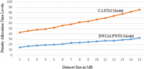
The priority allocation is performed to accurately identify the tumor cells by considering the most relevant features. The priority allocation time levels of the proposed and existing models ate clearly indicated in the Figure 6.
Figure 6. Priority allocation time levels
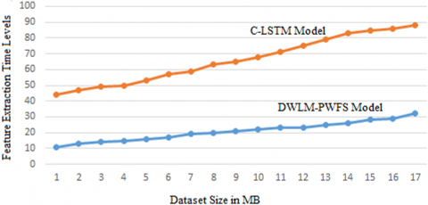
In deep learning, pattern recognition, and image processing, feature extraction starts with a set of measured data and builds derived values called features that are intended to be informative and non-redundant, facilitating subsequent learning and generalisation steps and, in some cases, leading to better human interpretations. Dimensionality reduction is related to feature; it can be translated into a smaller set of characteristics, also known as a feature vector. The process of determining a subset of the original features is referred to as feature selection. The features chosen are intended to contain the necessary information from the input data, allowing the task to be completed using this reduced representation rather than the entire initial data. The feature extraction time levels of the proposed and traditional method are indicated in Figure 7.
The performance of the tumor detection system depends on the accuracy levels achieved. The accuracy levels of the proposed and existing method are represented in Figure 8.
Figure 7. Feature extraction time
Figure 8. Tumour detection accuracy
Table 2. Algorithm evaluation in terms of accuracy and F1 score
|
Classifier |
DWLM-PWFS |
C-LSTM |
KNN |
SVM |
|
Accuracy % |
87 |
86 |
88 |
89 |
|
True Positive Rate |
0.92 |
0.91 |
0.93 |
0.94 |
The Table 2 indicates the accuracy and true positive rate of the proposed and existing models. The values indicate that the proposed model accuracy is better than the traditional methods.
Because of the varied nature of tumor cells, brain tumor classification is a difficult issue for radiologists. Recently, computer-aided diagnosis-based methods have claimed to diagnose brain tumors using magnetic resonance imaging as an assistive technology). In recent implementations of pre-trained models, characteristics are typically taken from bottom layers that differ between natural and medical images. This paper proposed a Double-Weighted Feature Extraction Labelling Model with Priority Weighted Feature Selection method for accurate tumour identification. In addition, the brain tumor detection task was performed using the CNN algorithm. In medical images such as magnetic resonance imaging, the CNN is precisely suitable for selecting an automated feature. In the proposed model, initially all the features are extracted and double labelling is performed using deep learning model with features taken from MRI image. Then, to classify the brain tumor, these features were reduced and most relevant features are considered by performing priority allocation to the weights allotted previously. The proposed model efficiently identifies the tumor for proper diagnosis. In future, we will research and use sophisticated strategies for pre-trained models with a large number of layers, and we will also be able to classify brain tumor using score based modelling with data enhancement techniques. We will also study the whole process based on sophisticated and score based characteristics retrieved from deep learning models with increased number of hidden layers.
[1] Mehrotra, R., Ansari, M.A., Agrawal, R., Anand, R.S. (2020). A transfer learning approach for AI-based classification of brain tumors. Machine Learning with Applications, 2: 100003. https://doi.org/10.1016/j.mlwa.2020.100003
[2] Mathew, A.R., Anto, P.B. (2017). Tumor detection and classification of MRI brain image using wavelet transform and SVM. 2017 International Conference on Signal Processing and Communication (ICSPC), Coimbatore, India, pp. 75-78. https://doi.org/10.1109/CSPC.2017.8305810
[3] Demirhan, A., Törü, M., Güler, I. (2014). Segmentation of tumor and edema along with healthy tissues of brain using wavelets and neural networks. IEEE Journal of Biomedical and Health Informatics, 19(4): 1451-1458. https://doi.org/10.1109/JBHI.2014.2360515
[4] Shantta, K., Basir, O. (2020). Brain tumor diagnosis support system: A decision fusion framework. IRA International Journal of Applied Sciences, 15(3): 30-47. http://dx.doi.org/10.21013/jas.v15.n3.p1
[5] Wang, H., Raj, B. (2017). On the origin of deep learning. arXiv preprint arXiv:1702.07800
[6] Sze, V., Chen, Y.H., Yang, T.J., Emer, J.S. (2017). Efficient processing of deep neural networks: A tutorial and survey. Proceedings of the IEEE, 105(12): 2295-2329. https://doi.org/10.1109/JPROC.2017.2761740
[7] Emmert-Streib, F., Yang, Z., Feng, H., Tripathi, S., Dehmer, M. (2020). An introductory review of deep learning for prediction models with big data. Frontiers in Artificial Intelligence, 3(4): 33733124. https://doi.org/10.3389/frai.2020.00004
[8] Deng, L. (2018). Artificial intelligence in the rising wave of deep learning: The historical path and future outlook [perspectives]. IEEE Signal Processing Magazine, 35(1): 180-177. https://doi.org/10.1109/MSP.2017.2762725
[9] Strogatz, S. (2018). One giant step for a chess-playing machine. New York Times.
[10] Farooq, M., Sazonov, E. (2017). Feature extraction using deep learning for food type recognition. International Conference on bioinformatics and biomedical engineering, Granada, Spain, pp. 464-472. https://doi.org/10.1007/978-3-319-56148-6_41
[11] Lu, X., Duan, X., Mao, X., Li, Y., Zhang, X. (2017). Feature extraction and fusion using deep convolutional neural networks for face detection. Mathematical Problems in Engineering, 2017: 1376726. https://doi.org/10.1155/2017/1376726
[12] Huan, E.Y., Wen, G.H., Zhang, S.J., Li, D.Y., Hu, Y., Chang, T.Y., Wang, Q., Huang, B.L. (2017). Deep convolutional neural networks for classifying body constitution based on face image. Computational and Mathematical Methods in Medicine, 2017: 9846707. https://doi.org/10.1155/2017/9846707
[13] Hossain, T., Shishir, F.S., Ashraf, M., Al Nasim, M.A., Shah, F.M. (2019). Brain tumor detection using convolutional neural network. 2019 1st International Conference on Advances in Science, Engineering and Robotics Technology (ICASERT), Dhaka, Bangladesh, pp. 1-6. https://doi.org/10.1109/ICASERT.2019.8934561
[14] Liang, H., Sun, X., Sun, Y., Gao, Y. (2017). Text feature extraction based on deep learning: A review. EURASIP Journal on Wireless Communications and Networking, 2017(1): 1-12. https://doi.org/10.1186/s13638-017-0993-1
[15] Havaei, M., Davy, A., Warde-Farley, D., Biard, A., Courville, A., Bengio, Y., Pal, C., Jodoin, P.M., Larochelle, H. (2017). Brain tumor segmentation with deep neural networks. Medical Image Analysis, 35: 18-31. https://doi.org/10.1016/j.media.2016.05.004
[16] Pereira, S., Pinto, A., Alves, V., Silva, C.A. (2016). Brain tumor segmentation using convolutional neural networks in MRI images. IEEE Transactions on Medical Imaging, 35(5): 1240-1251. https://doi.org/10.1109/TMI.2016.2538465
[17] Basheera, S., Ram, M.S.S. (2019). Classification of brain tumors using deep features extracted using CNN. Journal of Physics: Conference Series, 1172(1): 012016. https://doi.org/10.1088/1742-6596/1172/1/012016
[18] Bhandari, A., Koppen, J., Agzarian, M. (2020). Convolutional neural networks for brain tumour segmentation. Insights into Imaging, 11(1): 1-9. https://doi.org/10.1186/s13244-020-00869-4
[19] Seetha, J., Raja, S.S. (2018). Brain tumor classification using convolutional neural networks. Biomedical & Pharmacology Journal, 11(3): 1457. https://doi.org/10.13005/bpj/1511
[20] Ma, X., Dai, Z., He, Z., Ma, J., Wang, Y., Wang, Y. (2017). Learning traffic as images: a deep convolutional neural network for large-scale transportation network speed prediction. Sensors, 17(4): 818. https://doi.org/10.3390/s17040818