Hongyu Sun* | Yuerui Qi | Wenlei Tian | Geng Chen | Yana Wang
© 2021 IIETA. This article is published by IIETA and is licensed under the CC BY 4.0 license (http://creativecommons.org/licenses/by/4.0/).
OPEN ACCESS
This paper mainly analyzes the typical geological structure of the coal seam with scouring zone, and examines the channel features of the coal seam. Firstly, a detailed analysis was conducted on the propagation features of channel wave in complex coal seam with geological anomalies. Based on COMSOL Multiphysics, a three-dimensional (3D) medium geometry model was established for complex coal seam with scouring zone. Relying on the model, channel wave propagation was simulated by finite-element method, and the propagation features were analyzed thoroughly. The Ricker wavelet with a central frequency of 200Hz was employed to emulate the explosive source, and the excited vibration signal was measured along the coal seam. Experimental results show that the longer the propagation distance of the channel wave signal in the coal seam, the more stretched the channel wave train, and the later the arrival of the maximum envelope of the wave train. The maximum envelope of the wave train appeared earlier in the model with the scouring zone than in the model without the scouring zone. After the channel wave passed through the scouring zone, the maximum envelope of the wave train appeared later in the model with the scouring zone than in the model without the scouring zone.
channel wave signal propagation, scouring zone, finite-element method
In recent years, the mechanization of coal mining has accelerated coal mine exploration. Many countries with complex geological conditions, namely, China, are witnessing a quick depletion of the reserves of shallow coal resources. As coal mining gets deeper into the ground, the conditions of the coal seam become poorer. For example, deep coal seams often contain complex small structures and other geological anomalies. These complex factors destroy the continuity of the coal seam, destabilize the surrounding rock of the roadway, and deters the mechanized coal mining. What is worse, the geological anomalies might form a water channel or a gas storage site, which brings the hazards of water inrush and gas outburst on the top and bottom of the coal seam. If these anomalies are not detected timely, the work safety of coal mining will be at stake, and accidents might occur, endangering life and property safety [1].
Channel wave signal offers a promising tool for geophysical prospecting [2]. It is known for the good coupling with formation medium, high energy efficiency, long transmission distance, and high accuracy. The tool has been widely applied in coal detection, and laid the basis for formation detection in other fields [3]. Many scholars have explored the propagation features of channel wave in actual formations, especially the dispersion features. However, few have tackled the influence of small structures, e.g., scouring zone, on the propagation features of the wave [4]. The propagation features of elastic waves are usually analyzed by the elastic wave equation and geological methods [5-7].
This paper integrates the relevant methods and seismic exploration techniques in modern communication, and regards the coal seam as a channel. From the perspective of filtering [8, 9], the authors analyzed the influence of typical geological small structures in the coal seam on elastic wave propagation, and abstracted the channel features of the scouring zone for building a three-dimensional (3D) simulation model. The research results provide a theoretical guide for channel wave detection in complex coal seams. The contributions of this research are as follows:
(1) The analysis on the changing features of channel wave propagation in complex coal seams with scouring zone provides numerical references for coal mine detection, seismic exploration, oil exploration, and hydrological engineering. The relevant results help to capture the distribution and changes of stress fields in the coal seam, guide the work safety of coal mines, e.g., preventing water inrush, and provide analytical data for earthquake prediction. (2) The channel wave propagation model for typical geological small structures in coal seams is helpful for the smooth progress of geological exploration, and complements the shortcomings of ordinary ground penetrating radar (GPR).
2.1 Formation mechanism
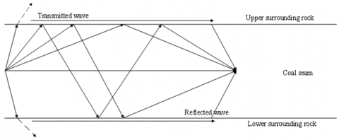
The coal seam is composed of sedimentary rocks and coal. The typical sedimentary rocks include sandstone, siltstone, mudstone, shale, and limestone. Since the coal seam differs greatly from the surrounding rock in physical properties, an elastic wave propagates faster in the upper and lower surrounding rocks than in the coal seam. As a result, the space between the upper and lower surrounding rocks becomes a strong wave impedance interface (Figure 1) [10].
Therefore, the coal seam can be regarded as a typical low-speed interlayer, comparable to a beam wave guide [11]. Once a longitudinal/transverse wave is excited in the coal seam, part of the excited energy undergoes repeated total reflections in the said interface as the wave propagates through the coal seam [12]. The reflected waves are imprisoned in the coal and surrounding rocks, and superimposed on each other, forming a set of interferences with strong energy points. The superimposed wave carries the features of channel wave.
Figure 1. Principle of channel wave formation
The above analysis shows that the channel wave is a seismic wave bound in the coal seam, which has a long propagation distance, a high energy, a strong dispersion, and an easy-to-identify waveform [13]. During the formation of the channel wave, the relative size of wave velocity and coal seam/surrounding rock density is more important than the absolute values.
2.2 Channel wave signal classification
By vibration direction, channel waves can be divided into love-type channel wave (L wave) and Rayleigh-type channel wave (R wave) [14-17].
(1) L wave
Figure 2. Sketch map of L wave
L wave is formed as shear horizontal (SH) waves propagate along the x direction and interfere with each other in the coal seam. The particles of the L wave vibrate parallel to the coal seam (y direction) and perpendicular to the propagation direction of the seismic wave. According to the propagation path of the SH wave in the coal seam, the ray method can be adopted to derive the dispersion equation of the L wave (Figure 2). The wavefront FB of the SH wave propagates downward from point A on the coal seam, and the plane wavefront FBE passes through the BCE path, and is reflected at point E. When superimposed, the incident angle of seismic waves is θ.
To ensure the existence of the plane harmonic, the constructive interference needs to meet the following condition:
$\omega (\overset{\to }{\mathop{BCE}}\,/{{v}_{s2}}-4\varphi )=2n\pi$ (1)
where, BCE is the distance from point B through point C to point E; 4φ is the phase shift in one-time total reflection from the coal seam to the surrounding rock.
By the principle of total reflection, we have:
$\tan \varphi \text{=}\frac{{{\mu }_{1}}\sqrt{1-C_{L}^{2}v_{s1}^{2}}}{{{u}_{2}}\sqrt{C_{L}^{2}/v_{s2}^{2}-1}}$ (2)
Then:
$\begin{align} & \overrightarrow{BCE}=2\text{d}\cos \theta \\ & \cos \theta =C_{L}^{2}/v_{s2}^{2}-1 \\\end{align}$ (3)
Thus, the dispersion equation can be expressed as:
$\begin{align} & \frac{\pi {{f}_{N}}}{{{C}_{LN}}}\sqrt{C_{LN}^{2}-1} \\ & ={{\tan }^{-1}}\left[ {{\rho }_{N}}v_{SN}^{2}\frac{\sqrt{1-C_{LN}^{2}v_{SN}^{2}}}{\sqrt{c_{LN}^{2}-1}} \right]+n\pi \\\end{align}$
$n=0,1,2......$ (4)
where, $v_{S N}=v_{S 1} / v_{S 2} ; \rho_{N}=\rho_{1} / \rho_{2} ; f_{N}=2 f d / v_{s 2} ; C_{L N}=C_{L} / v_{s 2}$.
(2) R wave
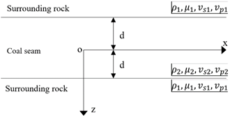
The R wave is formed by the interference of the compressional (P) wave and the shear vertical (SV) wave in the coal seam. The particles of the R wave vibrate in the direction synthesized by two directions: the z direction perpendicular to the coal seam, and the direction parallel to the seismic wave. In the propagation direction, the seismic wave formed by P-SV interference perturbates elliptically. Figure 3 is the Rayleigh channel wave symmetry 3-layer model , where ρ1,Vp1, Vs1, and μ1 are the density, longitudinal wave velocity, shear wave velocity, and shear modulus of the surrounding rock, respectively; ρ2, Vp2, VS2, and μ2 are the density, longitudinal wave velocity, shear wave velocity, and shear modulus of the coal seam, respectively; 2d is the thickness of the coal seam. Similar to the derivation of the L wave, the dispersion equation of the R wave, i.e., the periodic equation in the normalized three-layer symmetric model, can be established as:
$\begin{align} & C\tan \left[ \frac{\pi {{f}_{N}}}{{{C}_{RN}}}\sqrt{C_{RN}^{2}-1}-n\pi \right] \\ & \tan \left[ \frac{\pi {{f}_{N}}}{{{C}_{RN}}}\sqrt{\frac{{{C}_{RN}}}{{{v}_{P2N}}}{{}^{2}}\text{-}1}\text{-n}\pi \right] \\ & \text{+}D\tan \left[ \frac{\pi {{f}_{N}}}{{{C}_{RN}}}\sqrt{C_{RN}^{2}-1}-n\pi \right] \\ & +A\tan \left[ \frac{\pi {{f}_{N}}}{{{C}_{RN}}}\sqrt{{{(\frac{{{C}_{RN}}}{{{v}_{P2N}}})}^{2}}-1}-n\pi \right]+B=0 \\\end{align}$ $n=0,1,2.......$ (5)
Figure 3. Rayleigh channel wave symmetry 3-layer model
3.1 Parameters and source term
The scouring zone appears as the coal seam is eroded by rivers or glaciers. In most cases, the zone is filled by sandy deposits. Scouring is the most common non-geological cause that makes the coal seam abnormal. The scouring zone is either syngenetic or metagenetic, depending on the stage of formation.
Syngenetic scouring zone, also known as intralayer scouring zone, is formed before the sandy deposition and coal accumulation. Due to repeated seawater erosion, the roof of the coal seam and the bottom of the overlying limestone are uneven, creating a “toad roof”. The size and depth of the scouring zone are relatively small, because scouring takes place before the coal seam is covered by the overlying sediment.
Table 1. Parameters of the coal seam with scouring zone
|
Parameters |
υp (m/s) |
υs (m/s) |
ρ (kg/m3) |
|
Surrounding rock |
3,710 |
1,990 |
2,600 |
|
Coal seam |
2,200 |
1,100 |
1,390 |
|
Scouring zone |
2,200 |
1,100 |
2,800 |
Metagenetic scouring zone is formed after the coal seam is covered by sediments. The scouring takes place during the deposition or after the formation of the coal seam. Near the scouring zone, the coal is darker, with a high ash content. The size and depth of this scouring zone are relatively large. Hence, metagenetic scouring zone seriously damages the coal seam, adding difficulty to geological exploration and coal mining.
Table 1 presents the parameters of the coal seam with scouring zone.
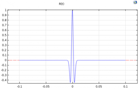
The numerical simulation of elastic waves requires a source term. With simple shape, short duration, and fast convergence, the Ricker wavelet is a suitable tool for numerical simulations [18]. In the time domain, the Ricker wavelet can be expressed as:
$R(\text{t})\text{=}\left[ 1\text{-}2{{\pi }^{2}}\text{f}_{M}^{2}{{(t-{{t}_{0}})}^{2}} \right]\exp \left[ -{{\pi }^{2}}f_{M}^{2}{{(t-{{t}_{0}})}^{2}} \right]$ (6)
where, fm is the main frequency; t0 is the initial moment.
Figure 4 shows the Ricker wavelet at the main frequency of 200Hz.
Figure 4. Ricker wavelet at 200Hz
The Ricker wavelet can achieve the momentary excitation energy of the explosive source, at the duration of 0.0055 and amplitude of 10^8. Therefore, this wavelet was selected as the source term of our simulation.
3.2 3D equivalent medium geometric model of scouring zone
To analyze channel wave propagation in the scouring zone, the first step is to model the geometry of that zone. Compared with intact formations, the coal seam containing the scouring zone is generally thin or missing. The scouring zone can be characterized by a wide long-lasting stripe on the plane. For convenience, it is assumed that the scouring zone is similar to a flat ellipsoid, and that the upper and lower surrounding rocks and the residual coal seam are isotropic media.
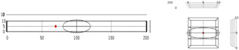
Suppose no water is accumulated in the scouring zone. There are sandy deposits with uniform density in the zone. Figure 5 presents the 3D equivalent medium geometric model of the scouring zone.
The 3D model is a three-layer medium model with a length of 200m, a width of 10m, and a height of 10m. The upper and lower surrounding rocks are 4m thick and the coal seam is 2m thick. Located in the coal seam, the scouring zone is centered at x=100m, with a radius of 20m in x direction, a radius of 5m in y direction, and a radius of 1m in z direction. The source is a 200Hz Ricker wavelet. Figure 6 provides the top view and side view of the model.
Figure 5. 3D equivalent medium geometric model of scouring zone (right denotes inside of model)
Figure 6. Top and side views of the coal seam with scouring zone
Figure 7. Coal seam model without scouring zone
Without changing any parameter, the geometric model of the coal seam without scouring zone was established (Figure 7).
4.1 Channel wave propagation in the scouring zone
In theory, the scouring zone can be approximated by a uniform tubular geometric model with different cross-sectional areas. This paper analyzes an infinitely small cube in the scouring zone (Figure 8). The side length and side area of the cube are denoted as Δx and Δs, respectively. In addition, the velocity, the velocity added with an increment, the pressure, and the pressure added with an increment are denoted as v, v+Δv, P, and p+Δp, respectively. According to Newton’s Second Law of Motion, the resultant force of the small cube can be expressed as:
$F=ma$ (7)
After analyzing the force of the small cube, F can be described as:
$F=(P+\Delta P)\cdot \Delta S\text{-}P\cdot \Delta S\text{=}\Delta S\cdot \Delta P$ (8)
Combining formulas 7 and 8:
$\Delta S\cdot \Delta P\text{=ma=m}\frac{\partial v}{\partial t}=\rho \cdot \Delta S\cdot \Delta x\cdot \frac{\partial v}{\partial t}$ (9)
It is known that:
$\Delta P=\rho \cdot \Delta x\cdot \frac{\partial v}{\partial x}$ (10)
Let Δx→0. Then,
$\frac{\partial P(x,t)}{\partial x}=\rho (x,t)\cdot \frac{\partial v(x,t)}{\partial t}$ (11)
It can be inferred that:
$\frac{\partial P(x,t)}{\partial t}=\rho (x,t)\cdot \frac{\partial v(x,t)}{\partial x}$ (12)
Figure 8. Small cube
Let A be the cross-sectional area; ρx(x,t) be the linear density in x direction. Then, the relationship between linear density and volume density can be expressed as: ρx (x,t)=ρ(x,t)⋅A.
Therefore, formulas 10 and 11 can be respectively rewritten as:
$\frac{\partial P(x,t)}{\partial x}=\frac{{{\rho }_{x}}(x,t)}{A}\cdot \frac{\partial v(x,t)}{\partial t}$ (13)
$\frac{\partial P(x,t)}{\partial x}=\frac{A}{{{\rho }_{x}}(x,t)}\cdot \frac{\partial P(x,t)}{\partial t}$ (14)
If ρx(x,t) changes very little with x and t, ρx(x,t) can be regarded as a constant. Then, the partial derivative of x on both sides of formula 12 can be obtained:
$\frac{{{\partial }^{2}}P(x,t)}{\partial {{x}^{2}}}=\frac{{{\rho }_{x}}(x,t)}{A}\cdot \frac{{{\partial }^{2}}v(x,t)}{\partial t\cdot \partial x}$ (15)
The partial derivative of t can be obtained from formula (13):
$\frac{{{\partial }^{2}}v(x,t)}{\partial x\cdot \partial t}=\frac{A}{{{\rho }_{x}}(x,t)}\cdot \frac{{{\partial }^{2}}P(x,t)}{\partial {{t}^{2}}}$ (16)
From formulas 14 and 15, we have:
$\frac{{{\partial }^{2}}P(x,t)}{\partial {{x}^{2}}}=\frac{{{\partial }^{2}}P(x,t)}{\partial {{t}^{2}}}$ (17)
Form formulas 12 and 13, the partial derivative of t can be obtained as:
$\frac{{{\partial }^{2}}v(x,t)}{\partial x\cdot \partial t}=\frac{{{\rho }_{x}}(x,t)}{A}\cdot \frac{{{\partial }^{2}}v(x,t)}{\partial {{t}^{2}}}$ (18)
$\frac{{{\partial }^{2}}v(x,t)}{\partial {{x}^{2}}}=\frac{A}{{{\rho }_{x}}(x,t)}\cdot \frac{{{\partial }^{2}}P(x,t)}{\partial t\cdot \partial x}$ (19)
From formulas 17 and 18, we have:
$\frac{{{\partial }^{2}}v(x,t)}{\partial {{x}^{2}}}=\frac{{{\partial }^{2}}v(x,t)}{\partial {{t}^{2}}}$ (20)
Formulas 17 and 20 can be solved by separation of variables. Substituting v(x,t)=f(x)⋅g(t) into formula 20, we have:
$\frac{f\prime\prime (x)}{f(x)}=\frac{g\prime\prime (t)}{g(t)}$
Suppose $\frac{f^{\prime \prime}(x)}{f(x)}=k_{1}^{2}$ and $\frac{g^{\prime \prime}(x)}{g(x)}=k_{2}^{2}$. Then, the following formulas can be derived:
$f(x)={{e}^{\pm {{k}_{1}}x}}={{e}^{\pm {{k}_{2}}x/\eta }}$
$g(t)={{e}^{\pm {{k}_{2}}x}}$
Therefore, the solution to formula 19 can be expressed as:
$v(x,t)={{v}^{+}}(t-x)-{{v}^{-}}(t+x)$ (21)
$\begin{align} & P(x,t)={{P}^{+}}(t-x)-{{P}^{-}}(t+x) \\ & =\frac{\rho \eta }{A}\left[ {{V}^{+}}(t-x)+{{v}^{-}}(t+x) \right] \\\end{align}$ (22)
Figure 9. Adjacent cubes in the scouring zone
Then, it is assumed that the scouring zone contains N small cubes with a short length h, and different cross-sectional areas. Figure 9 shows two adjacent cubes, namely, cube k-1 and cube k.
The pressure P and velocity v remain constant across the contact between cube k-1 and cube k:
$\begin{align} & {{v}_{k-1}}(h,t)={{v}_{k}}(0,t) \\ & {{p}_{k-1}}(h,t)={{p}_{k}}(0,t) \\\end{align}$ (23)
where, k-1=1,2,3...N-1. Substituting formulas 20 and 21 to formula 22, we have:
$\begin{align} & v_{k-1}^{+}(t-h)-v_{k-1}^{+}(t+h)=v_{k-1}^{+}-v_{k-1}^{-} \\ & \frac{\rho \eta }{{{A}_{k-1}}}\left[ v_{k-1}^{+}(t-h)+v_{k-1}^{+}(t+h) \right] \\ & =\frac{\rho \eta }{{{A}_{k}}}\left[ v_{k-1}^{+}+v_{k-1}^{-} \right] \\\end{align}$ (24)
Solving formula 24, we have:
$v_{k-1}^{+}(t-h)=\frac{1}{2}\left[\begin{array}{c}\frac{A_{k}+A_{k-1}}{A_{k}} \cdot v_{k}^{+}(t) \\ +\frac{A_{k-1}-A_{k}}{A_{k}} \cdot v_{k}^{-}(t)\end{array}\right]$$=\frac{A_{K}+A_{K-1}}{2 A_{k}}\left[v_{k}^{+}(t)-\frac{A_{k}-A_{k-1}}{A_{k}+A_{k-1}} \cdot v_{k}^{-}(t)\right]$ (25)
$v_{k-1}^{-}(t+h)=\frac{1}{2}\left[\begin{array}{c}\frac{A_{k-1}-A_{k}}{A_{k}} \cdot v_{k}^{+}(t) \\ +\frac{A_{k-1}+A_{k}}{A_{k}} \cdot v_{k}^{-}(t)\end{array}\right]$$=\frac{A_{k}+A_{k-1}}{2 A_{k}}\left[-\frac{A_{k}-A_{k-1}}{A_{k}+A_{k-1}} \cdot v_{k}^{-}(t)+v_{k}^{+}(t)\right]$ (26)
Substituting $K_{k-1}=\frac{A_{k}-A_{k-1}}{A_{k}+A_{k-1}}$ into formulas 25 and 26, we have:
$K_{k-1}^{+}(t-h)=\frac{1}{1+{{K}_{k-1}}}\left[ v_{k}^{+}(t)-{{K}_{k-1}}v_{k}^{-}(t) \right]$ (27)
$K_{k-1}^{-}(t+h)=\frac{1}{1+{{K}_{k-1}}}\left[ -{{K}_{k-1}}v_{k}^{+}(t)-v_{k}^{-}(t) \right]$ (28)
Applying Laplace transform on formulas 26 and 27, we have:
$\begin{align} & K_{k-1}^{+}(s)\cdot {{e}^{-sh}}=\frac{1}{1+{{K}_{k-1}}}\cdot \left[ v_{k}^{+}(s)-{{K}_{k-1}}v_{k}^{-}(s) \right] \\ & K_{k-1}^{-}(s)\cdot {{e}^{-sh}}=\frac{1}{1+{{K}_{k-1}}}\cdot \left[ {{K}_{k-1}}v_{k}^{+}(s)-v_{k}^{-}(s) \right] \\\end{align}$ (29)
Then, the velocity of cube k-1 can be obtained as:
$\begin{align} & {{V}_{k-1}}(s)=\frac{{{e}^{sh}}}{1+{{K}_{k-1}}} \\ & \cdot \left[ \begin{matrix} 1 & -{{K}_{k-1}} \\ -{{K}_{k-1}}{{e}^{-2sh}} & {{e}^{-2sh}} \\\end{matrix} \right]\cdot \left[ \begin{matrix} V_{k}^{+}(s) \\ V_{k}^{-}(s) \\\end{matrix} \right] \\\end{align}$ (30)
To study the channel wave at the transmitter and receiver, formulas 12 and 13 were compared with formula 29. Then, the channel wave propagation in the scouring zone can be described in the form of an equivalent circuit:
$\begin{align} & \frac{\partial U}{\partial \text{x}}\text{=}L\frac{\partial I}{\partial \text{t}} \\ & \frac{\partial I}{\partial \text{t}}\text{=}L\frac{\partial U}{\partial \text{x}} \\\end{align}$ (31)
Let V0(s) be the channel wave velocity of the transmitter; Z0 be the wave impedance of the transmitter. Then, Vo(s) can be expressed as:
$V_{0}(s)=V_{1}(s)+\frac{P_{1}(\mathrm{~s})}{Z_{0}}$ (32)
Then, the wave impedance Zl of cube L can be expressed as:
${{Z}_{l}}=\frac{\rho }{{{A}_{L}}}$ (33)
Combining formulas 22 and 33, P(s) can be expressed as:
${{P}_{l}}(s)=Zl\cdot \left[ V_{l}^{+}(s)+V_{l}^{-}(s) \right]$ (34)
Substituting formula 33 into formula 31, we have:
$\begin{array}{*{35}{l}} {{V}_{0}}(s)=V_{1}^{+}(s)-V_{1}^{-}(s)+\frac{{{Z}_{1}}}{{{Z}_{0}}}\left[ V_{1}^{+}(s)+V_{1}^{-}(s) \right] \\ =\frac{{{Z}_{1}}+{{Z}_{0}}}{{{Z}_{0}}}V_{1}^{+}(s)+\frac{{{Z}_{1}}-{{Z}_{0}}}{{{Z}_{0}}}V_{1}^{-}(s) \\ =\left[ \frac{{{Z}_{1}}+{{Z}_{0}}}{{{Z}_{0}}}\frac{{{Z}_{1}}-{{Z}_{0}}}{{{Z}_{0}}} \right]\cdot \left[ \begin{matrix} V_{1}^{+}(s) \\ V_{1}^{-2}(s) \\\end{matrix} \right] \\ =\left[ \frac{{{Z}_{1}}+{{Z}_{0}}}{{{Z}_{0}}}\frac{{{Z}_{1}}-{{Z}_{0}}}{{{Z}_{0}}} \right]\cdot {{V}_{1}}(s) \\\end{array}$ (35)
The space beyond the receiver was regarded as an infinitely long isotropic homogeneous medium. No reflection will occur after the wave passes through the scouring zone, and spreads to the external surrounding rock. Thus, we have:
${{V}_{0}}(s)=\left[ \frac{2}{1+{{K}_{0}}}-\frac{2{{K}_{0}}}{1+{{K}_{0}}} \right]\cdot {{V}_{1}}(s)$ (36)
${{V}_{N+1}}(s)=\left[ \begin{matrix} V_{N+1}^{+}(s) \\ 0 \\\end{matrix} \right]=\left[ \begin{matrix} {{V}_{h}}(s) \\ 0 \\\end{matrix} \right]=\left[ \begin{array}{*{35}{l}} 1 \\ 0 \\\end{array} \right]\cdot {{V}_{h}}(s)$ (37)
Substituting formulas 30 and 37 into formula 36, we have:
$V_{0}(s)=\left[\frac{2}{1+K_{0}} \frac{-2 K_{0}}{1+K_{0}}\right]$$\cdot \frac{e^{N s h / 1}}{\prod_{k=1}^{N}\left(1+K_{k}\right)} \cdot\left[\begin{array}{cc}1 & K_{1} \\ -K_{1} e^{-2 s h} & e^{-2 s h}\end{array}\right] \cdot\left[\begin{array}{cc}1 & K_{2} \\ -K_{2} e^{-2 s h} & e^{-2 s h}\end{array}\right]$$\cdots\left[\begin{array}{cc}1 & K_{N} \\ -K_{N} e^{-2 s h} & e^{-2 s h}\end{array}\right] \cdot\left[\begin{array}{l}1 \\ 0\end{array}\right] \cdot V_{h}(s)$ (38)
Set the T for sampling to 2h. Then, Z-1=e-sT=e-2sh. Through the z transform, we have:
$V_{0}(Z)=\left[2 \frac{-2 K_{0}}{1+K_{0}}\right] \cdot \frac{Z^{-N / 2}}{\prod_{k=1}^{N}\left(1+K_{k}\right)}$$\cdot\left[\begin{array}{cc}1 & K_{1} \\ -K_{1} Z^{-1} & Z^{-1}\end{array}\right] \cdot\left[\begin{array}{cc}1 & K_{2} \\ -K_{2} Z^{-1} & Z^{-1}\end{array}\right]$$\cdots\left[\begin{array}{cc}1 & K_{N} \\ -K_{N} Z^{-1} & Z^{-1}\end{array}\right] \cdot\left[\begin{array}{c}1 \\ 0\end{array}\right] \cdot V_{h}(Z)$ (39)
Then, the transfer function can be obtained for the channel wave propagating through the scouring zone:
$H(Z)=\frac{V_{\mathrm{h}}(\mathrm{Z})}{V_{0}(Z)}=\frac{\prod_{k=1}^{N}\left(1+K_{k}\right)}{Z^{-N / 2} \cdot\left[\begin{array}{cc}\frac{2}{1+K_{0}} & \frac{-2 K_{0}}{1+K_{0}}\end{array}\right] \cdot \prod_{k=1}^{N}\left[\begin{array}{cc}1 & K_{N} \\ -K_{N} Z^{-1} & Z^{-1}\end{array}\right] \cdot\left[\begin{array}{c}1 \\ 0\end{array}\right]}$
$=\frac{\left(1+K_{0}\right) \cdot \prod_{k=1}^{N}\left(1+K_{k}\right)}{Z^{-N / 2} \cdot\left[\begin{array}{cc}2 & -2 K_{0}\end{array}\right] \cdot \prod_{k=1}^{N}\left[\begin{array}{cc}1 & K_{N} \\ -K_{N} Z^{-1} & Z^{-1}\end{array}\right] \cdot\left[\begin{array}{l}1 \\ 0\end{array}\right]}$ (40)
4.2 Model verification
COMSOL Multiphysics can solve partial differential equations or sets of such equations, and simulate real physical phenomena by finite-element method. The calculation range covers various physical fields, ranging from heat conduction to structural mechanics. COMSOL Multiphysics simulation could offer mathematical solutions to real-world physical phenomena.
Figure 10. Verification of wave guide phenomenon
This subsection verifies the reasonability of our theoretically deduced model for the coal seam with the scouring zone, i.e., the presence of wave guide phenomenon of the coal seam. This phenomenon is a prerequisite for the formation of channel waves. During the verification, measuring points were arranged with an interval of 1m from the source to 150m down in the vertical direction to the coal seam. The vibration amplitude captured in the verification process is shown in Figure 10, where the x axis is the propagation time, and the y axis is the vibration amplitude; from top to bottom, the layers are the upper surrounding rock, the coal-rock interface, the coal seam, and the lower surrounding rock [19]. It can be inferred that the energy of the channel wave is mainly distributed in the coal seam, which extends from the coal-rock interface to the upper and lower surrounding rocks. The energy in the surrounding rock was almost zero. Hence, the wave guide phenomenon of the coal seam was fully verified.
4.3 Channel wave propagation features in the scouring zone
Taking the Ricker wavelet with a main frequency of 200Hz as the seismic source (coordinates: 1.5, 5), the channel wave propagation was simulated in the coal seam without the scouring zone. The measuring points were deployed at 10, 40, 70, 100, 130 and 160 in the x direction. The captured data were imported to MATLAB to plot the waveform of the channel wave (Figure 11). Then, the channel waveform in the coal seam without the scouring zone was compared with that in the coal seam with the scouring zone (Figure 12). In the two figures, the x axis is the measuring points, and the y axis is the propagation time.
Figure 11. Channel waveform in the coal seam without the scouring zone
Figure 12. Channel waveform in the coal seam with the scouring zone
Judging by the received signal of the channel wave excited by the unstructured Ricker wavelet (Figure 11), the maximum amplitude of the propagating channel wave in the coal seam without the scouring zone dropped from -5^10-4 to 5^10-4 at x=10m to -5^10-5 to 5^10-5 at x=160m, that is, the amplitude decayed to one tenth of the original. Meanwhile, the vibration wave train was continuously elongated, and the vibration time of particles at x=10m tended to 0 after 0.02s. With the propagation of the channel wave, however, the vibration wave train stretched to x=160m; the vibration time extended from 0.06s to 0.12s; reflected waves of small amplitude appeared. In the coal seam with the scouring zone (Figure 12), the propagation of the channel wave brought more obvious amplitude decline. The maximum amplitude at x=160m was less than 2^10-8, i.e., the amplitude decayed to one tenth of the original. But the vibration wave train was not significantly elongated.
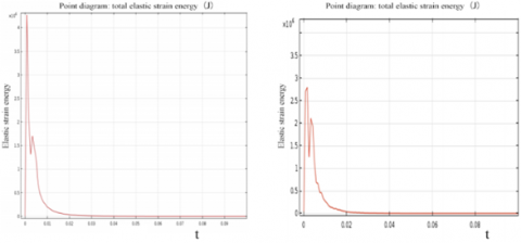
From the two figures, it can be learned that, the longer the propagation distance of the channel wave in the coal seam, the more stretched the channel wave train, and the later the arrival of the maximum envelope of the wave train. When the channel wave reaches the scouring zone, the signal will appear as a standing wave disturbance at the edge of the zone, owing to the medium difference between the zone and the coal seam, and the reflection of the surrounding rock. As a result, the maximum envelope of the wave train in the coal seam with the scouring zone appears earlier than that in the coal seam without the scouring zone. After the wave passes through the zone, the presence of the scouring zone reduces the propagation distance, and increases the number of reflections of the channel wave. Therefore, the maximum envelope of the wave train in the coal seam with the scouring zone appeared much earlier than that in the coal seam without the scouring zone. During the propagation of the channel wave, the large initial explosive force will deform the coal seam and the surrounding rock to a certain extent. During the deformation, the work done by external forces is converted into energy stored in the solid. Figure 13 presents the change of elastic strain energy in the two models.
Figure 13. Variation in total elastic strain energy in the coal seam with the scouring zone (left) and the coal seam without the scouring zone (right)
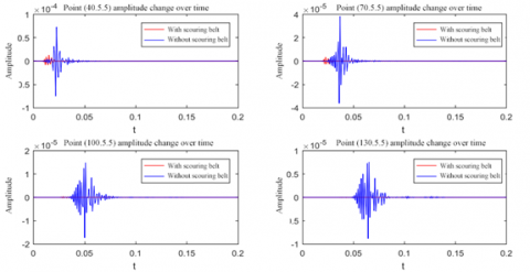
Figure 14. Amplitude changes at four points
The two models exhibited similar trends in total elastic strain energy. In both models, the energy first increased rapidly and then plunged since 0.01s. Under the influence of the reflected wave energy, the energy slightly rebounded, and finally ended to zero in 0.02s. The difference is that the total elastic strain energy in the model without the scouring zone was greater than that in the model with that zone. The latter model had more obvious reflected waves, which is consistent with the previous discussion. Figure 14 compares the amplitude changes at two points (40, 5, 5), (70, 5, 5) before the scouring zone, and two points after that zone (100, 5, 5), (130, 5, 5).
With the elapse of time, the amplitude at the four points reached the peak in sequence, and the number of peaks continued to decrease. This means the scouring zone has a great impact on amplitude fluctuation. The overall amplitude of the model with the scouring zone was much smaller than that of the model without the zone, whether the channel wave was before or after that zone. Figure 15 shows the amplitude-frequency relationship at the four points.
Figure 15. Amplitude-frequency relationship at four points
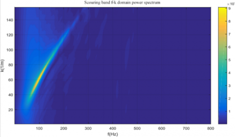
Figure 16. Power spectrum of the scouring zone in the f-k domain
As shown in Figure 15, the scouring zone has a major impact on channel wave propagation at every model. In the model without the scouring zone, the amplitude of the channel wave changed significantly, and a small peak appeared at 300Hz to 400Hz. The amplitude was zero before 300Hz, and the frequency did not reach the minimum frequency of vibration. As the channel wave propagated, the amplitude started to increase at 300Hz, and peaked at 500Hz to 600Hz with a smaller height. The scouring zone is located at x=80m to x=120m. In the model with the scouring zone, the amplitude increased slowly with the frequency before the wave reached the scouring zone, peaking at 400Hz. After the wave passed through the zone, the amplitude basically did not change with the increasing frequency. It can be learned that the scouring zone absorbs lots of wave energy, and almost blocks the propagation of the channel wave. Only a very small amount of channel wave energy can bypass the scouring zone to arrive at the receiver.
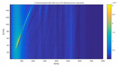
The channel wave signal should be located accurately, in order to determine the location and shape of anomalous geological structures through channel wave exploration. However, it is no easy task to find the signal blocking position, due to the complexity of unground wave field, severe noise interference, and the dispersion features of the channel wave. To solve the problem, the channel wave signal was converted to the f-k domain, and the noise and other interfering components were filtered, in the light of the dispersion features of the channel wave. Figures 16-17 show the power spectra of the scouring zone and the channel wave in the f-k domain, respectively.
Figure 17. Power spectrum of the channel wave in the f-k domain
As shown in Figures 16 and 17, the energy of the Ricker wavelet mainly concentrated near the main frequency in the early stage of excitation. As the seismic wave propagated in the coal seam, the wave train was gradually elongated, and the energy peak shifted from low frequency to high frequency, accompanied with a large attenuation. Compared with the model with the scouring zone, the model without the scouring zone saw high energy dispersion and obvious wave lengthening. In the model with the scouring zone, the channel wave energy fell in 0-300Hz; in the other model, the energy was observed even beyond 500Hz. This means the scouring zone concentrates the energy to the main frequency band, and prevents the movement to high frequencies.
(1) There are various small structure in actual coal seams. Different small structures have vastly different effects on channel wave propagation in the coal seam.
(2) The longer the propagation distance of the channel wave signal in the coal seam, the more stretched the channel wave train, and the later the arrival of the maximum envelope of the wave train. The maximum envelope of the wave train appeared earlier in the model with the scouring zone than in the model without the scouring zone. After the channel wave passed through the scouring zone, the maximum envelope of the wave train appeared later in the model with the scouring zone than in the model without the scouring zone.
(3) The total elastic strain energy in the model without the scouring zone was greater, with a taller peak, than that in the model with that zone. The overall amplitude of the model with the scouring zone was much smaller than that of the model without the zone, whether the channel wave was before or after that zone. The power spectra in the f-k domain show that the scouring zone concentrates the energy to the main frequency band, and prevents the movement to high frequencies.
This work was supported by Shandong Provincial Natural Science Foundation under Grant No. ZR2020MF014.
[1] Guo, Y.J., Yang, L., Song, S.Q. (2019). Analysis of Channel Wave Propagation Characteristics in Coal Seam. Coal Technology, 38(10): 61-63.
[2] Jiao, Y., Wei, J.S., Yang, X.L. (2019). Channel wave detection technology and application of collapsed column in coal mine. China Energy and Environmental Protection, 41(1): 62-69.
[3] Yi, X.L. (2017). Analysis Of Elastic Wave Propagation Characteristics of Typical Small Geological Structure in Coal Measure Strata. Shandong University of Science and Technology, 3.
[4] Evison, F.F. (1955). A coal seam as a guide for seismic energy. Nature, 176(4495): 1224-1225. https://doi.org/10.1038/1761224a0
[5] Riedel, C., Musayev, K., Baitsch, M., Hackl, K. (2021). Seismic exploration in tunneling using full waveform inversion with a frequency domain model. PAMM, 20(1): e202000141. https://doi.org/10.1002/pamm.202000141
[6] He, W., Ji, G., Dong, S., Li, G. (2017). Theoretical basis and application of vertical Z-component in-seam wave exploration. Journal of Applied Geophysics, 138: 91-101. https://doi.org/10.1016/j.jappgeo.2017.01.008
[7] Wang, B., Liu, S., Zhou, F., Hu, Z., Huang, L., Jiang, Y. (2016). Dispersion characteristics of SH transmitted channel waves and comparative study of dispersion analysis methods. Journal of Computational and Theoretical Nanoscience, 13(2): 1468-1474. https://doi.org/10.1166/jctn.2016.5069
[8] Zhang, L., Xu, L., Wei, Z., Feng, C. (2021). Study on in-seam wave response characteristics of reflection in fault bearing coal seam of Shuangliu Coal Mine. Geotechnical and Geological Engineering, pp. 1-10. https://doi.org/10.1007/s10706-021-01908-7
[9] Teng, J., Li, S., Jia, M., Lian, J., Liu, H., Liu, G., Zhang, W. (2020). Research and application of in‐seam seismic survey technology for disaster‐causing potential geology anomalous body in coal seam. Acta Geologica Sinica‐English Edition, 94(1): 10-26. https://doi.org/10.1111/1755-6724.14372
[10] Greenfield, R.J., Wu, S.T. (1991). Electromagnetic wave propagation in disrupted coal seams. Geophysics, 56(10): 1571-1577. https://doi.org/10.1190/1.1442967
[11] Hu, Z.A., Zhang, P., Xu, G. (2018). Dispersion features of transmitted channel waves and inversion of coal seam thickness. Acta Geophysica, 66(5): 1001-1009. https://doi.org/10.1007/s11600-018-0192-4
[12] Li, X., Wang, J., Guo, X. (2021). Analysis and practice of detection methods for goafs in complex coal mines. In Journal of Physics: Conference Series, 2006(1): 012056. https://10.1088/1742-6596/2006/1/012056
[13] Buchanan, D.J., Davis, R., Jackson, P.J., Taylor, P.M. (1981). Fault location by channel wave seismology in United Kingdom coal seams. Geophysics, 46(7): 994-1002. https://doi.org/10.1190/1.1441248
[14] Yang, Z., Ge, M.C., Wang, S.G. (2009). Characteristics of transmitting channel wave in a coal seam. Mining Science and Technology (China), 19(3): 331-336. https://doi.org/10.1016/S1674-5264(09)60062-4
[15] Kaur, B., Singh, B. (2021). Rayleigh-type surface wave in nonlocal isotropic diffusive materials. Acta Mechanica, 232: 3407–3416. https://doi.org/10.1007/s00707-021-03016-2
[16] Ji, G.Z., Zhang, P.S., Guo, L.Q., Yang, S.T., Ding, R.W. (2020). Characteristics of dispersion curves for Love channel waves in transversely isotropic media. Applied Geophysics, 17(2): 243-252. https://doi.org/10.1007/s11770-019-0798-6
[17] Guo, Y., Zhang, J., Ju, Y., Guo, X. (2019). A theoretical investigation of channel wave multipath propagation in a coal seam. Mathematical Problems in Engineering, 2019: 4314582. https://doi.org/10.1155/2019/4314582
[18] Buchanan, D.J. (1986). The scattering of SH‐channel waves by a fault in a coal seam. Geophysical prospecting, 34(3): 343-365. https://doi.org/10.1111/j.1365-2478.1986.tb00471.x
[19] Greenhalgh, S.A., Zhou, B., Pant, D.R., Green, A. (2007). Numerical study of seismic scattering and waveguide excitation in faulted coal seams. Geophysical Prospecting, 55(2): 185-198. https://doi.org/10.1111/j.1365-2478.2007.00604.x